• The Vertical Structure of Warm Ionised Gas in the Milky Way

  B. M. Gaensler,^A,D G. J. Madsen,^A,B, S. Chatterjee^A and S. A. Mao^{C A}Institute of Astronomy, School of Physics, The University of Sydney, NSW 2006, Australia
  ^BDepartment of Astronomy, University of Wisconsin, Madison WI 53706, USA
  ^CHarvard-Smithsonian Center for Astrophysics, Cambridge MA 02138, USA
  ^DARC Federation Fellow; email: bgaensler@usyd.edu.au

  Abstract: We present a new joint analysis of pulsar dispersion measures and diffuse H$\alpha$ emission in the Milky Way, which we use to derive the density, pressure and filling factor of the thick disk component of the warm ionised medium (WIM) as a function of height above the Galactic disk. By excluding sightlines at low Galactic latitude that are contaminated by H ii regions and spiral arms, we find that the exponential scale-height of free electrons in the diffuse WIM is $1830^{+120}_{-250}$ pc, a factor of two larger than has been derived in previous studies. The corresponding inconsistent scale heights for dispersion measure and emission measure imply that the vertical profiles of mass and pressure in the WIM are decoupled, and that the filling factor of WIM clouds is a geometric response to the competing environmental influences of thermal and non-thermal processes. Extrapolating the properties of the thick-disk WIM to mid-plane, we infer a volume-averaged electron density $0.014\pm 0.001$ cm^-3, produced by clouds of typical electron density $0.34\pm 0.06$ cm^-3 with a volume filling factor $0.04\pm 0.01$. As one moves off the plane, the filling factor increases to a maximum of $\sim 30\%$ at a height of $\approx$1–1.5 kpc, before then declining to accommodate the increasing presence of hot, coronal gas. Since models for the WIM with a $\approx 1$ kpc scale-height have been widely used to estimate distances to radio pulsars, our revised parameters suggest that the distances to many high-latitude pulsars have been substantially underestimated.

  Keywords: galaxies: ISM — Galaxy: halo, structure — globular clusters: general — ISM: structure — pulsars: general

1 Introduction

The interstellar medium (ISM) of the Milky Way is a complex, multi-phase environment. Much of the ISM is an ionised gas at temperatures of $10^{4}-10^{6}$ K, requiring one or more vast sources of ongoing energy injection. In the modern picture of the ISM (see Ferrière 2001, for a review), ionised gas consists of two main phases: a hot “coronal” component at temperatures of $\sim 10^{5}-10^{6}$ K, and a warm ionised medium (WIM) of temperature $\sim 10^{4}$ K.

The WIM is most easily identified in H$\alpha$ and other optical recombination lines, which show that much of this gas corresponds to H ii regions around massive stars. However, most H ii regions are seen only at low Galactic latitudes. Further from the plane, pulsar dispersion measures (DMs), free-free absorption of low-frequency Galactic synchrotron emission, interstellar scattering of compact radio sources, and faint H$\alpha$ and H$\beta$ emission all demonstrate the existence of a widespread, diffuse WIM, not associated with individual stars (see overviews by Kulkarni & Heiles 1987; Reynolds 1990a). In the rest of this paper, we use WIM to refer only to this diffuse component, disregarding individual H ii regions.

The diffuse WIM has a typical volume-averaged free electron density $n\approx 0.01-0.1$ cm^-3 and an electron temperature $T_{e}\approx 8000$ K (e.g., Reynolds 1990a; Weisberg et al. 2008). Scattering and dispersion of high-latitude pulsars demonstrate that the diffuse component of the WIM is distributed in a thick disk, extending more than a kpc above and below the Galactic plane with a roughly exponential fall-off in density (Readhead & Duffett-Smith 1975; Reynolds 1989; Nordgren et al. 1992). The power required to maintain the ionisation state of the thick-disk WIM is $\sim 5\times 10^{41}$ ergs s^-1, a vast rate of energy injection that can seemingly only be supplied by the photo-ionising flux of all the hot stars in the Galaxy (Reynolds et al. 1984, 1990b). Questions remain, however, over how these ultraviolet photons propagate to large distances above the Galactic plane (Reynolds 1990c; Miller & Cox 1993), and whether the spectrum of the photon field produced by massive stars is consistent with the observed line ratios in the WIM (Reynolds & Tufte 1995; Heiles et al. 1996a; Madsen et al. 2006). Many other edge-on spiral galaxies also have a faint, thick WIM disk, seen in deep H$\alpha$ observations (Rand 1998; Dettmar 2004). All these results make clear that the WIM is a key part of the feedback process between the stellar and gaseous components of a galaxy, and that it connects the energetics and dynamics of the disk and the halo. There is thus considerable motivation to understand the density, spatial distribution and extent of the WIM in the Milky Way and in other galaxies.

Our own Galaxy is unique in that the DMs of radio pulsars can provide the free-electron column of the WIM for thousands of lines of sight, allowing one to develop a smooth underlying model for the three-dimensional Galactic distribution of $n$ (e.g., Taylor & Cordes 1993; Gómez et al. 2001). Integrating such a distribution allows one to also predict the emission measure (EM) along any sightline. However, even when interstellar extinction is taken into account, the predicted EMs are vastly smaller than those inferred from diffuse H$\alpha$ emission, from low-frequency absorption in the spectra of non-thermal radio sources, or from free-free radio emission (e.g., Peterson & Webber 2002; Sun et al. 2008). Because DMs have a linear dependence on the free electron density while EMs depend on the square of the electron density, the inference is that even far from the plane, the WIM is not a smooth, homogeneous medium, but is clumped into discrete clouds or layers (Reynolds 1977, 1991b; Pynzar’ 1993). In the following sections, we review some recent attempts to model this structure.

1.1 Modeling The WIM

1.1.1 The NE2001 Model

Recognising the limitations of a smooth, homogeneous WIM, Cordes & Lazio (2002, 2003) developed a detailed model, termed “NE2001”, for the structure of ionised gas in the Galaxy. The NE2001 model consists of a thin disk of scale height 140 pc associated with low-latitude H ii regions; a thick-disk WIM layer as discussed above, with a scale height of 950 pc; large-scale structure associated with spiral arms; cavities and density enhancements corresponding to known features in the local ISM; and individual clumps and voids needed to model specific regions of enhanced/reduced scattering or dispersion. The NE2001 model can predict the DM, EM, angular broadening, scintillation bandwidth and other parameters for any sightline integrated to any distance. It is widely used to estimate distances to radio pulsars for which there is no other distance indicator other than their DMs.

The NE2001 model attempts to provide a comprehensive description of the WIM, and can be continually improved as more DMs and other data are obtained. However, as Cordes & Lazio (2002) acknowledge, the NE2001 model fails to correctly predict the DMs of some pulsars in high-latitude globular clusters. For example, the 22 pulsars in the globular cluster 47 Tuc have an average DM of 24.4 pc cm^-3 and are at a distance of $\approx 5$ kpc (Camilo et al. 2000; Gratton et al. 2003). Pulsars in this cluster are included as an input to the NE2001 model, but the prediction of NE2001 is DM $=42.1$ pc cm^-3, in significant disagreement with the observations. More broadly, Lorimer et al. (2006) have shown that if NE2001 is applied to the new pulsars subsequently discovered in the various surveys that used the Parkes multibeam receiver, the inferred vertical distribution of these sources in the Galaxy has a scale height about a factor of two lower than expected.

The NE2001 model also has other difficulties at high latitudes. At the north Galactic pole, NE2001 predicts EM $\approx 0.05$ pc cm^-6. This is more than order of magnitude smaller than that observed (Reynolds 1991b; Peterson & Webber 2002; Haffner et al. 2003), suggesting that there is substantial clumping of the WIM at large distances from the Galactic plane, not included in NE2001 (see also discussion by Reynolds 1991b, 1997).

Meanwhile, Sun et al. (2008) have attempted to simultaneously reconcile extragalactic Faraday rotation measurements and all-sky maps of Galactic radio emission with the distribution of $n$ predicted by NE2001. They show that a joint fit to all these data requires an anomalously strong halo magnetic field, and an unrealistically low scale-height for Galactic cosmic rays. Sun et al. (2008) argue that if the scale-height of the thick-disk WIM in the NE2001 model were increased from 950 pc to $\sim 2$ kpc, a self-consistent model for the Galactic distribution of thermal gas, magnetic fields and cosmic rays could then be derived.

1.1.2 The BMM06 Model

The arguments in §1.1.1 suggest that the scale height and volume filling factor of the thick-disk WIM need to be re-evaluated. A detailed study of this issue has been carried by Berkhuijsen et al. (2006), hereafter BMM06, who used measurements of EM and DM for 157 pulsars to derive statistics on the density, scale height and filling factor of the WIM. BMM06 argued that both the internal cloud electron density, $N$ and volume filling factor, $f$, of the clumpy WIM evolve with a source’s vertical distance, $z$, above or below the Galactic plane. They fit the data with a model in which $N$ decays exponentially, while $f$ grows exponentially, with $z$. The expressions for their best fits are:

$$N(z)=N_{0}~{}e^{-\frac{z}{H_{N}}},~{}f(z)=f_{0}~{}e^{+\frac{z}{H_{f}}},$$ (1)

with scale heights

$$H_{N}=710_{-120}^{+180}~{}{\rm pc},~{}H_{f}=670_{-130}^{+200}~{}{\rm pc},$$ (2)

and extrapolated mid-plane values

$$N_{0}=0.41\pm 0.06~{}{\rm cm}^{-3},f_{0}=0.05\pm 0.01.$$ (3)

The resulting volume-averaged density of the thick-disk WIM, $n\equiv fN$, remains roughly constant at $n\approx 0.02$ cm^-3 up to $z\sim 1$ kpc, implying a much larger effective scale height for the WIM layer than had been assumed by all previous authors. At higher $z$, BMM06 argue that the filling factor takes on a constant value $f\stackrel{{\scriptstyle>}}{{{}_{\sim}}}0.3$, while $N$ continues to decay. As discussed by Sun et al. (2008), the NE2001 model cannot successfully predict the free-free emission seen at 23 GHz by the WMAP experiment, but incorporating the function $f(z)$ derived by BMM06 (see Eqn. [1] above) produces a good match to the data.

The BMM06 model clearly offers a number of improvements over previous work in its description of the WIM at high $z$. However, there are several important caveats and limitations associated with that study. First, for 95% of the pulsars used by BMM06, no independent estimates of distance (or hence of $z$) were available, so BMM06 used the distances predicted by the NE2001 model, and assumed errors of 20% in these distances. However, as we noted in §1.1.1, the NE2001 model can be in error by much more than this at high Galactic latitudes. Conversely, BMM06 explicitly excluded from their sample all pulsars in globular clusters or in the Magellanic Clouds, eliminating a substantial number of sources with reliable, independent distances.

A second limitation of BMM06 (and also of the subsequent study by Berkhuijsen & Müller 2008) is that their data sets consist of paired estimates of DM and EM for each pulsar. While the DM is a direct integral of $n$ from the observer to the source, the EMs are derived from H$\alpha$ data, which correspond to integrals to infinity, attenuated by dust extinction. BMM06 scaled down the EM values to account for the finite distance of each pulsar, but this calculation propagates the significant distance uncertainties in NE2001 into the EM values. Furthermore, scaling the EMs requires one to assume a WIM scale height, introducing a degeneracy into their subsequent fitting of the EMs to derive this same scale height. BMM06 corrected the EMs for extinction using standard reddening laws, but such corrections assume that dust and gas are well mixed along the line of sight. A inhomogeneous dust distribution, combined with significant distance uncertainties for most pulsars, can result in an erroneous extinction correction.

Finally, BMM06 considered pulsars with $60^{\circ}<\ell<360^{\circ}$ and $|b|>5^{\circ}$ (where $\ell$ and $b$ are Galactic longitude and latitude, respectively). As we will show in §3.1, the DMs of many pulsars at $|b|<40^{\circ}$ are contaminated by H ii regions and by other low-latitude structure. When trying to extract the properties of the WIM in the thick disk, the DMs and EMs of such pulsars will increase the scatter in the data and will reduce the signal-to-noise ratio of the underlying signal.

Overall, we conclude that while the approach of BMM06 provides several new insights into the behaviour of the WIM as a function of $z$, there are large systematic uncertainties that need to be incorporated into the parameters they extract from the data.

1.1.3 Scope Of This Paper

The discussion in §1.1.1 and §1.1.2 illustrates the strengths and weaknesses of the NE2001 and BMM06 models. Specifically, NE2001 is a detailed description of ionised gas along existing sightlines, but has limited predictive power at high $z$ where the number of existing sightlines is sparse. BMM06 provide a comprehensive joint analysis of EMs and DMs, and lay out a functional form for the $z$-dependence of the thick-disk WIM that is a significant improvement over that of NE2001. However, their analysis suffers from the significant uncertainties introduced by adopting distances from NE2001, and by trying to correct EMs for extinction and for the finite path length to the pulsars in their sample.

In this paper, we complement these previous studies, with a simple attempt to model the overall structure of the diffuse WIM. Our main thrust is to re-apply the analysis of Reynolds (1989), who plotted DM${}_{\perp}\equiv$ DM$.\sin|b|$ vs. $z$ for $\sim 35$ pulsars with known distances, and compared this to the predictions of simple geometric models. While this approach has been repeated in various subsequent papers (e.g., Nordgren et al. 1992; Gómez et al. 2001; Berkhuijsen & Müller 2008), the much larger sample of pulsars now available affords us the luxury of being able to filter the data to avoid contamination by the clumps, spiral arms and H ii regions incorporated in NE2001, and to thus boost any signal produced by the truly diffuse WIM. In §2, we review the sample of pulsars with known, reliable, distances and define our sample of 53 sightlines. In §3 we use a cut on these DMs in Galactic latitude to derive a substantially revised scale-height of the thick-disk WIM, and then combine these DMs with separate data on EMs (i.e., not matched to pulsar sightlines, as carried out by BMM06 and Berkhuijsen & Müller 2008) to confirm the contention of BMM06 that the data are most simply explained if the volume filling factor of this layer evolves with $z$. In §4 we discuss the implications of our calculations for the distances to pulsars, for the structure of the WIM, and for the transition from warm to million-degree gas in the Galactic halo.

2 Pulsars with Reliable Distance Estimates

Independent distances for pulsars can be determined through a variety of techniques. Most commonly, pulsar distances are derived kinematically, in which measurements are made of the systemic velocities of foreground clouds seen in H i absorption (either against emission from the pulsar itself or against an associated object such as a supernova remnant). A model for Galactic rotation can then be used to convert these velocities into upper and/or lower limits on the pulsar’s distance (see Frail & Weisberg 1990 for a review).

While the kinematic approach produces reliable distances for many pulsars, there is a key difficulty in using these data to study the properties of the thick-disk component of the WIM. Since our explicit aim is to study the diffuse component of the WIM, we wish to avoid lines of sight that pass through more complicated regions of the ISM. Since kinematic distances rely on the clumpy and complicated nature of interstellar gas to produce discrete absorption features, sightlines with good H i absorption measurements are precisely those we wish to exclude if we want to study a diffuse component of the ISM. We thus exclude kinematic distances from further consideration, and below focus on three remaining samples of pulsars with distances determined independently of the foreground ISM properties. In any case, even when using only these other distance indicators, we will argue in §3.1.2 that one must exclude lines of sight for which $|b|<40^{\circ}$ to avoid contamination by H ii regions and spiral structure. Since H i absorption distances are not feasible for pulsars with $|b|\stackrel{{\scriptstyle>}}{{{}_{\sim}}}10^{\circ}$ (see, e.g., Weisberg et al. 2008), this makes moot any concerns as whether H i absorption distances should be included in our sample.

2.1 Pulsars with Parallaxes

The most reliable pulsar distances come from parallaxes, derived either through interferometric measurements or through pulsar timing. The pulsar catalogue of Manchester et al. (2005) lists 34 such pulsars which are also radio emitters (and hence have DM measurements). From this sample, we then eliminate seven objects for which the uncertainty in the parallax is greater than 33%, and also discard the Vela pulsar (PSR B0833–45), because the DM of this nearby pulsar is dominated by contributions from its associated young supernova remnant (Backer 1974; Desai et al. 1992).

2.2 Pulsars in Globular Clusters

Our second reliable sample are radio pulsars in globular clusters. The on-line compilation of such sources maintained by Paulo Freire lists 137 pulsars in 25 globular clusters. The DMs of pulsars within each cluster show a small level of variation, resulting both from ionised gas internal to the cluster (Freire et al. 2001) and from small-scale angular fluctuations in the Galactic DM between adjacent sight lines (Shishov & Smirnova 2002; Ransom 2007). However, the fractional variation in DM for each cluster is very small: the largest scatter in DM is for NGC 6760, for which the fractional variation between the two detected pulsars is $\approx 2\%$. We correspondingly consider each globular cluster as a single datum (regardless of how many pulsars the cluster contains), and adopt the mean and standard deviation of the pulsar DMs in that cluster as the representative value and uncertainty of the DM, respectively, for that cluster. Distances to each cluster have been taken from the on-line version of the compilation of Harris (1996). The distances were derived from the colour-magnitude diagram of each cluster by identifying the mean magnitude of the horizontal branch population, and as an ensemble should be reliable to $\approx 15\%$ (C. Heinke, private communication); we consequently adopt this as the fractional distance uncertainty for each cluster.

2.3 Pulsars in the Magellanic Clouds

Our final sample are pulsars in the Magellanic Clouds. The pulsar catalogue of Manchester et al. (2005) lists 14 radio pulsars in the Large Magellanic Cloud (LMC) and five radio pulsars in the Small Magellanic Cloud (SMC) (see also Crawford et al. 2001; Manchester et al. 2006). Since the SMC and LMC themselves have significant DM contributions (Gaensler et al. 2005; Manchester et al. 2006; Mao et al. 2008), these systems can only provide an upper limit on the Galactic DM contribution along these sight lines. For the LMC, the lowest DM is that of PSR J0451–67, but there is uncertainty as to whether this pulsar is actually in the LMC, or is a Galactic foreground source (Manchester et al. 2006). We correspondingly adopt the next highest DM, 65.8 pc cm^-3 for PSR J0449–7031, as our upper limit in the direction of the LMC. For the SMC, the lowest DM is 70 pc cm^-3 for PSR J0045–7042. We assume distances to the LMC and SMC of 50 and 61 kpc, respectively (Walker 2003; Alves 2004, and references therein).

3 Analysis

3.1 The Distribution of Dispersion Measures

The DM of a pulsar is defined as

$${\rm DM}=\int_{0}^{d}n(l)~{}dl,$$ (4)

where $d$ is the distance to the pulsar and $n(l)$ is the free electron density along a line element $dl$. The distributions of DM${}_{\perp}\equiv$ DM$.\sin|b|$ as a function of $z$ for the 51 measurements (§2.1 & §2.2) and two upper limits (§2.3) are shown in Figure 1. It is immediately clear that for pulsars with vertical heights in the range $10\stackrel{{\scriptstyle<}}{{{}_{\sim}}}z\stackrel{{\scriptstyle<}}{{{}_{\sim}}}1000$ pc, the average value of DM_⟂ steadily increases with $z$, indicating that such sources sit within the Galactic electron layer. For heights $z\stackrel{{\scriptstyle>}}{{{}_{\sim}}}1000$ pc, values of DM_⟂ saturate at $\approx 25-30$ pc cm^-3, correspondingly demonstrating that the electron layer falls off in density at these values of $z$. This saturation value is consistent with the upper limits for the LMC and SMC. In this sense, the data clearly reproduce the findings of many previous studies (Reynolds 1989, 1991a; Savage et al. 1990; Bhattacharya & Verbunt 1991; Nordgren et al. 1992; Miller & Cox 1993; Gómez et al. 2001; Cordes & Lazio 2003; Hill et al. 2005; Berkhuijsen & Müller 2008, BMM06).

The overall distribution of ionised gas in the thick disk is reasonably described by a single plane-parallel layer (e.g., Haffner et al. 2003). To confirm that our data are consistent with such a geometry, and to estimate the scale height of this structure, we compare our measurements to a planar distribution of free electron density, $n(z)$, which falls off exponentially with increasing $z$:

$$n(z)=n_{0}~{}e^{-\frac{z}{H_{n}}},$$ (5)

where $n_{0}$ is the extrapolated density of ionised gas at mid-plane and $H_{n}$ is the corresponding scale height. Integrating Equation (5) out to a given distance then gives the predicted distribution of DM${}_{\perp}(z)$:

$${\rm DM}_{\perp}(z)=n_{0}~{}H_{n}~{}\left(1-e^{-\frac{z}{H_{n}}}\right).$$ (6)

3.1.1 Exponential Fit To All Data

We have fit the 51 measurements in Figure 1 to Equation (6) using a Levenberg-Marquardt algorithm (Press et al. 1992) (the two upper limits from the Magellanic Clouds are excluded from the fit, but are used as independent tests on the validity of any fitted model). Note that since the errors in DM_⟂ are negligible compared to the errors in $z$, we neglect the former and adopt DM_⟂ as our independent variable, with each datum weighted by the inverse square of the error in $z$.

A fit of all the data to Equation (6) does not converge. This is due to the very small errors in $z$ for pulsars with distances from parallaxes: since there is no single curve that passes through all these points, the resulting $\chi^{2}$ is always high, with no set of fit parameters that correspond to a significant minimum. This problem can be mitigated by recognising that although the errors in distances to individual pulsars are indeed small, there is an additional systematic effect, in that random clumps of electrons along individual sightlines cause each measurement to deviate from the smooth underlying model (Gómez et al. 2001; Cordes & Lazio 2002).

Rather than explicitly incorporate individual clumps toward each pulsar as for the NE2001 model, we represent the overall systematic limitations of the data by including in the fit an additional fractional uncertainty (added in quadrature) to the value of $z$ for each pulsar (see, e.g., Savage et al. 1990). Adding successively larger fractional errors establishes that an additional 10% systematic uncertainty allows the fit to Equation (6) to converge, with a reduced chi-squared, $\chi^{2}_{r}$, of 12.3 for 49 degrees of freedom. The best-fit parameters are $H_{n}=1010^{+40}_{-170}$ pc and $n_{0}=0.031^{+0.004}_{-0.002}$ cm^-3, where the uncertainties have been determined via a bootstrap algorithm (Efron & Tibshirani 1993), and correspond to the most compact 68% interval of bootstrap realisations around the best-fit values. The corresponding curve is plotted as a dashed line in Figure 1: this fit is consistent with the upper limits on DM_⟂ for the Magellanic Clouds, and is quite similar to the thick-disk component of NE2001, for which $H_{n}=950$ pc and $n_{0}=0.035$ cm^-3 (plotted as a dot-dashed line in Fig. 1).

3.1.2 Exponential Fit To High-Latitude Data Only

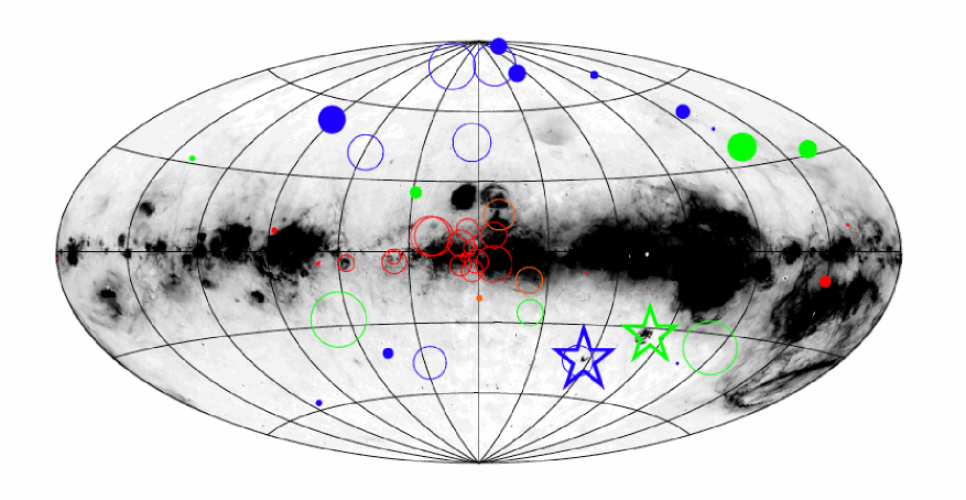
Figure 2: Aitoff projection in Galactic coordinates of pulsars with known, reliable, distances, super-imposed on the all-sky distribution of H$\alpha$ intensity (as derived by Finkbeiner 2003). The Galactic Centre is at the centre of the projection; colours and symbols are as in Figure 1. The centre of each symbol marks the coordinates of the corresponding source, while the diameter of each symbol is proportional to $\log_{10}({\rm DM}.\sin|b|)$ for that source. The greyscale is linear, ranging from 0 to 20 rayleighs.

While the results in §3.1.1 demonstrate that we can reproduce the findings of previous studies, the quality of the overall fit is reasonably poor. In particular, the best-fit curve substantially over-estimates DM_⟂ for most pulsars at $z>1000$ pc. A possible cause of this discrepancy is indicated in Figure 2, where we plot the distribution of our sample on the sky in Galactic coordinates. This demonstrates that there is a significant concentration of sources (mainly pulsars in globular clusters) in the Galactic plane and toward the Galactic Centre, for which the DMs are relatively high. This is simply understood as resulting from these pulsars being viewed not just through the thick-disk component of the WIM, but also through an additional thin-disk layer, corresponding to the dense, turbulent, ionised gas in individual H ii regions and supershells. The greyscale in Figure 2 clearly demonstrates this effect (see also Fig. 6 of BMM06), showing that low-latitude pulsars usually lie behind complicated regions of enhanced H$\alpha$ and EM.

We have correspondingly colour-coded the data in Figure 1 by Galactic latitude. It can indeed be seen that the red and orange points tend to lie above the blue and green ones, demonstrating that for a given $z$, sources at low $|b|$ tend to have higher values of DM_⟂ than at high $|b|$. To isolate the thick disk component, we thus fit to successive subsets of the data, selected by adopting a minimum threshold for $|b|$, $|b|_{\rm min}$, and thereby excluding sources contaminated by the thin-disk component of the WIM.

The results of these fits for $0^{\circ}\leq|b|_{\rm min}\leq 75^{\circ}$ are shown in Figure 3. This plot demonstrates that the quality of the fit is relatively poor, $\chi^{2}_{r}\approx 12-13$, for $0^{\circ}\leq|b|_{\rm min}\leq 30^{\circ}$, but is significantly improved, $\chi^{2}_{r}\approx 4-5$, for fits with $40^{\circ}\leq|b|_{\rm min}\leq 65^{\circ}$ (above this value, the sample size becomes too small to be meaningfully analysed). We adopt as our best description of ionised gas in the thick disk the lower latitude threshold that maximises the size of the sample while maintaining a good fit. This value is $|b|_{\rm min}=40^{\circ}$, for which $\chi^{2}_{r}=5.2$ (for 13 degrees of freedom); the corresponding 15 systems are indicated as blue data points in Figures 1 and 2. The fit to these data yields $H_{n}=1830^{+120}_{-250}$ pc and $n_{0}=0.014\pm 0.001$ cm^-3, shown by the solid line in Figure 1. The bootstrap approach incorporates the added uncertainties due to systematic deviations from the smooth underlying model. Thus although $\chi^{2}_{r}\gg 1$, the errors in $H_{n}$ and $n_{0}$ meaningfully characterise the confidence intervals on these parameters.

Our estimate of $H_{n}$ is substantially larger than that proposed by previous authors, as summarised in Table 1. However, our fit is clearly a good description of virtually all the high latitude data, especially those pulsars at high $z$. The implied integrated electron column density toward the Galactic poles is DM${}_{0}\equiv n_{0}H_{n}=25.97^{+0.02}_{-2.35}$ pc cm^-3, consistent with the upper limits from pulsars in the Magellanic Clouds, and comparable to the integrated vertical DM found in most previous studies.

The reason for our much larger estimate of $H_{n}$ is clear from Figure 1: the high-$z$ pulsars and Magellanic Cloud data together constrain DM₀ for any model. Curves with high values of $n_{0}$ must thus turn over early to match this required value for DM₀, while those with low $n_{0}$ can extend to high values of $z$ before saturating. When fitting all data (shown by the dashed line), the group of red and orange points at 300 pc $\stackrel{{\scriptstyle<}}{{{}_{\sim}}}z\stackrel{{\scriptstyle<}}{{{}_{\sim}}}1000$ pc forces the best fit to have a comparatively high value of $n_{0}$, and hence a low value for $H_{n}$. The blue data points all systematically lie below the other measurements, and the corresponding fit (shown by the solid line) must then have a large value of $H_{n}$ to converge to the required value for DM₀.

3.2 Scale Height of Emission Measure

In §3.1, we focused exclusively on pulsar DMs. However, an independent measure of the free electron column along the line of sight comes from measurements of the H$\alpha$ surface brightness, which can then be used to infer the corresponding EM,

$${\rm EM}=\int_{0}^{\infty}n^{2}(l)dl.$$ (7)

The integral in Equation (7) differs from that for pulsar DMs in Equation (4) in that the former does not terminate at any specific distance, and that the H$\alpha$ emission must be corrected for dust extinction to obtain the corresponding EM. Thus EMs and DMs along the same sightlines can only be meaningfully compared for sources for which both $|b|$ and $z$ are simultaneously high, so that extinction is low and the sources are entirely above the WIM layer. This means that EMs toward pulsars can be used to infer volume filling fractions of ionised gas (see Reynolds 1991b), but cannot be used to independently estimate the gas scale height, as was done for DMs in Figure 1.

A separate approach to the EM scale height has been enabled by the wide-field imaging spectroscopy of the WIM by the Wisconsin H$\alpha$ Mapper (WHAM). Haffner et al. (1999) used WHAM to map the intensity of diffuse H$\alpha$ (i.e., that emission not associated with individual H ii regions) for the restricted velocity range corresponding to the Perseus spiral arm as a function of $b$, and found that this intensity dropped exponentially by a factor of 100 between $b=-15^{\circ}$ and $b=-35^{\circ}$. For a planar distribution of ionised gas with an exponential density profile:

$$n^{2}(z)=(n^{2})_{0}~{}e^{-\frac{z}{H_{n^{2}}}},$$ (8)

and assuming a distance to the Perseus arm of 2.5 kpc, Haffner et al. (1999) derived a scale height for the EM layer of $H_{n^{2}}=500\pm 40$ pc. The distance to the Perseus arm has subsequently been determined by trigonometric parallax to be 2.0 kpc (Xu et al. 2006), so we revise the published value of the EM scale height in Perseus to $H_{n^{2}}=400\pm 30$ pc.

3.3 The Filling Factor of Ionised Gas

We have above derived two independent estimates of the WIM scale height: $H_{n}=1830^{+120}_{-250}$ pc using the dispersion measures of pulsars at known distances in §3.1.2, compared to $H_{n^{2}}=400\pm 30$ pc from the latitude-distribution of H$\alpha$ emission in and above the Perseus arm, as discussed in §3.2.

Comparison of Equations (5) and (8) clearly requires that $H_{n}/H_{n^{2}}=2$, which is in strong disagreement with the observed value $H_{n}/H_{n^{2}}=4.7_{-0.8}^{+0.4}$. As discussed in §1, such discrepancies can be resolved by introducing the volume filling factor, $f$, such that along a given sightline, a fraction $f$ of the line of sight intersects clouds of uniform electron density $N$, with the rest of the path not contributing to the observed EM or DM (e.g., because it is occupied by neutral gas). In some local region, we then have:

$$n(z)\equiv f(z)~{}N(z),$$ (9)

where $N$ is the electron density within a WIM cloud, and $n$ is the mean electron density, averaged over some scale significantly larger than the average cloud separation. As originally proposed by Kulkarni & Heiles (1987, 1988) and discussed extensively by BMM06, we can now separately consider independent distributions of $f$ and $N$, both as a function of $z$:

$$f(z)=f_{0}~{}e^{+\frac{z}{H_{f}}},$$ (10)

$$N(z)=N_{0}~{}e^{-\frac{z}{H_{N}}},$$ (11)

where $f_{0}$ and $N_{0}$ are the extrapolated filling factor and cloud density at mid-plane, respectively, and $H_{f}$ and $H_{N}$ are the corresponding scale heights of the two distributions. Note that $f$ is an increasing exponential function of $z$ in Equation (10), since we expect the WIM to increasingly dominate over neutral gas at progressively higher values of $z$ (Kulkarni & Heiles 1987; de Avillez 2000).

Substituting Equations (10) and (11) into Equation (9), we then obtain:

$$n(z)=f_{0}~{}N_{0}e^{-\left(\left[\frac{1}{H_{N}}-\frac{1}{H_{f}}\right]z\right)},$$ (12)

so that from Equation (5) we then infer:

$$n_{0}=f_{0}~{}N_{0},$$ (13)

$$\frac{1}{H_{n}}=\frac{1}{H_{N}}-\frac{1}{H_{f}}.$$ (14)

Similarly, for density squared, we find:

$$n^{2}(z)=f_{0}~{}N_{0}^{2}e^{-\left(\left[\frac{2}{H_{N}}-\frac{1}{H_{f}}\right]z\right)},$$ (15)

which implies:

$$(n^{2})_{0}=f_{0}~{}N^{2}_{0},$$ (16)

$$\frac{1}{H_{n^{2}}}=\frac{2}{H_{N}}-\frac{1}{H_{f}}.$$ (17)

Equations (14) and (17) can then be solved jointly to yield:

$$H_{N}=\frac{H_{n^{2}}~{}H_{n}}{H_{n}-H_{n^{2}}},H_{f}=\frac{H_{n^{2}}~{}H_{n}}{H_{n}-2H_{n^{2}}}.$$ (18)

Our adopted values $H_{n}=1830^{+120}_{-250}$ pc and $H_{n^{2}}=400\pm 30$ pc then imply separate scale heights.

$$H_{N}=510_{-40}^{+45}~{}{\rm pc},$$ (19)

$$H_{f}=700_{-70}^{+100}~{}{\rm pc}.$$ (20)

Note that despite the broadly comparable values of $H_{N}$ and $H_{f}$, the error bars on these quantities are not gaussian, and we can exclude the possibility that $H_{N}=H_{f}$ at high confidence.

We can separately determine the normalisation factors $f_{0}$ and $N_{0}$, as defined in Equations (10) and (11), respectively, as follows. We determined in §3.1.2 that pulsar data imply an extrapolated mid-plane mean electron density $n_{0}=0.014\pm 0.001$ cm^-3. The mean vertical component of the H$\alpha$ intensity at high latitude, assuming a planar geometry for the emitting region, is 0.68 rayleighs (Haffner et al. 2003). For electron temperatures in the range 8000 to 12 000 K (Reynolds et al. 1999; Haffner et al. 1999), this corresponds to a total vertical emission measure EM${}_{0}\approx 1.9\pm 0.3$ pc cm^-6 (the correction for dust extinction at high latitudes is at the level of $\approx 2\%$ and can be ignored; Schlegel et al. 1998). If we combine Equations (7), (8) & (16), we determine:

$${\rm EM}_{0}=f_{0}~{}N_{0}^{2}~{}H_{n^{2}}.$$ (21)

Assuming that the observed H$\alpha$ emission at high latitudes originates from the diffuse WIM (see Hill et al. 2008), we can combine Equations (13) & (21) to yield:

$$N_{0}=\frac{f_{0}N_{0}^{2}}{f_{0}N_{0}}=\frac{{\rm EM}_{0}}{H_{n^{2}}~{}n_{0}}=0.34\pm 0.06~{}{\rm cm}^{-3},$$ (22)

$$f_{0}=\frac{(f_{0}N_{0})^{2}}{f_{0}N_{0}^{2}}=\frac{(n_{0})^{2}~{}H_{n^{2}}}{{\rm EM}_{0}}=0.04\pm 0.01.$$ (23)

The calculated values of $N_{0}$ and $f_{0}$ both clearly have a linear dependence on the assumed value of EM₀. The estimates for $N_{0}$ and $f_{0}$ will correspondingly change if a slightly different value of EM₀ is assumed (e.g., Hill et al. 2008), but the values for all other quantities discussed above (i.e., $n_{0}$, DM₀, $H_{n}$, $H_{n^{2}}$, $H_{N}$ & $H_{f}$) will be unchanged.

For the sake of completeness and for comparison with previous studies, we also compute the vertical “occupation length”, $L_{c}\equiv({\rm DM}_{0})^{2}/{\rm EM}_{0}$, and “characteristic density”, $N_{c}\equiv{\rm EM}_{0}/{\rm DM}_{0}$, of the WIM (Reynolds 1991b; Hill et al. 2008). For DM${}_{0}\approx 26.0$ pc cm^-3 and EM${}_{0}\approx 1.9$ pc cm^-6 as derived above, we find $L_{c}\approx 350$ pc and $N_{c}\approx 0.07$ cm^-3. However, we caution that in the case where $H_{n}/H_{n^{2}}\neq 2$ as argued here, these quantities have no direct physical interpretation — see further discussion in §4.4.

4 Discussion

Our main result is that within a few kpc of the Sun, the scale height of the thick disk of warm ionised gas in the Galaxy is $H_{n}\approx 1.8$ kpc. This is a factor of $\sim 2$ higher than the value that has been found in most previous studies (see summary in Table 1). If this is a global property of the Galactic ISM, this has a number of important implications.

However, it is important to note that our large value for $H_{n}$ results from our exclusion of low-latitude pulsars, whose DMs require a higher value of $n_{0}$, and hence a lower value of $H_{n}$, for constant DM₀. Because our sample consists only of high-$|b|$ pulsars, it could be argued that we are probing the WIM immediately above and below the Sun, and thus may be tracing local structure rather than any overall properties of the Milky Way (see Reynolds 1977, 1991a).

In the following discussion, we first consider the possible presence of local structures in DM and in EM, and conclude that our results are not biased by any such features. Next, we examine our implicit underlying assumption that a single phase of the WIM simultaneously produces both DMs and EMs, and confirm that ths assumption is justified by the data. In the rest of this section, we then consider some more general implications for the properties of warm ionised gas at increasing distances from the Galactic mid-plane.

4.1 The Effects of Local Structure

4.1.1 Local Structure in Dispersion Measure

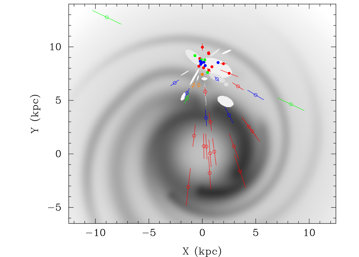
Figure 4: The Milky Way as viewed from the North Galactic Pole, with the Galactic Centre located at the origin of the coordinate system and the Sun at $(0~{}{\rm kpc},~{}8.5~{}{\rm kpc})$. The greyscale represents the distribution of mid-plane electron density from the NE2001 model of Cordes & Lazio (2002) (for clarity, individual high-density clumps are not shown). The data show the projected locations onto the Galactic $(X,Y)$ plane of pulsars with known, reliable, distances. Colours and symbols are as in Figure 1.

In Figure 4 we show the locations of the pulsars in our sample projected onto the Galactic plane, overlaid with the NE2001 electron density model. Of the 15 systems for which $|b|\geq 40^{\circ}$ (shown in blue), six sight lines (all to globular clusters) extend over a significant distance through the Galaxy, traversing several, separate, spiral arms. These data clearly do not probe merely local gas, but are representative of the WIM within several kpc of the Sun. In any case, these sightlines should not be dominated by individual density features, since the long path lengths ensure that individual clumps or cavities in the electron distribution largely average out.

The remaining nine systems (all pulsar parallaxes) lie much closer to the Sun. As indicated in Figure 4, there are several cavities and enhancements in the solar neighbourhood (see Cox & Reynolds 1987; Toscano et al. 1999; Sfeir et al. 1999, and references therein), whose presence could dominate the DM of nearby pulsars, and thus might bias our fits. A qualitative argument against this possibility is that in Figure 1, the envelope defined by the high-$|b|$ parallax data joins smoothly onto that traced out by the high-$|b|$ globular cluster data. Since we have argued above that the DMs to globular clusters trace the widespread properties of the WIM in the disk, the pulsar parallaxes are also consistent with this interpretation.

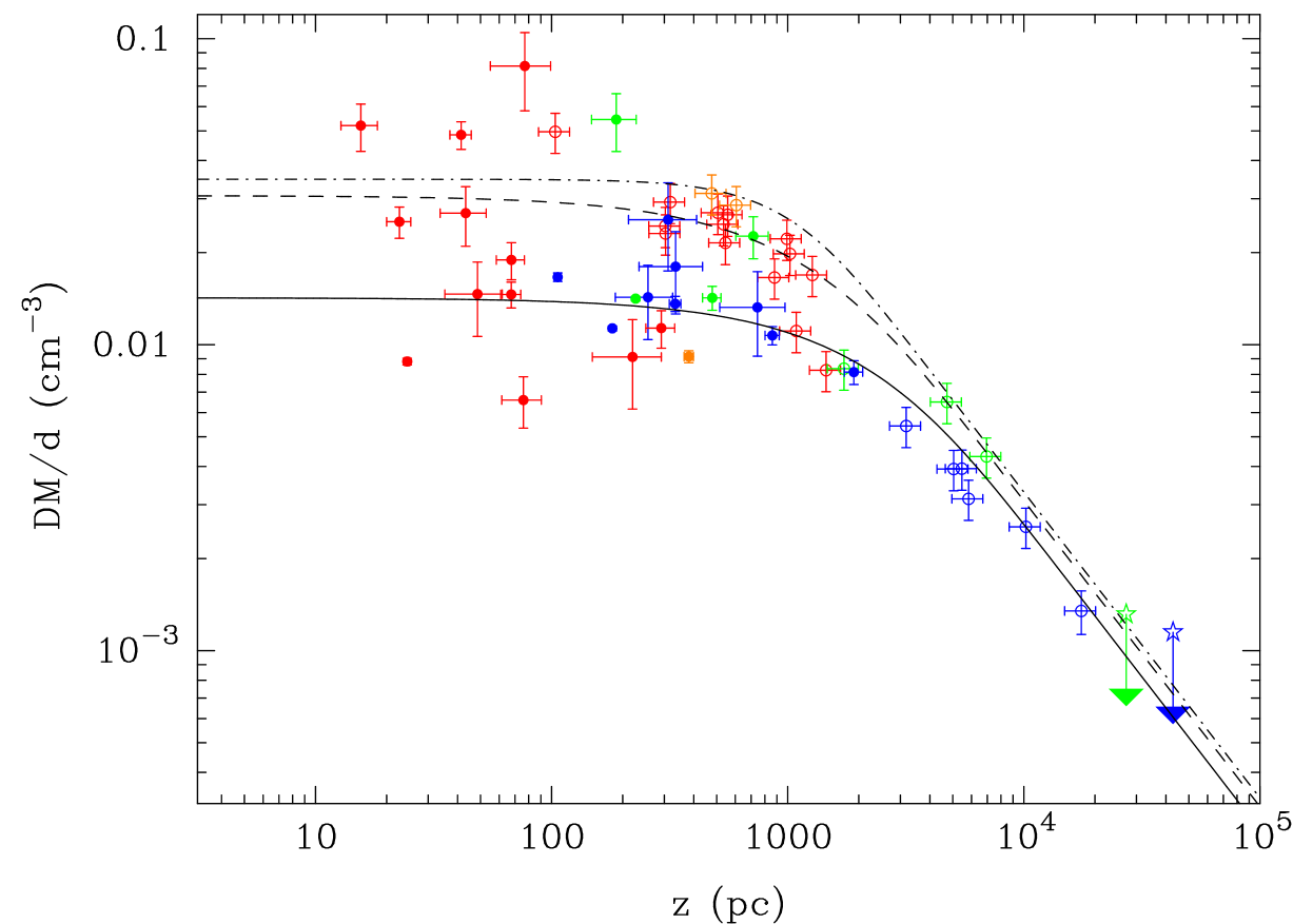
Figure 5: Dispersion measure per unit distance (equivalent to the electron density averaged along the line of sight) as a function of height above the Galactic plane for pulsars with known, reliable, distances. Colours, symbols and curves are as in Figure 1.

We can quantify the effects that local structure might be having on the data by plotting ${\rm DM}/d$ versus $z$, where $d$ is the distance to each source. This distribution is plotted in Figure 5: the electron column per unit distance plotted in the ordinate is equal to the mean electron density along the sightline to a given source. The corresponding predictions for ${\rm DM}(z)/d\equiv{\rm DM}_{\perp}(z)/z$ for each of the curves drawn in Figure 1 are plotted in Figure 5, with the form of ${\rm DM}_{\perp}(z)$ given by Equation (6).

For a generally smooth distribution of electrons in all directions, values of ${\rm DM}/d$ will follow a single curve such as those plotted in Figure 5. Pulsars located inside or just beyond a cavity will exhibit values of ${\rm DM}/d$ that sit below this curve, while pulsars that sit behind density enhancements will have values of ${\rm DM}/d$ above this curve. Both such effects are clearly seen in Figure 5, especially for sources at low $|b|$ (coloured red and orange), which are not included in our best fit. However, if local structure is affecting our data, then high-latitude pulsars (coloured blue) at low values of $z$ should have values of ${\rm DM}/d$ that deviate more from the best fit curve than do data for pulsars at higher $z$. Only for one pulsar (at $z\approx 300$ pc) of the 15 sources in our sample is there a slight suggestion of such an effect. The small errors in $n_{0}$ and $H_{n}$ derived from bootstrapping confirm that these data do not have a significant effect on our overall fit.

From Figures 4 and 5, we conclude that localised structures are not biasing our results, and that the fits to DM data in Figure 1 are a meaningful representation of the ensemble scale height of diffuse ionised gas within several kpc of the Sun.

4.1.2 Local Structure in Emission Measure

Another way in which localised structure may bias our measurements is in our assumption that the scale heights $H_{n^{2}}$ and $H_{n}$ correspond to the same regions. The determination of $H_{n^{2}}$ by Haffner et al. (1999) was specific to a particular segment of the Perseus arm. In contrast, the DM data in Figure 1 represent integrated column densities spread over a factor of $\approx 200$ in $z$ and distributed over a range of Galactic longitudes (see Figs. 2 and 4). Thus while we have argued in §4.1.1 that the DM data represent ensemble properties over several kpc of the Galactic disk, the EM data provide no such guarantees. If ionised gas above the Perseus arm has special properties (and indeed Fig. 4 shows that none of our high-latitude pulsars lie in or behind the Perseus arm), then the conclusions of §3.3 are not correct.

There are two arguments that support the calculations in §3.3. First, Lazio & Cordes (1998a,b) have specifically studied the properties of diffuse ionised gas toward the Perseus arm and over the rest of the outer Galaxy, and conclude that the ionised disk shows neither warping nor flaring in these regions. Second, even if structure peculiar to the Perseus arm might introduce some bias into our calculations, the fundamental result in §3.3 is that $H_{n}/H_{n^{2}}\gg 2$. Only completely different behaviour for the Perseus arm compared to the sightlines in other directions probed by pulsar DMs could reduce this ratio sufficiently to remove the need for a $z$-dependent filling factor. NGC 891 and M31, two spiral galaxies with broadly similar properties similar to the Milky Way, show variations in the thickness of their ionised gas layers as a function of position, but at fractions of no more than $\sim$50% (Rand et al. 1990; Miller & Veilleux 2003; Fletcher et al. 2004).

4.2 Two Cloud Populations?

In §3.3, we assumed that at a given height $z$, WIM clouds can be described by a single volume-averaged electron density, $n(z)$. This is obviously an idealised situation, but is a reasonable approximation of actual data, which suggest that $n(z)$ shows a modest spread in density around a well-defined average value (Hill et al. 2008). In the model considered in §3.3, we have assumed that this simple cloud population produces both the DMs and EMs that we observe. The fact that $H_{n}/H_{n^{2}}\neq 2$ can then be explained by invoking separate dependences of $N$ and $f$ on $z$, as described by Equations (10) & (11).

However, an alternative possibility is that there are (at least) two populations of WIM clouds, with separate densities, filling factors and scale heights. Specifically, if we suppose that one set of clouds has a low density and a high filling factor, while a second cloud population have a much higher density and a much lower filling factor, then observations of DM will only probe the first group, while data on EM will only trace the second (Gould 1971; Heiles 2001). Carrying out a joint analysis of DMs and EMs to infer overall properties of $N$ and $f$, as we have done in §4.2, would then not be meaningful.

We thus now consider whether the data can be validly interpreted in terms of two separate populations of WIM clouds. Suppose that one group of WIM clouds has electron density $N_{A}(z)$, filling factor $f_{A}$ (which is not a function of $z$) and volume-averaged density $n_{A}(z)\equiv f_{A}N_{A}(z)$. The density of these clouds is distributed exponentially, such that $n_{A}(z)$ and $N_{A}(z)$ both have a scale height $H_{A}$. A second cloud population has corresponding parameters $N_{B}(z)$, $f_{B}$ and $n_{B}(z)\equiv f_{B}N_{B}(z)$, with an exponential scale height $H_{B}$.

The vertical dispersion and emission measures integrated through the thick disk then become:

$${\rm DM}_{0}=f_{A}N_{A,0}H_{A}+f_{B}N_{B,0}H_{B}~{},$$ (24)

$${\rm EM}_{0}=f_{A}N^{2}_{A,0}H_{A}/2+f_{B}N^{2}_{B,0}H_{B}/2~{},$$ (25)

respectively, where the subscript “0” indicates extrapolated mid-plane values, and where we have disregarded second order terms in $f_{A}f_{B}$. The observed behaviours of DM and EM with $z$ are both well described by a single exponential layer (Fig. 1; Fig. 4 of Haffner et al. 1999), implying that only a single population of clouds contributes to each set of measurements. We thus adopt the requirement that the DMs only probe population A but that the EMs only probe population B:

$$f_{B}N_{B,0}H_{B}\ll{\rm DM}_{0}~{},$$ (26)

and

$$f_{B}N^{2}_{B,0}H_{B}/2\approx{\rm EM}_{0}.$$ (27)

Comparing Equations (21) & (27), we can then identify $H_{B}/2\equiv H_{n^{2}}$, so that combining Equations (26) & (27) then yields:

$$f_{B}\ll\frac{L_{c}}{4H_{n^{2}}}\approx 0.2,$$ (28)

$$N_{B,0}\gg 2N_{c}\approx 0.15~{}{\rm cm}^{-3},$$ (29)

with $L_{c}$ and $N_{c}$ defined at the end of §3.3. We can rule out the existence of such a component to the diffuse WIM, because H$\alpha$ data lead to direct estimates of mid-plane densities for the diffuse WIM of $N_{B,0}\approx 0.1-0.3$ cm^-3 (Reynolds 1980, 1983; Reynolds et al. 1995). Since the predicted cloud densities of population B are at odds with those observed, we conclude that it is not valid to argue that DMs and EMs are produced by separate populations. The alternative is that the distribution of ionised clouds is described by a single set of parameters, $n(z)\equiv f(z)N(z)$, as laid out in §3.3.

4.3 General Implications

We have shown in §4.1 that our results are not likely to be merely a result of local structure in DM or EM, and we have demonstrated in §4.2 that we have not mistakenly conflated data on two separate populations of ionised clouds. We emphasise that even if some of our arguments in these Sections can be shown to have shortcomings, our main result, that $H_{n}\approx 1.8$ kpc, is derived purely from pulsar DMs, and does not rely on any subsequent assumptions about filling factors or EMs. We now consider some of the implications of our revised WIM parameters.

We first consider the Galactic distribution of pulsars. The most frequent application of models for the WIM is to derive distance estimates of pulsars from measurements of their DMs. Figure 1 demonstrates that the NE2001 model does not correctly reproduce the DMs of high-latitude pulsars at known distances. In turn, it seems likely that the DM-derived distances for many high-$|b|$ pulsars without independent distance constraints may be substantial underestimates; the corresponding predictions from NE2001 should be used with caution. Indeed, Kramer et al. (2003) and Lorimer et al. (2006) found that if distances predicted by NE2001 are applied to the Parkes multibeam pulsars, these sources are then anomalously clustered toward small $z$.

A revision of the distances to high-latitude pulsars would have important implications. Such data play a major role in characterising the population statistics of millisecond (which tend to be found at high $|b|$ due to their large ages), as well as to predict the yields of future pulsar surveys. Recent studies of these issues have all been underpinned by the NE2001 model (e.g., Hobbs et al. 2005; Story et al. 2007), and the corresponding conclusions may now need to be reconsidered. Specifically, if the true distances to high-$|b|$ pulsars are larger than have been assumed in recent studies, then millisecond pulsars may have higher space velocities, be more luminous, and be more numerous than has been previously argued.

Overall, we note that while the NE2001 electron density model most likely underestimates the distances to high-latitude pulsars, one of the major strengths of this model was that it corrected the severe over-estimates that previous models had made for the distances to low-latitude pulsars. Thus it is unwarranted to argue that the entire NE2001 model is unreliable; our analysis focuses only on the high-latitude component, and indicates only that this aspect needs revisiting. Correspondingly, we do not recommend that Equation (6) or Figure 1 be used to estimate the distances or DMs to individual pulsars at high $|b|$, but instead suggest that in future studies, the results derived here should be incorporated into a revised global model for the disk, spiral arms and halo.

As noted in §1.1.1, a full three-dimensional model of Galactic magnetic fields, cosmic rays and thermal electrons, but assuming a warm layer with scale height $H_{n}\sim 1$ kpc, results in an unacceptably high halo magnetic field strength of $\approx 10$ $\mu$G, and an unreasonable truncation of cosmic ray electrons at $z=1$ kpc (Sun et al. 2008). As Sun et al. (2008) explicitly discuss, a WIM layer with a scale height of $\sim 2$ kpc can simultaneously solve both these problems. The independent conclusions that we have arrived at here thus support a relatively weak ($\sim 2$ $\mu$G) magnetic field in the halo, and a cosmic ray distribution which can diffuse to high $z$.

Despite the more consistent overall picture of the WIM that our analysis can potentially provide, we note that even after artificially increasing the errors in $z$ as was carried out in §3.1.1, the best fit in Figure 3 has $\chi^{2}_{r}\approx 5$. The fact that $\chi^{2}_{r}\gg 1$ clearly indicates that a smooth exponential slab is not an accurate description of the individual data points. As discussed extensively by Cordes & Lazio (2002, 2003), many sightlines through the Galaxies pass through intervening regions where the density is either enhanced (clumps) or reduced (voids). These systematic deviations are not incorporated in our model, and imply that $\chi^{2}_{r}$ will always be relatively large in any simple fit to this complex data set. However, it is noteworthy that $\chi^{2}_{r}$ does drop significantly for higher cut-offs in $|b|$ (see Fig. 3), indicating that the WIM becomes more homogeneous as one moves further from the Galactic plane. We further note in Figure 1 that the low-latitude data (in red) are distributed both above and below the fits that include these data (dashed and dot-dashed lines), while the highest latitude data (in blue) generally lie only on or above the corresponding best fit (solid line). This suggests that in the Galactic plane there are both clumps and voids in the WIM, but that far from the plane any deviations from a smooth distribution are mainly in the form of clumps, rather than voids. This same argument produces additional qualitative evidence against the NE2001 model for ionised gas at high $z$. If the NE2001 description (shown as a dot-dashed line in Fig. 1) is correct, then the fact that almost every blue data-point in Figure 1 lies well below this line requires that there be separate voids in electron density in front of all these high-$|b|$ pulsars. A large number of voids to account for all these low DMs does not seem warranted, especially given that these pulsars are distributed at a wide range of distances, in a variety of directions, and sit both above and below the Galactic plane (see Figs. 2 & 4). The sustained low DMs for all these pulsars compared to the NE2001 model suggests that a different overall density distribution is required in these directions.

4.4 Mid-Plane Properties of the Diffuse WIM

In this section, we compare our extrapolated mid-plane values for the thick-disk WIM to other studies of the ISM in the disk. At $z=0$, we infer a volume-averaged density for the diffuse WIM of $n_{0}=0.014\pm 0.001$ cm^-3. Observationally, this can be compared to values of ${\rm DM}/d$ for pulsars at low $|b|$ with known distances, which typically yield $n_{0}\sim 0.03-0.1$ cm^-3 along complicated sightlines through spiral arms, and $n_{0}\approx 0.01-0.02$ cm^-3 in inter-arm regions (Johnston et al. 2001; Weisberg et al. 2008, and references therein). As discussed in §1, this indicates two components for warm ionised gas in the ISM: free electrons associated with individual H ii regions (only found in spiral arms at low $|b|$), and the diffuse, thick-disk WIM (seen at all latitudes and in all directions). We have not included any contribution from the former component in our model, since we only fit DMs at high $|b|$ and high $z$. Thus the fact that observational estimates for $n_{0}={\rm DM}/d$ in inter-arm regions agree well with our derived value for $n_{0}$ supports the picture of an extended diffuse WIM in which individual dense ionised regions are embedded, and suggests that the thick WIM layer extends all the way down into the Galactic plane.

Estimates of $n_{0}$ from previous attempts to globally model the thick-disk WIM are summarised in Table 1. Our value for $n_{0}$ is systematically lower than that in almost all these other studies. In most cases, this results from the fact that ${\rm DM}_{0}\equiv n_{0}H_{n}$ for an exponential slab. Since all studies generally agree on ${\rm DM}_{0}$, but most previous authors have derived much smaller scale heights than we have found, their estimates of $n_{0}$ are correspondingly larger. BMM06 set only a lower limit on $H_{n}$; their estimate of $n_{0}$ may be biased by the systematic distance uncertainties in their analysis, as discussed in §1.1.2.

A variety of studies have also estimated the mid-plane filling factor of the WIM, as summarised in Table 2. The value $f_{0}=0.04\pm 0.01$ which we derived in §3.3 agrees with the estimate of BMM06, but is substantially smaller than that found in most other studies. This discrepancy results from the fact that calculations of $f_{0}$ are usually degenerate with estimates of $n_{0}$ (see, e.g., Eqn. [9] of Reynolds 1991b). In our model, $f_{0}\propto(n_{0})^{2}$ (from Eqn. [23]), and we have explained above that $n_{0}$ needs to be revised downward from previous estimates by a factor of $\sim 1.7-2$. The true value of $f_{0}$ in the WIM must then be a factor of $\sim 3-4$ smaller than what has been found in previous studies, as we have determined here.

Our estimates for $f_{0}$ and $n_{0}$ imply a typical mid-plane density for WIM clouds $N_{0}\equiv n_{0}/f_{0}=0.34\pm 0.06$ cm^-3, which agrees with the theoretical prediction $N_{0}=0.3$ cm^-3 of Cox (2005). Independent estimates of $N_{0}$ have been carried out by Reynolds (1980, 1983) and Reynolds et al. (1995), who measured EMs along a variety of sightlines and found $N_{0}\approx 0.1-0.3$ cm^-3, in reasonable agreement with our value. The thermal pressure of the WIM is $P=2NkT_{e}$, so for $T_{e}\approx 8000$ K (e.g., Reynolds et al. 1999), we infer a mid-plane ISM pressure for the thick-disk WIM of $P_{0}/k\approx 5400\pm 1000$ K cm^-3. Other estimates for the pressure of the WIM and of other ISM phases show a wide variation depending on local conditions, but certainly the above value falls comfortably within the typically observed range (see Cox 2005).

Heiles (2001) argued that there must be two separate components of the diffuse WIM, one which contributes to EMs seen in H$\alpha$, and a second which separately produces the DMs seen for pulsars. We have already shown in §4.2 that, as an overall model for the ISM, a two-phase WIM is not supported by the data. Here we briefly consider the specific arguments made by Heiles (2001). He begins by assuming that the EMs and DMs are produced in the same ISM phase, and then writing $N_{0}=N_{c}\equiv{\rm EM}_{0}/{\rm DM}_{0}$. The implied density leads to an anomalously underpressured WIM compared to the cold, neutral, ISM, a problem which can be relieved by putting the electrons that contribute to EMs and DMs into distinct phases. However, the expression $N_{0}={\rm EM}_{0}/{\rm DM}_{0}$ is only valid for a slab of uniform density; for the exponential fall-off considered here, the appropriate expression is $N_{0}=({\rm EM}_{0}/H_{n^{2}})/({\rm DM}_{0}/H_{n})$, which leads to a WIM pressure $\sim 4-5$ times higher than in the discussion of Heiles (2001). With this correction, there is approximate pressure equilibrium between the WIM and other phases of the ISM, so that a model in which the EMs and DMs are produced by the same gas is sustainable.

Finally, we can combine Equations (16) & (21) to estimate a mean square electron density at midplane $(n^{2})_{0}\equiv{\rm EM}_{0}/H_{n^{2}}=0.005\pm 0.001$ cm^-6. This value, estimated from quantities which we have not substantially revised in this paper, is broadly comparable to previous estimates, as listed in Table 3.

In summary, our results imply that within a few kpc of the Sun, the thick-disk component of the WIM at mid-plane is comprised of clouds of electron density $N_{0}\approx 0.3$ cm^-3 and a volume filling factor of $f_{0}\approx 4\%$, corresponding to a volume-averaged electron density $n_{0}\approx 0.014$ cm^-3. If the diffuse WIM is considered separately from denser gas in the plane associated with discrete H ii regions, these values are in broad agreement with independent estimates made by other approaches. We note that radio recombination line studies generally identify higher values of $N_{0}$ and lower values of $f_{0}$ than what we have derived here (e.g., Heiles et al. 1996b; Roshi & Anantharamaiah 2001), but these emission lines preferentially trace denser gas, possibly associated with the outer envelopes of H ii regions or with the walls of chimneys in the ISM (Anantharamaiah 1986; Heiles et al. 1996b).

4.5 Anti-Correlation of $N$ and $f$, and Evolution of WIM Properties with $z$

The total mass and ionisation rate of the WIM are unchanged in our analysis compared to previous estimates (e.g., Reynolds 1990b), since the calculations of these quantities primarily depend on the integrated column densities EM₀ and DM₀, rather than on the scale-height. What the calculations in §3.3 do imply is contrasting behaviours for the cloud density, $N$, and the locally averaged electron density, $n$, as a function of height above the Galactic plane. The former decays over a relatively small scale height, $\approx 500$ pc. But the volume filling factor, $f$, of these ionised clouds increases as one moves further from the plane, counter-balancing the decreasing internal cloud density. Since $f$ increases with $z$ at a rate slightly more slowly than that with which $N$ decays, $n\equiv fN$ decays relatively slowly as a function of $z$. These results agree with the earlier findings of BMM06, who through a separate approach derived broadly comparable values of $H_{N}$ and $H_{f}$ to those found here, albeit with much larger uncertainties (compare Eqn. [2] with Eqns. [19] & [20]).

An important distinction between our analysis and that of BMM06 is that we find $H_{N}<H_{f}$, while BMM06 concluded that $H_{N}\approx H_{f}$. As per Equation (14), BMM06 thus could infer only a lower limit on $H_{n}$, and indeed they argued that there is no evolution in $n$ for $0<z<1$ kpc, based on the constancy of ${\rm DM}/d$ over this range. However, as discussed in §1.1.2, there are large uncertainties in the values of $d$ and $z$ used in their analysis. Figure 5 shows that for our sub-sample of pulsars with reliable distances and with $|b|\geq 40^{\circ}$, there is a gradual decline in ${\rm DM}/d$ with increasing $z$ up to $z\approx 1$ kpc, which joins smoothly to the behaviour seen for $z\gg 1$ kpc (note that the scatter for the blue points in Fig. 5 is much smaller than for the equivalent plot in Fig. 12 of BMM06). This can only occur if $n$ steadily decays with $z$, requiring $H_{N}<H_{f}$ as we have inferred above.

The decaying exponential for $N$ compared to the growing exponential in $f$ obviously implies an overall anti-correlation between $f$ and $N$, as has also been found through various other approaches (Pynzar’ 1993; Berkhuijsen 1998; Berkhuijsen & Müller 2008, BMM06). For a dependence:

$$f(N)=\beta\left(\frac{N}{{\rm cm}^{-3}}\right)^{\alpha},$$ (30)

we can combine Equations (10), (11), (19), (20), (22) & (23) to derive $\alpha=-0.73^{+0.06}_{-0.03}$ and $\beta=0.018\pm 0.004$. This determination differs substantially from $\alpha=-1.07\pm 0.03$ found by BMM06, but agrees with $\alpha\approx-0.7$ as derived by Pynzar’ (1993). Since $\alpha\equiv-H_{N}/H_{f}$, the discrepancy between our estimate and that of BMM06 simply results from our finding that $H_{N}<H_{f}$ as discussed above.

BMM06 consider two possible physical interpretations of Equation (30) (see also discussion by Berkhuijsen & Müller 2008): either it can represent a stochastic, turbulent ensemble of clouds of different sizes and different densities, or it describes the equation of state of ionised clouds, in that it probes the response of the WIM to a change in external conditions. In the situation that we consider here, the variation of $f$ and $N$ are both modeled as smooth functions of $z$, so the latter case applies.

In this context, what is the physical significance of the anti-correlation between $N$ and $f$, and of the differing scale heights for these two quantities? We first note that the thermal gas pressure, $P=2NkT_{e}$, depends on $N$ but not on $f$. If the evolution of $T_{e}$ with $z$ is modest (Reynolds et al. 1999; Peterson & Webber 2002), then the pressure decays exponentially with a scale height $H_{N}\sim 500$ pc, as described by Equation (11). This agrees well with the pressure scale height derived from hydrostatic equilibrium calculations of the full multi-phase ISM (Boulares & Cox 1990; Ferrière 1998a).

To interpret the evolution of $f$ with $z$, we consider the simple case in which the WIM is composed of a large number of clouds, all with the same number of electrons per cloud, $\mathcal{N}$, and with $Cdz$ clouds contained in a vertical interval $dz$. The volume of an individual cloud is $V(z)$, so that $N(z)=\mathcal{N}/V(z)$. If the total surface area of the Galaxy (assumed to be independent of $z$) is $\Sigma$, then $f(z)=CV(z)/\Sigma=(C\mathcal{N}/\Sigma)N(z)^{-1}$. The exponential decay of $N(z)$ must then imply matching exponential growth in $V(z)$ and in $f(z)$: clouds will be proportionally larger in regions where the ambient pressure is lower. This case corresponds to $\alpha=-1$ (i.e., $H_{N}=H_{f}$), as claimed for the WIM by BMM06.

We can now generalise the above scenario, and allow $C$ and $\mathcal{N}$ to both evolve with $z$. If $\alpha=-1$, then $\mathcal{N}(z)\propto C(z)^{-1}$, i.e., individual clouds at $z=z_{1}$ might contain more electrons than those at $z=z_{2}$, but in this case the total number of clouds at $z_{1}$ will be smaller than that at $z_{2}$ by the same factor. The total mass of the WIM remains constant as a function of $z$.

Now consider the case we have derived here, with $\alpha=-0.73$ (and $H_{N}<H_{f}$). The fact that $\alpha>-1$ indicates that a cloud of a given electron content will be larger in a region of low pressure compared to one under high pressure, but that the increase in size will be less than that expected from the ratio of pressures alone. This could be due to $T_{e}$ decreasing with $z$, but this would, if anything, be opposite to the observed trend (Reynolds et al. 1999). The alternative is that $C(z)\mathcal{N}(z)$ is decreasing with $z$, i.e., the total particle content of the ensemble of clouds (and hence the mass of the WIM) at high $z$ is smaller than for those at low $z$. Quantitatively, we can write $n(z)\equiv f(z)N(z)=C(z)\mathcal{N}(z)/\Sigma$. Equation (5) then implies that $\mathcal{N}(z)C(z)\propto e^{-z/H_{n}}$. We interpret this as the increasing scarcity of warm gas at higher $z$, tracing the transition from the WIM into the hot halo. Electrons at the surface of WIM clouds are heated to $10^{5}-10^{6}$ K via thermal conduction (Cowie & McKee 1977; Vieser & Hensler 2007); they then no longer emit in H$\alpha$, and have too low a density to be seen in pulsar dispersions (see §4.6 below). Such material is thus no longer observable through the DMs or EMs considered in §3.

The implication of the above discussion is that of the various parameters ($H_{n}$, $H_{n^{2}}$, $H_{N}$, $H_{f}$, $\alpha$, $\beta$) that we have used to describe the behaviour of the WIM as a function of $z$, the two quantities that best encapsulate the physical conditions of the gas are $H_{N}$ and $H_{n}$. The former traces the approximate fall in gas pressure away from mid-plane, as moderated by the gravity of the disk and by the effects of magnetic and cosmic-ray pressure. Separately, the latter reveals the extent to which the WIM permeates into the halo, and so probes the lifetimes of warm clouds embedded in hot coronal gas. Since these are two separate physical processes, it is unsurprising that they have distinct scale heights. The fact that $H_{N}\neq H_{n}$ then demands the existence of a third scale height, $H_{f}$, which describes the geometry and size that clouds adopt as they accommodate external pressure but at the same time evaporate.

4.6 Constraints on Hot Coronal Gas

At significant distances from the Galactic plane ($z\stackrel{{\scriptstyle>}}{{{}_{\sim}}}2000$ pc), theory predicts that $\stackrel{{\scriptstyle>}}{{{}_{\sim}}}90\%$ of the ISM by volume should be occupied by $10^{5}-10^{6}$ K coronal gas (Ferrière 1998b; Korpi et al. 1999; de Avillez 2000). To interpret our data at these heights above the plane, we first must determine whether free electrons associated with coronal gas can contribute significantly to the observed DMs (Wolfire et al. 1995; Bregman & Lloyd-Davies 2007), or whether we are only probing the WIM.

The standard picture of the Galactic halo is an extended high-$z$ region of very low electron density, $n_{halo}\stackrel{{\scriptstyle<}}{{{}_{\sim}}}10^{-3}-10^{-4}$ cm^-3 (e.g., Sembach et al. 2003; Yao & Wang 2005). We can test for the presence of such gas in our DM data by attempting a linear fit of DM$.\sin|b|$ vs. $z$ to the data in Figure 1 (and relaxing the previous constraint that $|b|\geq 40^{\circ}$), but only considering systems for which $z>5000$ pc, where the contribution from the WIM should be small. The best fit slope to these six measurements is consistent with zero; bootstrapping provides a $3\sigma$ upper limit on the halo density $n_{halo}<7.6\times 10^{-4}$ cm^-3. We conclude that any contribution to pulsar DMs from hot, low density gas in the halo is below our detection limit.

An independent insight into the relative contributions of the WIM and corona to pulsar DMs comes from the study of Howk et al. (2003, 2006), who compared a variety of ISM tracers, including pulsar DMs, in the foreground of the globular cluster NGC 5272 (Messier 3). NGC 5272 contains four radio pulsars, and corresponds to the blue data point with $z=10.2$ kpc, DM$.\sin|b|=25.9$ pc cm^-3 in Figure 1. Howk et al. (2006) compute separate electron column densities along this sight line for the WIM, for $\sim 10^{5}$ K coronal gas and for $\sim 10^{6}$ K coronal gas. The total DM inferred from pulsar observations is $26.4\pm 0.3$ pc cm^-3 (Hessels et al. 2007), of which Howk et al. (2006) estimate that the WIM contributes $\sim 25$ pc cm^-3 while $10^{5}$ K gas contributes $\sim 1.5$ pc cm^-3. Any remaining contribution from $10^{6}$ K gas must be small: Howk et al. (2006) adopt a model in which this gas has an average electron density of $2.4\times 10^{-4}$ cm^-3. The DM contribution from the globular cluster itself is expected to be negligible (Freire et al. 2001; Howk et al. 2003). These results confirm that almost the entire electron column out to high $z$ originates in warm gas, at an electron temperature $\sim 10^{4}$ K. The pulsar DMs in Figure 1 thus predominantly trace the WIM, and do not constrain the properties of hotter, coronal gas.

4.7 Warm Ionised Gas in the Galactic Halo

Given that our data do not appear to be substantially contaminated by coronal gas, we can now consider what our results imply for the filling factor and pressure of the WIM at high $z$.

The physical requirement that $f\leq 1$ implies that Equation (10) and the results that follow are not well-defined for heights $z\stackrel{{\scriptstyle>}}{{{}_{\sim}}}2200\pm 300$ pc. The value $H_{n^{2}}=400\pm 30$ pc has been derived from H$\alpha$ data in the range $6^{\circ}\leq|b|\leq 35^{\circ}$ (Haffner et al. 1999), which at the distance to the Perseus arm corresponds to a maximum height $z=1400$ pc. The EM data used to derive the dependence of $f$ on $z$ thus fall in the regime where $f\leq 1$, so that our approach is internally self-consistent. At the top of this layer, we find $f=0.30$, $N\approx 0.022$ cm^-3 and $n\equiv fN\approx 0.0065$ cm^-3. This agrees with the findings of BMM06, who argue that $f(z)$ reaches a maximum value $f\approx 0.3$ at $z\approx 1$ kpc. However, this calculation contrasts with previous claims that the WIM is the dominant phase of the ISM at $z\sim 1$ kpc (e.g., Reynolds 1989, 1991a). While the WIM probably dominates over neutral gas in these regions, at this height coronal gas already occupies most of the volume of the ISM (e.g., Korpi et al. 1999).

Beyond the top of the WIM layer studied by WHAM in the Perseus arm, Equation (11) cannot be meaningfully interpreted, since we no longer have independent constraints on both $n$ and $n^{2}$. However, we can broadly characterise the pressure and filling factor of the WIM at high $z$ by noting that $P\propto N\propto n/f$. At large $z$, we know that $n$ continues to decay at least as fast as the exponential in Equation (5), because of the high quality of the fits of this model to the data in Figures 1 & 5 (for $z\stackrel{{\scriptstyle>}}{{{}_{\sim}}}5$ kpc, we cannot rule out the possibility that $n$ begins to fall off more rapidly). While $f$ appears to increase with distance from the mid-plane at low values of $z$, this function must turn over at $z\stackrel{{\scriptstyle>}}{{{}_{\sim}}}2000$ pc to accommodate coronal gas (e.g., Korpi et al. 1999; de Avillez 2000). If $n$ and $f$ are both decreasing functions at high $z$, then $N\equiv n/f$ at these heights must become increasingly larger than predicted by Equation (11). This then implies that any warm ionised gas at high $z$ is over-pressured relative to the exponential decay in pressure seen within 2 kpc of the mid-plane. This high pressure is consistent with the expectation that any small warm clouds at these heights should be enveloped in a hot halo (e.g., Fox et al. 2005).

At $z\approx 5-10$ kpc, the ambient pressure in the Galactic halo is $P/k\approx 1000-2000$ K cm^-3 (Shull & Slavin 1994; Sternberg et al. 2002; Everett et al. 2008). If we assume $T_{e}\approx 10^{4}$ K for the WIM, and adopt Equation (5) as an upper limit on $n$ at these values of $z$, we infer $f<0.02$ for any warm ionised gas at these heights above the plane. These small cloudlets may correspond to the “drizzle” of ionised gas accreting into the halo proposed by Bland-Hawthorn et al. (2007), or to the extraplanar droplets and clumps of H$\alpha$ seen in observations of some edge-on spiral galaxies (Ferguson et al. 1996; Cecil et al. 2001).

5 Conclusion

We have used the dispersion measures of pulsars at known, reliable, distances and the emission measures traced by diffuse H$\alpha$ emission to re-evaluate the structure and distribution of the thick disk of warm ionised gas in the Milky Way. Our main conclusions are as follows:

1. The DMs of high-latitude pulsars are well fit by a plane-parallel distribution of free electrons, in which the volume-averaged electron density, $n$, decays exponentially with height, $z$, above the Galactic plane.

2. Within a few kpc of the Sun, the exponential scale height for $n$ is $H_{n}\approx 1800$ pc, approximately double the value determined in most previous studies. Estimates of distances to high-latitude pulsars using the “NE2001” electron model of Cordes & Lazio (2002, 2003) are thus likely to be substantial underestimates.

3. Within a few kpc of the Sun, the mid-plane volume-averaged electron density of the diffuse WIM is $n_{0}=0.014\pm 0.001$ cm^-3, and the corresponding total vertical column density of the WIM is $\approx 26$ pc cm^-3. Assuming a total vertical emission measure EM${}_{0}=1.9\pm 0.3$ pc cm^-3, clouds in the thick-disk component of the WIM have a typical internal electron density of $N_{0}=0.34\pm 0.06$ cm^-3 at mid-plane, with a volume filling factor $f_{0}=0.04\pm 0.01$.

4. Comparison of DMs and EMs shows that the internal electron density, $N$, of individual ionised clouds within the thick-disk WIM decays rapidly with $z$, with an exponential scale height $H_{N}\approx 500$ pc. The differing behaviour for $H_{n}$ and $H_{N}$ requires that the filling factor of the WIM grows exponentially with $z$ over the range $0\leq z\stackrel{{\scriptstyle<}}{{{}_{\sim}}}1.4$ kpc, with a scale height $H_{f}\approx 700$ pc.

5. The filling factor of the thick-disk WIM probably reaches a maximum of $f\approx 0.3$ at $z\approx 1.5$ kpc. At larger distances from the Galactic plane, the ISM becomes increasingly dominated by hotter, coronal, gas in the halo. However, hot low-density halo gas makes only a negligible contribution to observed pulsar DMs.

A variety of future observations will allow us to test the above conclusions, and to better understand the structure of the diffuse WIM. Most immediately, from late 2008 WHAM will be relocated to the southern hemisphere, allowing studies similar to those carried out on the Perseus spiral arm to now be repeated for other regions.

Further improvements will come from an increase in the number of high-latitude radio pulsars with direct distance estimates. For example, only $\approx 25\%$ of the Galactic globular clusters at $|b|\geq 40^{\circ}$ contain known radio pulsars. While some clusters at these latitudes have been searched for pulsations without success (Anderson 1993; Biggs & Lyne 1996; Hessels et al. 2007), at least some of these targets probably contain as yet undetected pulsars (e.g., NGC 5634; Sun et al. 2002), and should be searched more deeply. Furthermore, there are several high-latitude pulsars with 1.4 GHz radio fluxes at the level of a few mJy, which is sufficiently bright to derive interferometric parallaxes through future observations.

Most surveys for radio pulsars have concentrated on the Galactic plane, and those surveys that have covered high-latitude regions have been of comparatively modest sensitivity (e.g., Manchester et al. 1996). Forthcoming all-sky pulsar surveys with more sensitive instrumentation will greatly expand the sample of high-$|b|$ pulsars, whose DMs can then be used to better map out the structure of the WIM.

Finally, we note that the new model we have presented for the WIM can also be used to probe Galactic magnetic fields at high $z$. In a subsequent paper, we will combine the density distribution derived here with Faraday rotation measures of a large number of polarised extragalactic sources at high $|b|$, with which we aim to derive the strength and geometry of magnetic fields in the Galactic halo.

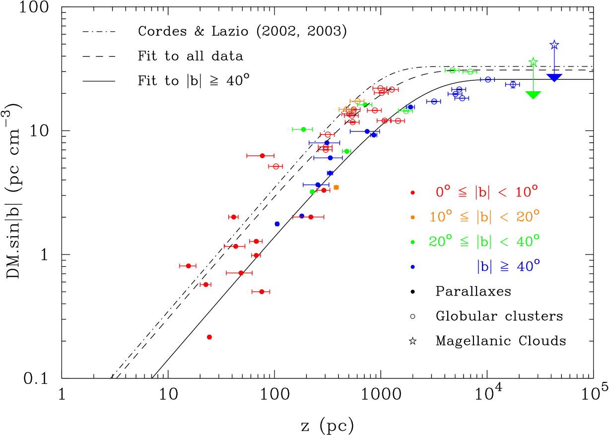
Figure 1: Distribution of dispersion measure as a function of height above the Galactic plane for pulsars with known, reliable, distances. Pulsars with distance determinations from trigonometric parallaxes, from associations with globular clusters and from associations with the Magellanic Clouds are shown as filled circles, open circles and stars, respectively (data for the Magellanic Clouds are indicated as upper limits, since the Galactic and Magellanic DM contributions cannot be separated). Data are colour-coded according to the magnitude of their Galactic latitude, $|b|$, as indicated in the legend. The error bars represent the published uncertainties. The three curves represent planar slabs of ionised gas with a scale height $H_{n}$ for the volume averaged electron density, $n$. The dot-dashed line shows a $n\propto{\rm sech}^{2}(z/H_{n})$ density dependence, using the parameters given in Table 3 of Cordes & Lazio (2002) (see also Fig. 1 of Cordes & Lazio 2003); the dashed line shows the best fit for an exponential slab ($n\propto e^{-z/H_{n}}$) to all the data in the figure; the solid line shows the best exponential fit to only those data for which $|b|\geq 40^{\circ}.$

Figure 3: Best fit parameters for a planar slab of ionised gas with an exponential scale height, as a function of the minimum cut-off used for $|b|$. The top, centre and bottom panels show the scale height, $H_{n}$, the extrapolated mid-plane electron density, $n_{0}$, and the reduced $\chi^{2}$ of the fit, $\chi^{2}_{r}$, respectively. In the top two panels, the dot-dashed line shows the parameters given in Table 3 of Cordes & Lazio (2002), while the error bars show the 68% confidence intervals on each parameter. In the bottom panel, the number above each datum indicates the number of points from Figure 1 used in the fit. The fit did not converge for a cut-off $|b|_{\rm min}=10^{\circ}$.

Table 1: Estimates of the scale height and mid-plane value of the volume-averaged electron density in the thick-disk component of the WIM. The entries have been sorted by increasing scale height.

$H_{n}$ (pc)	$n_{0}$ (cm-3)	Reference	Comment
$430-670$	$0.028-0.035$	Readhead & Duffett-Smith (1975)
$670^{+170}_{-140}$	$0.033\pm 0.002$	Nordgren et al. (1992)
$83$0	$0.025\pm 0.005$	Peterson & Webber (2002)
$880\pm 60$	$0.019$	Taylor & Cordes (1993)	Thick-disk component of two-component model
$890^{+250}_{-180}$	$0.036$	Savage et al. (1990)
$900$	$0.025$	Reynolds (1991a)	Thick-disk component of two-component model
$930\pm 130$	$0.023\pm 0.004$	Berkhuijsen & Müller (2008)
$950$	$0.035$	Cordes & Lazio (2002)	Thick-disk component of two-component model
$>1000$	$0.025$	Lyne et al. (1985)	Thick-disk component of two-component model
$>1000$	$0.021\pm 0.001$	BMM06
$1070-1100$	$0.018-0.020$	Gómez et al. (2001)	Thick-disk component of two-component model
$1830^{+120}_{-250}$	$0.014\pm 0.001$	This paper	Only uses data at $|b|\geq 40^{\circ}$

Table 2: Estimates of the mid-plane volume filling factor of the WIM (sorted by decreasing $f_{0}$).

$f_{0}$	Reference
$0.2$	Cordes et al. (1991)
$0.11$	Peterson & Webber (2002)
$0.1-0.5$	Pynzar’ (1993)
$0.1-0.2$	Reynolds (1991b, 1997)
$0.1$	Kulkarni & Heiles (1987, 1988)
$0.083$	Cox (2005)
$0.05-0.14$	Ferrière (2001)
$0.08\pm 0.02$	Berkhuijsen & Müller (2008)
$0.05\pm 0.01$	BMM06
$0.04\pm 0.01$	This paper

Table 3: Estimates of the mid-plane mean square electron density of the WIM (sorted by decreasing $(n^{2})_{0}$).

$(n^{2})_{0}$ (cm-6)	Reference
$0.009$	Kulkarni & Heiles (1987)
$0.008\pm 0.001$	BMM06
$0.007$	Reynolds (1990a)
$0.005-0.012$	Ferrière (2001)
$0.005\pm 0.001$	Berkhuijsen & Müller (2008)
$0.005\pm 0.001$	This paper

References

- Alves (2004) Alves, D. R. 2004, New Astron. Rev., 48, 659
- Anantharamaiah (1986) Anantharamaiah, K. R. 1986, J. Astrophys. Astr., 7, 131
- Anderson (1993) Anderson, S. B. 1993, PhD thesis, California Institute of Technology
- Backer (1974) Backer, D. C. 1974, ApJ, 190, 667
- Berkhuijsen (1998) Berkhuijsen, E. M. 1998, in The Local Bubble and Beyond (IAU Colloquium No. 166), ed. D. Breitschwerdt, M. J. Freyberg, & J. Trümper (Springer-Verlag), 301–304
- Berkhuijsen et al. (2006) Berkhuijsen, E. M., Mitra, D., & Müller, P. 2006, Astron. Nach., 327, 82 (BMM06)