BAT - The Bayesian Analysis Toolkit

Abstract

We describe the development of a new toolkit for data analysis. The analysis package is based on Bayes’ Theorem, and is realized with the use of Markov Chain Monte Carlo. This gives access to the full posterior probability distribution. Parameter estimation, limit setting and uncertainty propagation are implemented in a straightforward manner. A goodness-of-fit criterion is presented which is intuitive and of great practical use.

1 Introduction

The goal of data analysis is to compare model predictions with data, and draw conclusions either on the validity of the model as a representation of the data, or on the possible values for parameters within the context of a model. The paradigm for our data analysis package is shown in Fig. 1. Here, the model $M$ can range from a model purporting to represent nature (e.g., the Standard Model in particle physics) to a simple parametrization of data useful for making predictions or for summarizing data.

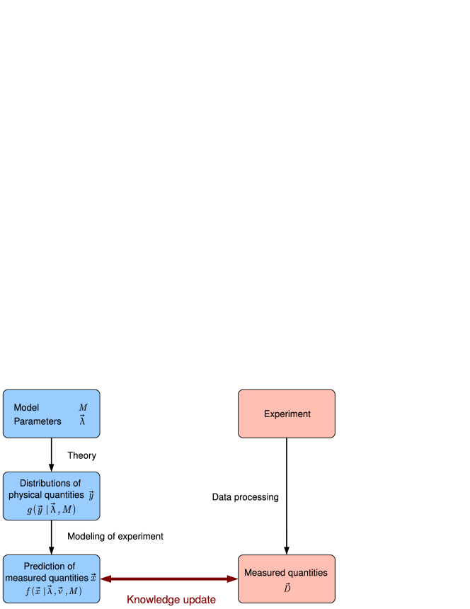
Figure 1: Paradigm for data analysis. Knowledge is gained from a comparison of model predictions with data. Intermediate steps may be necessary, e.g., to model experimental conditions.

1.1 Modeling

The theory or model can be used to provide direct probabilities; i.e., relative frequencies of possible outcomes of the results were one to reproduce the experiment many times under identical conditions. This is possible because the model is a mathematical construction which allows the calculation (or simulation) of frequencies of outcomes. The predictions from the model cannot usually be directly compared to experimental results. An additional step is needed, either to modify the predictions to allow for the experimental effects, or to undo the experimental effects from the data. Obviously, an accurate description of the experimental effects is necessary to produce reliable conclusions.

The function $g(\vec{y}|\vec{\lambda},M)$ gives the relative frequency of getting result $\vec{y}$ assuming the model $M$ and parameters $\vec{\lambda}$. It should satisfy:

$$g(\vec{y}|\vec{\lambda},M)\geq 0$$ (1)

and

$$\sum_{i}g(y_{i}|\vec{\lambda},M)=1\;\;\;\;{\rm or}\;\;\;\;\;\int g(\vec{y}|\vec{\lambda},M)\,d\vec{y}=1$$ (2)

depending on whether discrete or continuous values are measured. In the following, we will write formulae for the continuous case; the modification for the discrete case will be clear. Note that the normalization requirement is often discarded when only relative probabilities of outcomes are needed.

The modeling of the experiment will usually add extra parameters and assumptions. We will use the symbol $\vec{\nu}$ to represent these additional (nuisance) parameters. There could also be additional information not included explicitly in the model which could limit values of the model parameters. This information is often denoted with an additional symbol, e.g., $I$, and we would then have $f(\vec{x}|\vec{\lambda},\vec{\nu},M,I)$ for the frequency distribution of observable quantities $\vec{x}$. We will drop the $I$ in the following - it is assumed everywhere that all available information is used in the probability distributions.

As an example, one can consider the radioactive decay of an unstable nucleus. The model is an exponential decay time distribution, $P(t|\tau)=\frac{1}{\tau}e^{-t/\tau}$, with the lifetime parameter $\tau$. Then

$$g(\{t_{i}\}|\tau)=\prod_{i}P(t_{i}|\tau)=\prod_{i}\frac{1}{\tau}e^{-t_{i}/\tau}\,.$$

We can imagine that we are measuring a sample of nuclei, and that our detector is not able to distinguish two decays which occur too closely in time. Also, the decay times will be measured with some precision which could be modeled with a Gaussian smearing with width $\sigma_{t}$. This measurement resolution may not be known precisely, and could be considered a nuisance parameter. The probability density for a given set of measured times $f(\{t_{j}^{\rm measured}\}|\tau,\sigma_{t})$ could then be determined from a simulation which includes the dead time and measurement resolution.

In general, the judgment on the validity of a model and the extraction of values of the parameters within the model will be based on a comparison of the data, $\vec{D}$, with $f(\vec{x}|\vec{\lambda},\vec{\nu},M)$.

1.2 Formulation of the Learning Rule

The probability of a model, $M$, will be quantified as $P(M)$, with

$$0\leq P(M)\leq 1$$ (3)

while the probability density of the parameters are typically continuous functions. The parameters from the modeling of the experimental conditions are not correlated to the parameters of the physical model so that

$$P(\vec{\lambda},\vec{\nu}|M)=P(\vec{\lambda}|M)P(\vec{\nu})\;\;.$$ (4)

The probability densities satisfy

$$P(\vec{\lambda}|M) \geq 0$$ (5)

$$\int P(\vec{\lambda}|M)\,d\vec{\lambda} = 1$$ (6)

and similarly

$$P(\vec{\nu}) \geq 0$$ (8)

$$\int P(\vec{\nu})\,d\vec{\nu} = 1\;\;.$$ (9)

In the Bayesian approach, the quantities $P(M)$ and $P(\vec{\lambda}|M)$ are treated as probabilities (probability densities), although they are not in any sense frequency distributions and are more accurately described as degrees-of-belief [1]. This degree-of-belief is updated by comparing data with the predictions of the models. The parameter and model degrees-of-belief are the interesting quantities since they contain our knowledge about nature. The purpose of performing experiments is then to modify our degree-of-belief. $P(M)=1$ represents complete certainty of $M$ being correct, and $P(M)=0$ represents complete certainty that $M$ is false.

The procedure for learning from experiment is:

$$P_{i+1}(\vec{\lambda},\vec{\nu},M|\vec{D})\propto f(\vec{x}=\vec{D}|\vec{\lambda},\vec{\nu},M)P_{i}(\vec{\lambda},\vec{\nu},M)\,,$$ (10)

where the index on $P$ represents a state-of-knowledge.

In order to satisfy our normalization requirement

$$\sum_{M}\int P(\vec{\lambda},\vec{\nu},M)\,d\vec{\lambda}\,d\vec{\nu}=\sum_{M}P(M)\left[\int P(\vec{\lambda}|M)\,d\vec{\lambda}\int P(\vec{\nu})\,d\vec{\nu}\right]=1$$ (11)

we have

$$P_{i+1}(\vec{\lambda},\vec{\nu},M|\vec{D})=\frac{f(\vec{x}=\vec{D}|\vec{\lambda},\vec{\nu},M)P_{i}(\vec{\lambda},\vec{\nu},M)}{\sum_{M}\int f(\vec{x}=\vec{D}|\vec{\lambda},\vec{\nu},M)P_{i}(\vec{\lambda},\vec{\nu},M)\,d\vec{\lambda}\,d\vec{\nu}}\;\;.$$ (12)

We usually just write $P_{i}=P_{0}$, and this quantity is called the prior. It contains all information we may have on the model and parameter values before the experiment is performed. The posterior probability density function, $P_{i+1}$, is usually written simply as $P$. It describes the state of knowledge after the experiment is analyzed.

For a given model, $M$, $f$ is a function of the model parameters, the experimental parameters, and the possible outcomes $\vec{x}$. When $f$ is viewed as a function of $(\vec{\lambda},\vec{\nu})$ for fixed $\vec{x}=\vec{D}$, it is known as the likelihood. In our formulation, $f$ is the relative frequency of a particular result $\vec{x}=\vec{D}$ from our modeling. If $f$ is normalized, we can write

$$P(\vec{D}|\vec{\lambda},\vec{\nu},M)=f(\vec{x}=\vec{D}|\vec{\lambda},\vec{\nu},M)\;\;.$$ (13)

The denominator in Eq. (12) is the probability to get the data, $\vec{D}$, assuming the models $M$ and the description of the experimental conditions describe all possible outcomes, and can be written as $P(\vec{D})$. Using this notation, we then recover the classic equation due to Bayes:

$$P(\vec{\lambda},\vec{\nu},M|\vec{D})=\frac{P(\vec{D}|\vec{\lambda},\vec{\nu},M)P(\vec{\lambda},\vec{\nu},M)}{P(\vec{D})}\;.$$ (14)

The scheme for updating knowledge, as written down here, is general and straightforward. There can be difficulties in implementation when dealing with multi-dimensional spaces, and the toolkit presented here is designed to help the user solve these technical issues. It is up to the user to carefully define the function $f$ as well as the priors. The precision and accuracy of the results will depend primarily on the quality of the inputs. Given that these functions are well-defined, the BAT program will then be useful as a tool for model testing and parameter estimation.

In the following, we start with a discussion on how to perform parameter estimation with the model fixed. This is followed with a discussion of goodness-of-fit criteria, and the closely related topic of model comparison. Discovery criteria are discussed in this context. Setting limits on parameters while keeping the model fixed is briefly discussed. We then switch to the practical realization of this analysis framework in terms of Markov Chains. A brief review of Markov Chains is given, followed by a discussion of the implementation in BAT. We then give examples of parameter estimation and model testing to make the ideas more concrete.

2 Parameter Estimation

Parameter estimation is performed while keeping the model fixed. In this case, we write

$$P(\vec{\lambda},\vec{\nu}|\vec{D},M)=\frac{P(\vec{x}=\vec{D}|\vec{\lambda},\vec{\nu},M)P_{0}(\vec{\lambda},\vec{\nu}|M)}{\int P(\vec{x}=\vec{D}|\vec{\lambda},\vec{\nu},M)P_{0}(\vec{\lambda},\vec{\nu}|M)\,d\vec{\lambda}\,d\vec{\nu}}\;\;.$$ (15)

The output of the evaluation is a normalized probability density for the parameters, including all correlations. This output can be used to give best-fit values, probability intervals for the parameters, etc.

The function, $P(\vec{x}=\vec{D}|\vec{\lambda},\vec{\nu},M)$, which gives the probability density at $\vec{x}=\vec{D}$ given the model $M$ and the parameters $(\vec{\lambda},\vec{\nu})$ must be defined by the user, and must return reasonable values for all possible data results. This likelihood function contains the information both from the theory input as well as the modeling of the experimental conditions. It must be defined case-by-case. Similarly, the prior probabilities, $P_{0}(\vec{\lambda},\vec{\nu}|M)$, must be defined by the user. These prior probability functions define the range over which the parameters can vary, and any preconceptions concerning their possible values. Note that if these priors are set to a constant (not always applicable!), then the parameter estimation using the mode of the posterior probability density function (pdf) is equivalent to a maximum likelihood estimation. If in addition the fluctuations of the data from the model predictions are assumed to follow Gaussian distributions, then the mode finding reduces to a $\chi^{2}$ minimization. The formalism therefore contains these commonly used fitting approaches. It is however completely general and is not limited by these conditions. In all cases, the full posterior pdf is available, thus allowing the user to study correlations between parameters, to perform the propagation of uncertainties without approximations, and to define uncertainty bands or limits as desired. The usefulness of this information is demonstrated in the examples section.

When working with the posterior pdf, $P(\vec{\lambda},\vec{\nu}|\vec{D},M)$, it is often the case that one is interested not in the full pdf, but in the probability distribution for only one, or a few, parameters. These distributions are determined via marginalization. For example, the probability distribution for parameter $\lambda_{i}$ is:

$$P(\lambda_{i}|\vec{D},M)=\int P(\vec{\lambda},\vec{\nu}|\vec{D},M)\,d\vec{\lambda}_{j\neq i}\,d\vec{\nu}\;.$$ (16)

Note that the parameter values which maximize the full posterior pdf usually do not coincide with the values which maximize the marginalized distributions.

2.1 Use of the Posterior Probability Distribution

The posterior pdf, $P(\vec{\lambda},\vec{\nu}|\vec{D},M)$, can be used to evaluate any desired quantity related to the parameters. For example, commonly used quantities are:

Mean of $\lambda_{i}$

$$<\lambda_{i}>=\int P(\lambda_{i}|\vec{D},M)\lambda_{i}\,d\lambda_{i}\;\;.$$

Median of $\lambda_{i}$

The value of $\lambda_{i}$ such that 50% of the probabilty is below this value

$$\int_{\lambda_{\rm min}}^{\lambda_{\rm med}}P(\lambda_{i}|\vec{D},M)\,d\lambda_{i}=0.5\,,$$

where $\lambda_{\rm min}$ is the minimum possible value for parameter $\lambda_{i}$. The desired value is $\lambda_{\rm med}$.

Mode of $\lambda_{i}$

The value of $\lambda_{i}$ which maximizes the marginalized posterior pdf

$${\rm argmax}\left[P(\lambda_{i}|\vec{D},M)\right]\;\;.$$

Note that the mode can be evaluated for any number of parameters with the rest marginalized. The most common uses are the mode of the full pdf and modes evaluated for one parameter at a time.

rms

The root-mean-square is defined as usual

$$rms_{i}=\sqrt{\left[\int P(\lambda_{i}|\vec{D},M)\lambda_{i}^{2}\,d\lambda_{i}-\left(\int P(\lambda_{i}|\vec{D},M)\lambda_{i}\,d\lambda_{i}\right)^{2}\right]}\;\;.$$

Central Interval

The $(1-2\alpha)$ central interval is defined such that a fraction $\alpha$ of the probability is contained on either side of the interval

$$\alpha=\int_{\lambda_{\rm min}}^{\lambda_{\rm lower}}P(\lambda_{i}|\vec{D},M)\,d\lambda_{i}=\int_{\lambda_{\rm upper}}^{\lambda_{\rm max}}P(\lambda_{i}|\vec{D},M)\,d\lambda_{i}\,,$$

where the desired interval is $[\lambda_{\rm lower},\lambda_{\rm upper}]$. The minimum and maximum allowed values of the parameter are $\lambda_{\rm min}$ and $\lambda_{\rm max}$, respectively.

Smallest Interval

The smallest set of $\vec{\lambda}$ containing $\alpha$ of the probability. The set satisfies $P(\vec{\lambda}|\vec{D},M)>P_{\mathrm{min}}$, where $P_{\mathrm{min}}$ is defined as

$$\int_{P_{\mathrm{min}}}^{P(\vec{\lambda}^{*}|\vec{D},M)}p(P(\vec{\lambda}|\vec{D},M))\,dP(\vec{\lambda}|\vec{D},M)=\alpha\,,$$

where $\vec{\lambda}^{*}$ maximizes the full posterior pdf. The expression $p(P(\vec{\lambda}|\vec{D},M))$ is the probability density of the posterior pdf.

Correlation

The correlation coefficient between two parameters, $\lambda_{i}$, $\lambda_{j}$, can easily be evaluated

$$\rho_{ij} = \frac{<\lambda_{i}\lambda_{j}>-<\lambda_{i}><\lambda_{j}>}{rms_{i}\,rms_{j}}$$

$$= \frac{\int\int P(\lambda_{i},\lambda_{j}|\vec{D},M)\lambda_{i}\lambda_{j}\,d\lambda_{i}\,d\lambda_{j}-\int P(\lambda_{i}|\vec{D},M)\lambda_{i}\,d\lambda_{i}\int P(\lambda_{j}|\vec{D},M)\lambda_{j}\,d\lambda_{j}}{rms_{i}\,rms_{j}}\,.$$

As should be clear, the posterior pdf contains all the information one could wish for, and it is just a matter of defining which quantities are of interest. A standard output of an analysis could be:

• the modes of the parameters from the full posterior pdf;

• the mean and mode of each parameter;

• the rms of each parameter;

• the correlation coefficient between each pair of parameters;

• the central 68% and 90% probability intervals and narrowest probability intervals for each parameter.

2.2 Using the Posterior for Uncertainty Propagation

Having full access to the posterior pdf allows for the evaluation of any function of the parameters, and the evaluation of the probability distribution of that function. In contrast to standard techniques used for propagation of uncertainties, there is no need here for any approximations. As an example, consider a function $y$ of the variable $x$ which depends on the parameters $\vec{\lambda}$, such as a linear function, $y=mx+b$, with $\vec{\lambda}=(m,b)$. To evaluate the probability density distribution for $y$ at any $x$, we have

$$P(y(x))=\int P(m,b)\delta(y=mx+b)\,dm\,db\;.$$ (17)

This can then be used to find any of the quantities of interest regarding the function $y$ at any value of $x$, such as for example the central 68% interval:

$$0.16=\int_{y_{\rm min}}^{y_{\rm lower}}P(y(x))\,dy=\int_{y_{\rm upper}}^{y_{\rm max}}P(y(x))\,dy$$

with the central 68% interval given by $(y_{\rm lower},y_{\rm upper})$.

3 Model Validity

3.1 Definition of $p$-value

Model testing in a strictly Bayesian approach is problematic since there is often no way to define all possible models, and the results depend critically on the choice of priors. However, having a number representing how well the model fits the available data is important. In the BAT toolkit, a $p$-value is defined which gives a goodness-of-fit criterion based on the likelihood of the data in the model under consideration using the parameters defined at the mode of the posterior. We define the following quantities:

$$f^{*}(\vec{x}) = P(\vec{x}|\vec{\lambda}^{*},\vec{\nu}^{*},M)$$ (18)

$$f^{D} = P(\vec{D}|\vec{\lambda}^{*},\vec{\nu}^{*},M)=f^{*}(\vec{x}=\vec{D})\,,$$ (19)

where $(\vec{\lambda}^{*},\vec{\nu}^{*})$ is the set of parameter values at the mode of the full pdf. We then define the following quantity to evaluate the validity of a model, $M$:

$$p=\frac{\int_{f^{*}(\vec{x})<f^{D}}f^{*}(\vec{x})\,d\vec{x}}{\int f^{*}(\vec{x})\,d\vec{x}}\;\;.$$ (20)

The quantity $p$ is the tail-area probability to have found a result with $f^{*}<f^{D}$, assuming that the model $M$ and the parameters $(\vec{\lambda}^{*},\vec{\nu}^{*})$ are valid. This quantity is analogous to the well-known $\chi^{2}$ probability. Note that before the experiment is performed, $p$ can be viewed as a random variable. The definition of $p$ can be rewritten as:

$$p(\vec{D})=\int_{0}^{f^{D}}P(f^{*}(\vec{x}))\,df^{*}(\vec{x})$$ (21)

so that $p$ is just the value of the cumulative distribution function for $P(f^{*}(\vec{x}))$ evaluated at $\vec{x}=\vec{D}$. This implies that, assuming the modeling is valid, $p$ will have a flat probability distribution between $[0,1]$, and is therefore well-suited as a goodness-of-fit quantity. It is the probability that the likelihood could have been lower than the one observed in the data, assuming the model and parameter values are correct. If the model does not give a good representation of the data, then $p$ will be a small number. This definition is of course only valid if the parameters are not adjusted with the data at hand. I.e., the argument given is strictly only valid for the model with the current values of the parameters compared to a future data set. Since the existing data is used to modify the parameter values, the extracted $p$-value will be biased to higher values. The amount of bias will depend on many aspects, including the number of data, the number of parameters, and the priors. The user will need to keep this in mind when using the $p$-value. However, we feel that the $p$-value is nevertheless a useful quantity for evaluating how well a model represents data.

3.2 Model Comparisons and Discovery Criteria

Model comparison and deciding on a discovery are related topics. Model comparison can be performed either via the $p$-value described above, or via a probability calculated from the posterior pdf. There are different possibilities for formulating the discovery process. One possibility is to perform hypothesis testing, and to declare a discovery if the probability of the hypothesis ‘the standard physics model contains all processes’ is small. Another is to calculate the $p$-value for the ‘standard model’ to explain the observations, and compare this to the $p$-value of a model including new physics.

Comparison via $p$-values

Model comparison is easily performed by comparing the $p$-values for different models. Large $p$-values imply that the model is a good representation of the data. If there are several models available, then the one with the largest $p$-value gave the best representation, although all models with reasonable $p$-values (e.g., larger than $0.1$) should be considered to give good fits. Note that implementing Occam’s razor is straightforward - one would choose the simplest model which gives a good $p$-value. If the $p$-value for the standard physics model is very small and the $p$-value for a model containing the new physics is reasonably large, then a discovery could be claimed.

Comparison via absolute probability

Models can also be compared by calculating the absolute probability of each model:

$$P(M|\vec{D}) = \int P(M,\vec{\lambda},\vec{\nu}|\vec{D})\,d\vec{\lambda}\,d\vec{\nu}$$ (22)

$$= \frac{\int P(\vec{D}|\vec{\lambda},\vec{\nu},M)P_{0}(\vec{\lambda},\vec{\nu},M)\,d\vec{\lambda}\,d\vec{\nu}}{\sum_{M}\int P(\vec{D}|\vec{\lambda},\vec{\nu},M)P_{0}(\vec{\lambda},\vec{\nu},M)\,d\vec{\lambda}\,d\vec{\nu}}$$ (23)

$$= \frac{\int P(\vec{D}|\vec{\lambda},\vec{\nu},M)P_{0}(\vec{\lambda},\vec{\nu}|M)\,d\vec{\lambda}\,d\vec{\nu}\;P_{0}(M)}{\sum_{M}\int P(\vec{D}|\vec{\lambda},\vec{\nu},M)P_{0}(\vec{\lambda},\vec{\nu})\,d\vec{\lambda}\,d\vec{\nu}\;P_{0}(M)}\,.$$ (24)

This approach has the advantage of being a true probability (degree-of-belief), but it requires the specification of a full set of models giving

$$\sum_{M}P_{0}(M)=1$$ (25)

and is often very sensitive to the definitions of the priors. It has also a technical disadvantage in that the denominator must be calculated (it is not necessary for the other quantities discussed thus far). An example of this approach is given in [3], where the search for neutrinoless double beta-decay is described. There, only two possibilities are allowed - there are only background processes, or, there are background processes and additionally a neutrinoless double beta-decay signal. It is possible to formulate the priors and likelihoods for each of these cases, and a discovery criterion can be given as $P({\rm background\;only}|\vec{D})<P_{\rm threshold}$, where $P_{\rm threshold}$ is a small value.

4 Setting limits on Parameters

Setting limits on parameters is normally straightforward, and just requires integration of the posterior pdf. For example, setting a 90% upper limit on parameter $\lambda_{i}$ would require solving

$$0.9=\int_{\lambda_{\rm min}}^{\lambda_{\rm upper}}P(\lambda_{i}|\vec{D},M)\,d\lambda_{i}$$

for $\lambda_{\rm upper}$. However, there are situations in which the posterior cannot be evaluated because there is great uncertainty on the form of the prior, and the posterior pdf depends strongly on the form chosen. This type of situation can arise when probability distributions for parameters of a new, unproven, model are desired, and the goal is to rule out certain parameter ranges for the model. One possibility in this case is to use the ratio of likelihoods as proposed by d’Agostini [1]:

$$R(\vec{\lambda}|\vec{D},M)=\frac{P(\vec{D}|\vec{\lambda},M)}{P(\vec{D}|S)}\,,$$

where $S$ represents the standard model. One can then choose by convention to say that parameter values yielding $R<R_{\rm cut}$ are ruled-out (better, disfavored). A possible choice for $R_{cut}$ is $0.1$. This does not mean that the parameter values giving small $R$ are ruled out with a certain probability - there is not enough information to say this - but the degree-of-belief in these values is certainly low.

5 Markov Chain Monte Carlo

The posterior pdf, Eq. (10), is determined using a Markov Chain Monte Carlo (MCMC) [4]. We give a brief review of Markov Chains, and the particular algorithm used to realize the chain.

5.1 Markov Chains

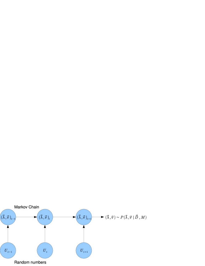
Figure 2: Scheme for producing a Markov Chain with stationary distribution $P(\vec{\lambda},\vec{\nu}|\vec{D},M)$. Independent, identically distributed random numbers are used to create random numbers, or vectors of numbers, according to any desired distribution.

Markov Chains are sequences of random numbers (or vectors of numbers), $X_{t}$, which have a well-defined limiting distribution, $\pi(x)$. The fundamental property of a Markov Chain is that the probability distribution for the next element in the sequence, $X_{t+1}$, depends only on the current state, and not on any previous history. A Markov Chain is completely defined by the one-step probability transition matrix, $P(X_{t+1}=y|X_{t}=x)$. Under certain conditions (recurrence, irreducibility, aperiodicity), it can be proven that the chain is ergodic; i.e., that the limiting probability to be in a given state does not depend on the starting point of the chain. The probability to be in a given state is then stationary. An MCMC is a method producing an ergodic Markov Chain which stationary distribution is the distribution of interest. In our case, we produce a Markov Chain where the stationary probability density is the desired posterior pdf; i.e., $\pi=P(\vec{\lambda},\vec{\nu}|\vec{D},M)$. A graphical description is given in Fig. 2.

The original and most popular algorithm which achieves this is the Metropolis algorithm [5].

5.2 Metropolis Algorithm

The algorithm works as follows:

1. Given that the system is in state $X_{t}=\vec{x}$, a new proposed state, $\vec{y}$, is generated according to a symmetric proposal function, $g(\vec{y},\vec{x})$. In our application, a state is a particular set of parameter values.

2. The quantity

   $$r=\frac{\pi(\vec{y})}{\pi(\vec{x})}$$

   is then calculated, and compared to a random number $U$, generated flat between $[0,1]$. If $U<r$, then we set $X_{t+1}=\vec{y}$, else, we take $X_{t+1}=\vec{x}$.

It is possible to show that, given a reasonable proposal function $g$, this algorithm satisfies the conditions of an MCMC, and that the limiting distribution is $\pi(\vec{x})$. This then allows for the production of states distributed according to the desired distribution. In particular, this allows for the generation of randomly distributed system states according to complicated probability density functions which have no analytic form. All that is required is that $\pi(\vec{x})$ can somehow be calculated.

6 Implementation

The requirements for a technical implementation of the Bayesian inference described above are (i) a flexible framework which allows to formulate the models developed, and (ii) a reliable and fast code for numerical operations such as optimization, marginalization and integration. The BAT software framework was designed to fulfill both requirements. Its technical implementation is described in the following.

6.1 Framework

The BAT software framework is C++ based code which comes in the form of a library. It offers classes which are used to phrase the problems encountered and to perform numerical operations. The framework is interfaced to software packages such as ROOT [6], Minuit [7], or the CUBA library [8]. It offers several output formats, e.g., plain ASCII files, ROOT trees and graphical displays. The BAT library can be linked against in a standalone program or be loaded into ROOT.

The formulation of models and their corresponding terms, as, e.g., in Eq. (12), is done in the form of methods which belong to the above mentioned classes. These are defined by the user. For simple applications such as fitting a histogram or a function with Poissonian or Gaussian uncertainties, the BAT software provides predefined classes which can be used with minimal programming effort.

A detailed description of the class structure and the methods is given in [9].

6.2 Numerical Implementation

The numerical operations which need to be performed during the analysis are optimization, marginalization and integration. Several algorithms for each operation are either implemented in the current version of the code or planned for later versions. Emphasis is placed on the MCMC.

MCMC

The posterior probability density of Eq. (15) is sampled using an MCMC. A pre-run of the MCMC is performed before the sampling and analysis run in order to ensure convergence and to find reasonable run parameters.

For the pre-run, several chains are run in parallel with random starting points in the allowed range. The steps in parameter space are done consecutively for each parameter and chain. The proposal function for new steps is chosen flat by default with a range initially set to the width of the allowed range of the parameter. An iteration is defined as the set of steps from an update of the first parameter of the first chain to the last parameter of the last chain. The efficiency for accepting or rejecting new points is evaluated separately for each parameter and chain over several iterations (default: $1,000$). The proposal function ranges are updated every $1,000$ iterations until an efficiency between 10% and 50% is found for each parameter. The convergence of Markov chains is monitored via the $r$-value [10], which is defined as $r=\sqrt{\hat{V}/W}$, where $\hat{V}$ is the estimated variance of the target distribution and $W$ is the mean of variances of all chains. The quantities are defined as follows:

$$W = \frac{1}{m}\frac{1}{n-1}\sum_{j=1}^{m}\sum_{i=1}^{n}(x_{i}-\bar{x}_{j})^{2}\,,$$

$$\hat{V} = (1-\frac{1}{n})W+\frac{1}{m-1}\sum_{j=1}^{m}(\bar{x}_{j}-\bar{x})^{2}\,,$$

where $m$ is the number of chains run simultaneously (default: 5), $n$ is the number of elements in one chain for which the variance is estimated (default: $1,000$ iterations), and $x$ is a quantity of interest.

Once convergence is reached both $\hat{V}$ and $W$ should be the same, i.e., $r\approx 1$. The convergence criterion is set by default to $(r-1)<0.1$ has to be fulfilled for all parameters simultaneously, as well as by the posterior pdf. The pre-run is performed for a minimum number of iterations (default: $500$) and is continued either until the chains converged and the efficiency of each parameter is found in the required range, or until a maximum number of iterations is reached (default: $1,000,000$). No output is produced during the pre-run.

The sampling and analysis run is performed for a defined number of iterations (default: $100,000$) with run parameters found in the pre-run. Several operations are performed during the sampling: the global mode is compared to the current point, histograms are filled for the marginalized distributions (Eq. (16)), and, if applicable, the probability distribution for the function being fitted to the data is evaluated. A user interface allows to perform further operations during the sampling such as evaluating arbitrary functions of the parameters.

Optimization

The BAT package extracts the mode as a standard output. In case this is the only information from the posterior pdf of interest, an interface to the ROOT version of Minuit can be used. All necessary information, such as the ranges of the parameters and the function itself, are automatically transfered to Minuit. The Minuit run parameters can be adjusted by the user.

Integration

For model comparisons via the posterior probability of the models the denominator of Eq. (22) has to be evaluated. If no analytical expression is provided by the user, a numerical integration over the posterior probability is performed. In the current version the implemented algorithms are sampled mean with and without importance sampling. Interfaces to tools such as the CUBA library are available.

Evaluation of the validity of a model

The validity of a model can be evaluated with the prescription given in section 3. In cases where the likelihood is the product of a finite number of simple expressions, BAT can generate ensemble data sets with the parameters which maximize the posterior pdf. Subsequently, the likelihood is calculated for those data sets and the $p$-value is estimated. In case the likelihood is more complicated, an external generator has to be used. The ensemble data sets can be read into BAT and used for the analysis.

For the cases where the likelihood is a product of Gaussian or Poissonian distributions, a fast evaluation of the $p$-value is possible in BAT.

6.3 Output

BAT provides the following output by default:

• a plain ASCII file which summarizes the models and their parameters. It displays the results of the analysis such as the global mode, the mean and modes of the marginalized distributions, or the uncertainties on the parameters;

• ROOT trees which store the summary information. The information of several runs with, e.g., different data sets can be stored and compared;

• ROOT trees containing the Markov Chains. All points of the chains can be stored together with an index and the posterior pdf at that point. This allows the chains to be analyzed offline;

• histograms of the marginalized distributions (1D) and histograms containing the correlation between two parameters (2D). These are stored in the form of ROOT histograms.

7 Examples

As examples of the use of BAT, we consider the analysis of two similar data sets generated using the same functional form. In the first case, the data fluctuations are taken to be Gaussian while in the second case the fluctuations are generated using a Poisson distribution. The same models are used to fit to the data in each case, but the conclusions are quite different, driven in large part by the different uncertainties assigned to the data points. We first discuss the Gaussian fitting example in some length, describing the fits and the standard BAT output. The wealth of information which can be extracted from the Markov Chain is apparent already in these simple examples. A comparison of the use of the $p$-value proposed in this paper with the posterior probability of the models is also discussed.

7.1 Example: Gaussian Uncertainties

The data shown in Fig. 3 were fitted by several models. The data point $y_{i}$ at a given $x_{i}$ was generated by sampling from a Gaussian distribution with mean $f(x_{i})$ and fixed standard deviation of $s=4$ units, where

$$f(x_{i})=A+B\,x_{i}+C\,x_{i}^{2}+\frac{D}{\sigma\sqrt{2\pi}}e^{-\frac{(x_{i}-\mu)^{2}}{2\sigma^{2}}}\,,$$ (26)

and ($A=0$, $B=0.5$, $C=0.02$, $D=15$, $\sigma=0.5$, $\mu=5.0$). The data are plotted in the usual way, with the bar on each data point indicating the size of the data uncertainty (in this case the value used to generate the data).

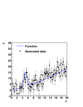
Figure 3: The data set used in the example fits described in the text. The function from which the data points were generated is shown as a dashed blue line.

The data were fitted using the following models:

1. second order polynomial;

2. constant plus Gaussian;

3. linear plus Gaussian;

4. quadratic plus Gaussian.

The likelihood function was taken to be

$$P(\vec{D}|\vec{\lambda},M)=\prod_{i}\frac{1}{\sqrt{2\pi}s}e^{-\frac{(y_{i}-f(x_{i}))^{2}}{2s^{2}}}\,,$$

where $f(x_{i})$ is evaluated using the current values of the parameters $\vec{\lambda}$ in the model. Table 1 summarizes the parameters available in each model and the range over which they are allowed to vary. In all models, flat priors were assumed for all parameters. An example with non-flat priors is discussed in a later section.

	Model	Par	Min	Max	Global	Mean/	Central $68\%$	$p$-value
					mode	Limit (95%)	interval
I.	$A_{\rm I}+B_{\rm I}\,x_{i}+C_{\rm I}\,x_{i}^{2}$	$A_{\rm I}$	-0.0	$\phantom{00}5.0$	$0.5\cdot 10^{-3}$	$<1.7$	-	$0.154$
		$B_{\rm I}$	-0.0	001.2	000.77	000.65	000.48–000.81
		$C_{\rm I}$	-0.1	000.1	$9.4\cdot 10^{-3}$	$14.6\cdot 10^{-3}$	$(5.1-24.1)\cdot 10^{-3}$
II.	$A_{\rm II}+\frac{D_{\rm II}}{\sigma_{\rm II}\,\sqrt{2\pi}}e^{-\frac{(x_{i}-\mu_{\rm II})^{2}}{2\sigma_{\rm II}^{2}}}$	$A_{\rm II}$	-0.0	010.0	003.50	003.60	003.00–004.20	0.025
		$D_{\rm II}$	-0.0	200.0	142.90	136.80	125.60–147.90
		$\mu_{\rm II}$	-2.0	018.0	017.20	017.10	016.70–017.50
		$\sigma_{\rm II}$	-0.2	004.00	004.000	$>3.5$	-
III.	$A_{\rm III}+B_{\rm III}\,x_{i}$	$A_{\rm III}$	-0.0	010.0	$0.6\cdot 10^{-3}$	$<1.5$	-	0.479
	$+\frac{D_{\rm III}}{\sigma_{\rm III}\,\sqrt{2\pi}}e^{-\frac{(x_{i}-\mu_{\rm III})^{2}}{2\sigma_{\rm III}^{2}}}$	$B_{\rm III}$	-0.0	002.0	000.89	000.77	000.63 – 000.89
		$D_{\rm III}$	-0.0	200.0	009.80	023.60	006.60 – 004.60
		$\mu_{\rm III}$	-2.0	018.0	005.20	011.90	005.10 – 017.20
		$\sigma_{\rm III}$	-0.2	004.00	000.50	002.10	000.50 – 003.60
IV.	$A_{\rm IV}+B_{\rm IV}\,x_{i}+C_{\rm IV}\,x_{i}^{2}$	$A_{\rm IV}$	-0.0	010.0	$3.6\cdot 10^{-3}$	$<1.4$	-	0.667
	$+\frac{D_{\rm IV}}{\sigma_{\rm IV}\,\sqrt{2\pi}}e^{-\frac{(x_{i}-\mu_{\rm IV})^{2}}{2\sigma_{\rm IV}^{2}}}$	$B_{\rm IV}$	-0.0	002.0	000.51	000.42	000.26–005.84
		$C_{\rm IV}$	-0.0	000.5	$25.4\cdot 10^{-3}$	$28.1\cdot 10^{-3}$	$(18.1-3.8)\cdot 10^{-3}$
		$D_{\rm IV}$	-0.0	200.0	012.56	012.80	008.90 – 016.30
		$\mu_{\rm IV}$	-2.0	018.0	005.20	005.50	004.90 – 005.40
		$\sigma_{\rm IV}$	-0.2	004.0	000.55	000.75	000.48 – 000.87

Table 1: Summary of the models fitted to the data, along with the ranges allowed for the parameters. The value of the parameter from the global mode, the mean (or $95$% probability limit for a parameter if it is at the edge of the allowed range) and the central $68$% probability interval from the marginalized distribution are given. The last column gives the $p$-value of the fit.

The fits themselves are shown in Fig. 4, while the results for the mode, the mean and the central 68% intervals on the parameters are given in Tab. 1. The solid lines in Fig. 4 are the functional forms evaluated with the parameters set to the global mode values. For the calculation of the uncertainty band, the output of the Markov Chain was used to produce a distribution of $y$-values from the model at different $x$-values. The central 68% probability interval of these $y$-values then defines the uncertainty band. We note the following:

• the fit functions all give a reasonable description of the data within the constraints allowed by the functional forms;

• the values of the functions evaluated at the parameter values from the global mode can lie outside the central probability interval (e.g., the peak region in model III).

The possibility of having multiple modes in the probability distributions as well as a different definition of the uncertainty interval will be discussed later.

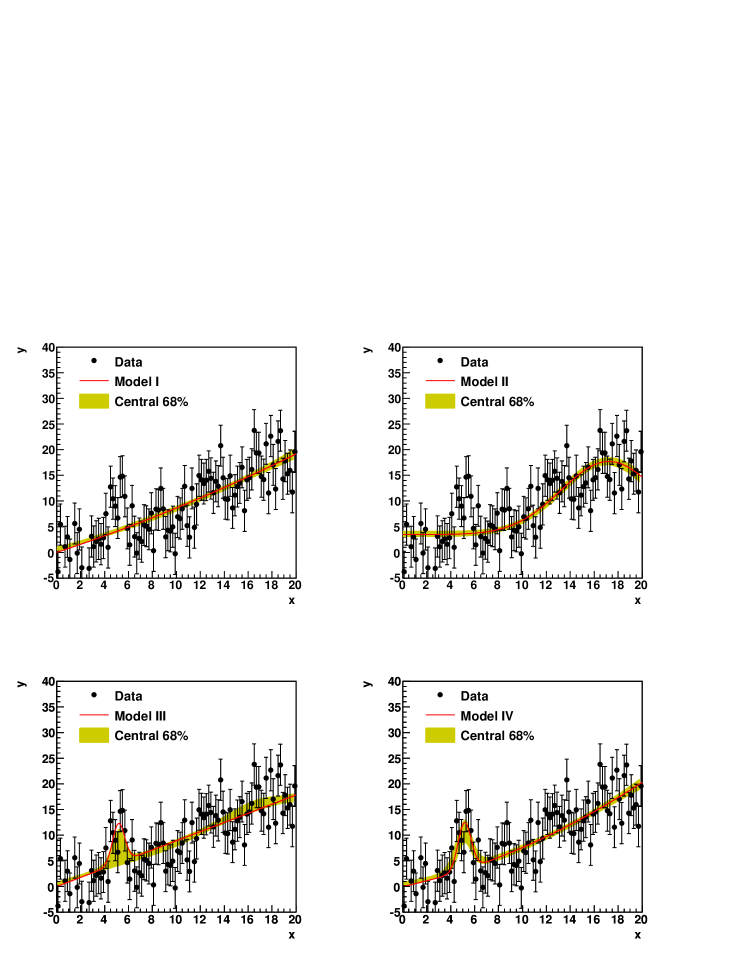
Figure 4: Graphical display of the model fits to the data. The solid lines give the models with the parameters set to the global mode values. The band is calculated as explained in the text.

7.1.1 The Posterior pdf

The BAT program outputs a file containing sets of parameter values distributed according to the full posterior pdf. In addition, the BAT program produces graphical output of the marginalized posterior pdfs of all parameters and parameter pairs. The posterior pdfs of the parameters for model I are shown in Fig. 5 as an example of these marginalized distributions. For the one dimensional distributions, the dashed line marks the median. The mean and global mode are marked by the diamond and the triangle, respectively. The band gives the central $68$% probability interval. If the marginalized mode for a parameter is at one of the limits, the $95$% probability lowest or highest interval is shown instead. The median is given at the top of each plot along with the range allowed from the central $68$% probability interval. In the case where a limit is reported, the upper or lower $95$% probability value is quoted. For the two dimensional distribution the pdf is represented by a color code and the open circle marks the global mode.

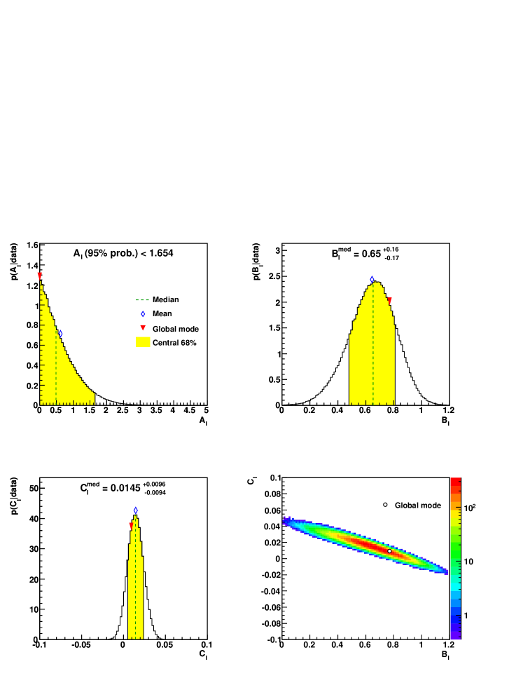
Figure 5: Examples of standard output distributions from the BAT program. The marginalized pdfs for each of the parameters from model I are shown as well as the probability contours from $P(B_{\rm I},C_{\rm I}|\vec{D})$. Note the log-scale in the bottom right plot.

7.1.2 Multiple Modes

It is often the case that there are several modes in the posterior pdf. As an example, we look in more detail at the posterior pdfs for model III. Figure 6 shows the marginalized pdfs for the amplitude, $D_{\rm III}$, and the mean of the Gaussian peak, $\mu_{\rm III}$, and the two-dimensional probability contours for the amplitude and mean, and the mean and width of the Gaussian, $\sigma_{\rm III}$. As becomes clear from these plots, it is possible for a large fraction of the probability distribution to be far from the parameter value of the global mode. The global mode can in fact lie outside the central 68% probability interval. In the fit of model III to our simulated data, two regions for the parameter $\mu_{\rm III}$ have significant probability. In one case, a low lying peak is located at $\mu_{\rm III}\approx 5$, while in the second case there is a peak located at $\mu_{\rm III}\approx 17$ (see Fig. 6 upper right). The peak at $\mu_{\rm III}\approx 5$ corresponds to a narrow Gaussian with small amplitude as can be seen in the lower left and lower right plot of Fig. 6. The peak at $\mu_{\rm III}\approx 17$ is broad and has a larger amplitude. The 2D-projections of the posterior pdf indicate that there are several regions with significant probability.

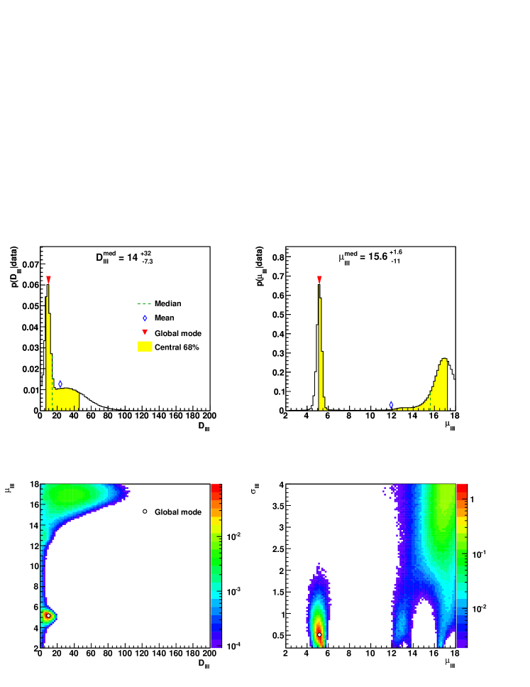
Figure 6: The marginalized pdfs for some of the parameters from model III. See text for discussion.

With BAT the level of information available allows the user to see effects such as the multiple modes clearly, and to then react accordingly. In the example discussed here, the user may want to redefine the prior ruling out the possibility of the wide Gaussian and perform the fit again.

7.1.3 Definition of Uncertainty Interval

The central interval is not always the appropriate choice for the definition of the uncertainty interval. Another option is to take the narrowest set of intervals containing $68$% of the posterior pdf. Choosing this definition can produce discontinuous regions in the parameter space as shown in Fig. 7. The uncertainty band on the value of the fit function at a given value of $x$ can also be calculated with this approach. As an example, Fig. 8 (left) shows the distribution of possible $y$-values for $x=5.0$. The shaded area is the smallest set of intervals containing $68$% probability. The resulting uncertainty band is shown in Fig. 8 (right).

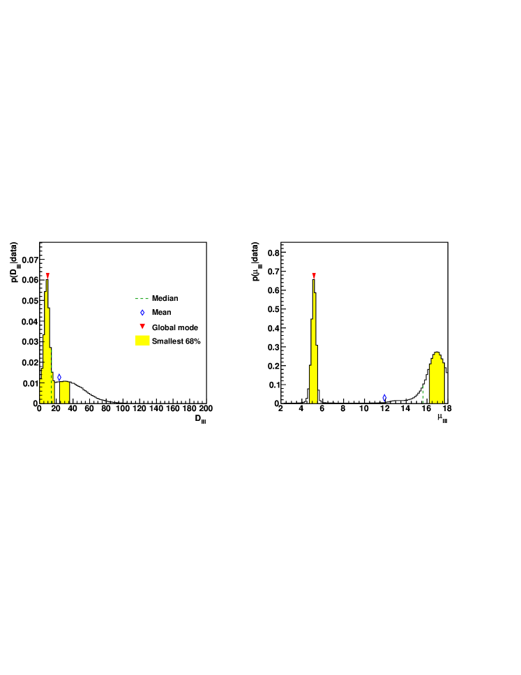
Figure 7: The marginalized pdfs for parameters $D_{\rm III}$ and $\mu_{\rm III}$ from model III using the smallest set of intervals containing $68$% of the probability.

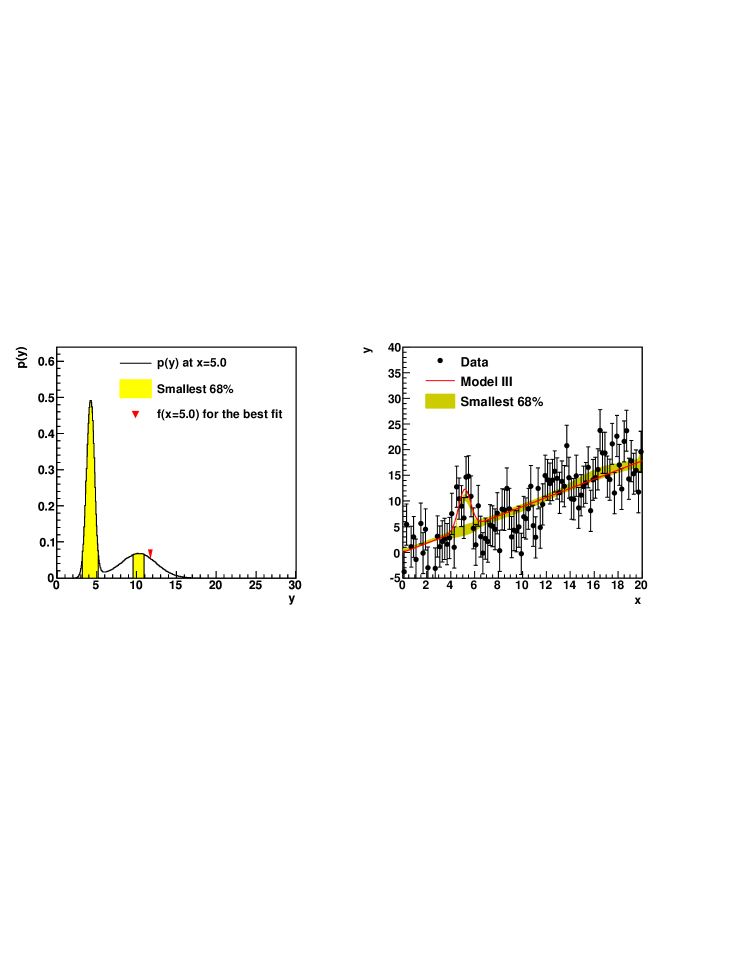
Figure 8: Results from fits of model III to the data. Left: An example for the distribution of $y$-values for a fixed value of $x=5.0$. The shaded area is the smallest set of intervals containing 68% of the probability. Right: The uncertainty band calculated using this definition.

7.1.4 Model Comparison

The model comparison can be carried out via the $p$-values given in Tab. 1. The corresponding $p$-values for models I–IV are 0.154, 0.025, 0.479 and 0.667, respectively. From the $p$-values, one concludes that models I, III and IV are all in good agreement with the data, whereas model II is somewhat disfavored. This is consistent with the conclusions one would draw from a visual inspection of the plots in Fig. 4. For this example, the $p$-value provides a useful goodness-of-fit number summarizing the ability of a model to represent the data.

It is also possible to calculate directly a posterior probability for each model to be correct. In this case, the prior probabilities for each model were taken to be the same. The posterior probabilities are then calculated according to Eq. (22). The results for the four models were $0.88$, $7.6\cdot 10^{-6}$, $0.12$ and $8.2\cdot 10^{-3}$, respectively. These values are very sensitive to the range allowed for the parameter values in the model, and models with more parameters are automatically disfavored. Making use of this probability requires a very considered choice of the priors used for the models as well as the priors on the individual parameters within a model.

7.2 Example: Poissonian Uncertainties

In this example, the data were generated assuming the expression in Eq. (26) is the expectation value for a Poisson distribution in bin $i$. I.e., the number of events in the $i$th bin, $n_{i}$, was simulated using a Poisson distributed number with mean $f(x_{i})$. The same models were fitted to the data, and the parameter ranges were those specified in Tab. 1. The data which were fitted are shown in Fig. 9, together with the models evaluated using the parameter values from the global mode of the fits.

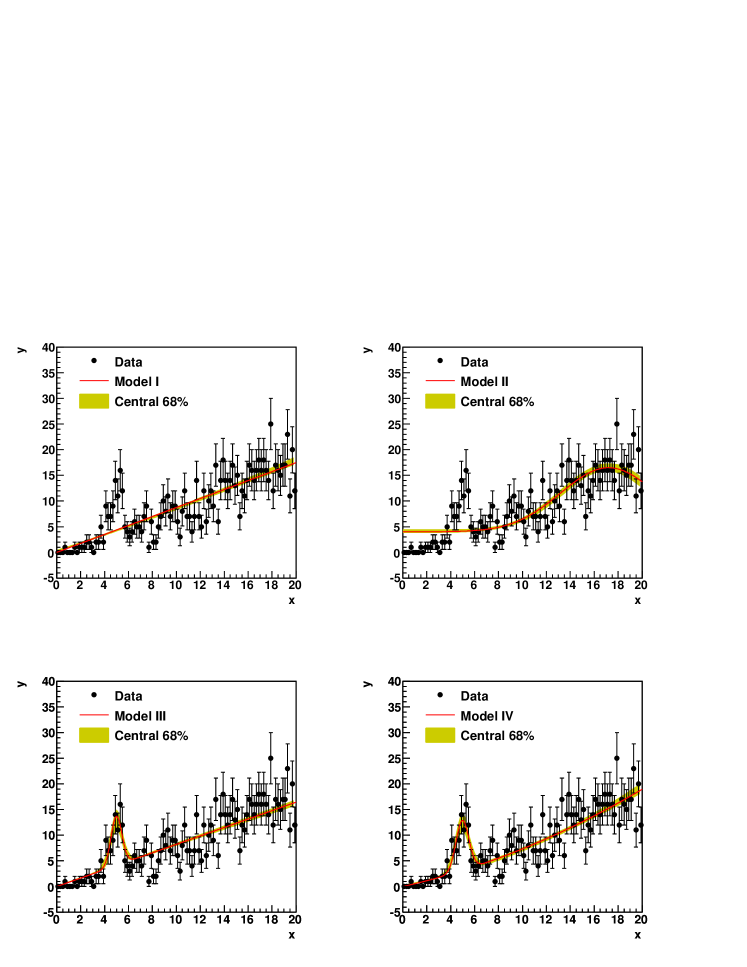
Figure 9: The data set as well as the fitted functions for the example with Poissonian fluctuations. Upper left, model I; upper right, model II; lower left, model III; lower right, model IV. The shaded band shows the uncertainty on the fit functions from the central 68% interval.

This example represents a typical histogram fitting application. The data in bins represent the result of a counting experiment, and the likelihood function is

$$P(\vec{D}|\vec{\lambda},M)=\prod_{i}\frac{e^{-f(x_{i})}\,f(x_{i})^{n_{i}}}{n_{i}!}\,,$$

where $f(x_{i})$ is the prediction for the mean for bin $i$ for a given model, $M$.

In this case, we find that the models are easily distinguished. There is a much stronger discrimination between the models since the uncertainties on the data are considerably smaller. The distribution of $f^{*}$ (see Eq. (18)) for $10^{6}$ simulated experiments for each of the models is shown in Fig. 10, along with the value of $f^{D}$. The resulting $p$-values are $0.3\cdot 10^{-3}$, $<3\cdot 10^{-6}$, $0.563$ and $0.551$ for models I–IV, respectively. The upper limit on the $p$-value for the second model results from finding $0$ simulated experiments with such a low likelihood, and corresponds to a $95$% upper limit. The models I and II can be clearly distinguished from the models III and IV. It is not possible to distinguish the latter two models based on the $p$-value, and in practice the model with fewer parameters would be preferred.

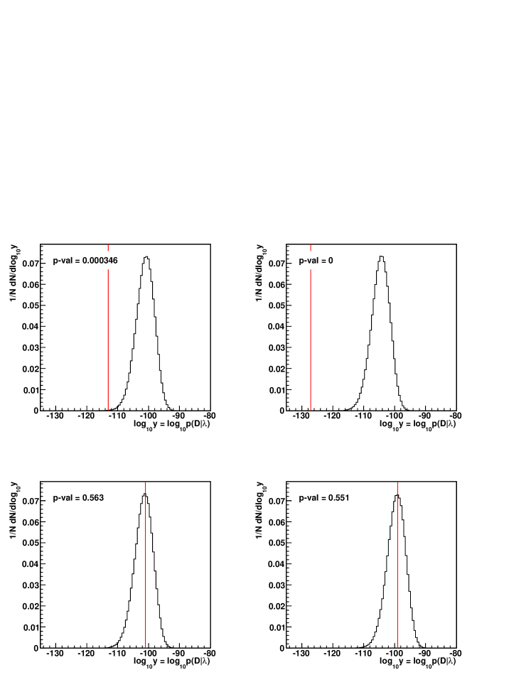
Figure 10: Distribution of $f^{*}$ for models I–IV (histogram). The value of $f^{D}$ is shown as the red vertical line. The $p$-values are calculated based on Eq. (18).

7.2.1 Non-flat priors

As an example of the influence of the prior used for an individual parameter in the extraction of the posterior pdf, a different prior was used for the parameter $\sigma$ in models II, III and IV. This restriction could come from a known detector resolution, e.g., which would limit the observed width of any bumps in the data. Rather than using a flat prior, the following form was chosen:

$$P_{0}(\sigma)=\frac{1}{0.3\sqrt{2\pi}}e^{-\frac{(\sigma-0.7)^{2}}{0.18}}\,.$$

No significant differences in the marginalized distributions and the $p$-values were found for models III and IV, since the data already constrain these quite well. However, the solution with a large value of $\sigma_{\rm II}$ in model II, discussed above, was now suppressed, and $f^{D}$ for the fit was reduced. This clearly illustrates the need to put the maximum amount of knowledge into the fitting procedure in order to get out the best possible results.

8 Summary

We have described the development of a general purpose analysis tool based on a Bayesian learning algorithm, the BAT package. BAT is based on the Markov Chain Monte Carlo technique, and provides all the standard quantities such as best fit parameters, goodness-of-fit, upper limits, etc. In addition, BAT provides a sampling of the parameters of the model under study according to the full posterior probability density function. This allows for detailed investigations of correlations between parameters, and the evaluation of the probability density for any function of the parameters, without approximations. We believe this extra functionality will be very useful in data analysis.

The BAT package is coded in C++ and is available under http://mppmu.mpg.de/bat/. A manual describing the use of BAT is also available at that location.

9 Acknowledgements

We would like to thank Giulio d’Agostini and Massimo Corradi for very enlightening discussions. Special thanks also to Andrea Knue, an early user of the BAT package, and Daniel Greenwald.

References

- [1] G. D’Agostini, Bayesian Reasoning in Data Analysis - A Critical Introduction, World Scientific, 2003.
- [2] A. Gelman, J.B. Carlin, H. S. Stern, D. B. Rubin, Bayesian Data Analysis, 2nd edition, Chapman & Hall/CRC, 2004.
- [3] A. Caldwell and K. Kröninger, Phys. Rev. D 74 (2006) 092003.
-
[4]
See, e.g.,
S. Karlin and H. Taylor, A First Course in Stochastic Processes, Academic Press, 1975;
W. R. Gilks, S. Richardson, D. Spiegelhalter (Editors), Markov Chain Monte Carlo in Practice, Chapman and Hall, 1996. - [5] N. Metropolis et al., J. Chem. Phys. 21 (1953) 1087.
- [6] R. Brun and F. Rademakers, Nucl. Instrum. Meth. A 389 (1997) 81.
- [7] F. James and M. Roos, Comput. Phys. Commun. 10 (1975) 343.
- [8] T. Hahn, Comput. Phys. Commun. 168, 78 (2005) [arXiv:hep-ph/0404043].
- [9] http://www.mppmu.mpg.de/bat/
- [10] A. Gelman and D. Rubin, Inference from iterative simulations using multiple sequences, Statistical Science 7 (1992) 457-511.