Tau sleptons and Tau sneutrino Decays in MSSM under the Cosmological Bounds

Abstract

We present the numerical investigation of the fermionic two-body decays of tau sleptons $\tilde{\tau}_{1,2}$ and $\tau$ sneutrino in the Minimal Supersymmetric Standard Model with complex parameters. In the analysis we particularly take into account the cosmological bounds imposed by WMAP data. We plot the CP-phase dependences for each fermionic two-body channel of $\tilde{\tau}_{1,2}$ and $\tau$ sneutrino and speculate about the branching ratios and total (two-body) decay widths. We find that the phase dependences of the decay widths of the third family sleptons are quite significant which can provide viable probes of additional CP sources. We also draw attention to the polarization of the final-state tau in the $\tilde{\tau}_{1,2}$ decays.
Key Words: CP-phase, sleptons decays, WMAP-allowed band.

1 Introduction

The experimental HEP frontier is soon reaching TeV energies and most of the physicists expect that just there theoretically proposed Higgs bosons and superpartners are waiting to be discovered. There are many reasons to be so optimistic. First of all, in spite of its remarkable successes, the Standard Model has to be extended into a more complete theory which should solve the hierarchy problem and stabilize the Higgs boson mass against radiative corrections. The most attractive extension to realize these objectives is supersymmetry (SUSY) [1]. Its minimal version (MSSM) requires a non-standard Higgs sector [2] which introduces additional sources of CP-violation[3, 4] beyond the $\delta_{CKM}$ phase [5]. The plethora of CP-phases also influences the decays and mixings of B mesons (as well as D and K mesons). The present experiments at BABAR, Tevatron and KEK and the one to start at the LHC will be able to measure various decay channels to determine if there are supersymmetric sources of CP violation. In particular, CP-asymmetry and decay rate of $B\rightarrow X_{s}\gamma$ form a good testing ground for low-energy supersymmetry with CP violation [6]. The above-mentioned additional CP-phases explain the cosmological baryon asymmetry of the universe and the lightest SUSY particle could be an excellent candidate for cold dark matter in the universe [7, 8].

In the case of exact supersymmetry, all scalar particles would have to have same masses with their associated SM partners. Since none of the superpartners has been discovered, supersymmetry must be broken. But in order to preserve the hierarchy problem solved the supersymmetry must be broken softly. This leads to a reasonable mass splittings between known particles and their superpartners, i.e. to the superpartners masses around 1 TeV.

The precision experiments by Wilkinson Microwave Anisotropy Probe (WMAP) [9] have put the following constraint on the relic density of cold dark matter

$$0.0945<\Omega_{CDM}h^{2}<0.1287$$ (1)

Recently, in the light of this cosmological constraint an extensive analysis of the neutralino relic density in the presence of SUSY-CP phases has been given by Bélanger et al. [10].

Analyses of the decays of third generation scalar quarks [12] and scalar leptons [13] with complex SUSY parameters have been performed by Bartl et al. In this study we present the numerical investigation of the fermionic two-body decays of third family sleptons in MSSM with complex SUSY parameters taking into account the cosmological bound imposed by WMAP data. Actually, we had performed some studies in this direction for squarks [14, 15] incorporating all the existing bounds on the SUSY parameter space by utilizing the study by Belanger et al. [10] before. These investigations showed us that the effects of $M_{1}$ and its phase $\varphi_{U(1)}$ on the decay widths of squarks are quite significant. Now we consider third generation sleptons. Namely, we study the effect of $M_{1}$ and its phase $\varphi_{U(1)}$ on the decay widths of $\tilde{\tau}_{1,2}$ and $\tilde{\nu}_{\tau}$.

In the numerical calculations, although the SUSY parameters $\mu$, $M_{1}$, $M_{2}$, and $A_{f}$ are in general complex, we assume that $\mu$, $M_{2}$ and $A_{f}$ are real, but $M_{1}$ and its phase $\varphi_{U(1)}$ take values on the WMAP- allowed bands given in Ref. [10]. These bands also satisfy the EDM bounds [16]. The experimental upper limits on the EDMs of electron, neutron and the ${}^{299}Hg$ and the ${}^{205}Tl$ atoms may impose constraints on the size of the SUSY CP-phases [17, 18]. However, these constraints are highly model dependent. This means that it is possible to suppress the EDMs without requiring the various SUSY CP-phases be small. For example, in the MSSM assuming strong cancellations between different contributions [19], the phase of $\mu$ is restricted to $|\varphi_{\mu}|<\pi/10$, but there is no such restriction on the phases of $M_{1}$ and $A_{f}$. In addition, we evaluate the parameter $M_{2}$ via the relation $M_{2}=(3/5)|M_{1}|(\tan\theta_{W})^{-2}$ which can be derived by assuming gaugino mass unification purely in the electroweak sector of MSSM. It is very important to insert the WMAP-allowed band in the plane $M_{1}-\varphi$ into the numerical calculations instead of taking one fixed $M_{1}$ value for all $\varphi$-phases, because, for example, on the allowed band for $\mu=200$ GeV, $M_{1}$ starts from 140 GeV for $\varphi=0$ and increasing monotonically it becomes 165 GeV for $\varphi=\pi$. In Ref.[10] two WMAP-allowed band plots are given, one for $\mu=200$ GeV and the other for $\mu=350$ GeV. For both plots the other parameters are fixed to be $\tan\beta=10$, $m_{H^{+}}=1$ TeV, $A_{f}=1.2$ TeV and $\varphi_{\mu}$=$\varphi_{A_{f}}$=0. We here choose the masses for $\tilde{\tau}_{1,2}$ sleptons as $m_{\tilde{\tau}_{2}}$=1000 GeV and $m_{\tilde{\tau}_{1}}$=750 GeV. These $m_{\tilde{\tau}_{1,2}}$ values lead to a sneutrino mass $m_{\tilde{\nu}_{\tau}}$=745 GeV for $M_{\tilde{L}}<M_{\tilde{E}}$.

2 Tau Sleptons and Tau Sneutrino Masses, Mixing and Decay Widths

2.1 Masses and mixing in slepton sector

The superpartners of the SM fermions with left and right helicity are the left and right sfermions. In the case of tau slepton (stau) the left and right states are in general mixed. Therefore, the sfermion mass terms of the Lagrangian are described in the basis ($\tilde{\tau}_{L}$,$\tilde{\tau}_{R}$) as [20, 21]

$${\cal L}_{M}^{\tilde{\tau}}=-({\tilde{\tau}}_{L}^{{\dagger}}{\tilde{\tau}}_{R}^{{\dagger}})\left(\begin{array}[]{cc}M_{LL}^{2}&M_{LR}^{2}\\[4.30554pt] M_{RL}^{2}&M_{RR}^{2}\end{array}\right)\left(\begin{array}[]{c}\tilde{\tau}_{L}\\[4.30554pt] \tilde{\tau}_{R}\end{array}\right)$$ (2)

with

$$M_{LL}^{2} = M_{\tilde{L}}^{2}+(I_{3L}^{\tau}-e_{\tau}\sin^{2}\theta_{W})\cos(2\beta)m_{z}^{2}+m_{\tau}^{2},$$ (3)

$$M_{RR}^{2} = M_{\tilde{E}}^{2}+e_{\tau}\sin^{2}\theta_{W}\cos(2\beta)m_{z}^{2}+m_{\tau}^{2},$$ (4)

$$M_{RL}^{2} = (M_{LR}^{2})^{*}=m_{\tau}(A_{\tau}-\mu^{*}(\tan\beta)^{-2I_{3L}^{\tau}}),$$ (5)

where $m_{\tau}$, $e_{\tau}$, $I_{3L}^{\tau}$ and $\theta_{W}$ are the mass, electric charge, weak isospin of the $\tau$-lepton and the weak mixing angle, respectively. $\tan\beta=v_{2}/v_{1}$ with $v_{i}$ being the vacuum expectation values of the Higgs fields $H_{i}^{0}$, $i=1,2$. The soft SUSY-breaking parameters $M_{\tilde{L}}$, $M_{\tilde{E}}$ and $A_{\tau}$ involved in Eqs. (3-5) can be evaluated for our numerical calculations using the following relations:

$$M_{\tilde{L}}^{2} = \frac{1}{2}{\left(m_{\tilde{\tau}_{1}}^{2}+m_{\tilde{\tau}_{2}}^{2}\pm\sqrt{(m_{\tilde{\tau}_{2}}^{2}-m_{\tilde{\tau}_{1}}^{2})^{2}-4m_{\tau}^{2}|A_{\tau}-\mu^{*}\cot\beta|^{2}}\right)}$$ (6)

$$+(\frac{1}{2}-\sin^{2}\theta_{W})\cos(2\beta)m_{z}^{2}-m_{\tau}^{2},$$

$$M_{\tilde{E}}^{2} = \frac{1}{2}{\left(m_{\tilde{\tau}_{1}}^{2}+m_{\tilde{\tau}_{2}}^{2}\mp\sqrt{(m_{\tilde{\tau}_{2}}^{2}-m_{\tilde{\tau}_{1}}^{2})^{2}-4m_{\tau}^{2}|A_{\tau}-\mu^{*}\cot\beta|^{2}}\right)}$$ (7)

$$+\sin^{2}\theta_{W}\cos(2\beta)m_{z}^{2}-m_{\tau}^{2}$$

The $\tilde{\tau}$ mass eigenstates $\tilde{\tau}_{1}$ and $\tilde{\tau}_{2}$ can be obtained from the weak states $\tilde{\tau}_{L}$ and $\tilde{\tau}_{R}$ via the $\tilde{\tau}$-mixing matrix

$${\cal R}^{\tilde{\tau}}=\left(\begin{array}[]{cc}e^{i\varphi_{\tilde{\tau}}}\cos\theta_{\tilde{\tau}}&\sin\theta_{\tilde{\tau}}\\[4.30554pt] -\sin\theta_{\tilde{\tau}}&e^{-i\varphi_{\tilde{\tau}}}\cos\theta_{\tilde{\tau}}\end{array}\right)$$ (8)

where

$$\varphi_{\tilde{\tau}}=\arg[M_{RL}^{2}]=\arg[A_{\tau}-\mu^{*}(\tan\beta)^{-2I_{3L}^{\tau}}]$$ (9)

and

$$\cos\theta_{\tilde{\tau}}=\frac{-|M_{LR}^{2}|}{\sqrt{|M_{LR}^{2}|^{2}+(m_{\tilde{\tau}_{1}}^{2}-M_{LL}^{2})^{2}}},\qquad\sin\theta_{\tilde{\tau}}=\frac{M_{LL}^{2}-m_{\tilde{\tau}_{1}}^{2}}{\sqrt{|M_{LR}^{2}|^{2}+(m_{\tilde{\tau}_{1}}^{2}-M_{LL}^{2})^{2}}}$$ (10)

One can easily get the following stau mass eigenvalues by diagonalizing the mass matrix in Eq. (2):

$$m_{\tilde{\tau}_{1,2}}^{2}=\frac{1}{2}{\left(M_{LL}^{2}+M_{RR}^{2}\mp\sqrt{(M_{LL}^{2}-M_{RR}^{2})^{2}+4|M_{LR}^{2}|^{2}}\right)},\qquad m_{\tilde{\tau}_{1}}<m_{\tilde{\tau}_{2}}$$ (11)

The $\tilde{\nu}_{\tau}$ appears only in the left state. Its mass is given by

$$m_{\tilde{\nu}_{\tau}}^{2}=M_{\tilde{L}}^{2}+\frac{1}{2}\cos(2\beta)m_{z}^{2}$$ (12)

Note that in this work we neglect CP-violation effects related to flavor change. Besides that the scalar mass matrices and trilinear scalar coupling parameters are assumed to be flavor diagonal.

2.2 Fermionic decay widths of $\tilde{\tau}_{i}$ and $\tilde{\nu}_{\tau}$

The lepton-slepton-chargino and lepton-slepton-neutralino Lagrangians have been first given in Ref. 1. Here we use them in notations of Ref. 13:

$${\cal L}_{l^{\prime}\tilde{l}\tilde{\chi}^{\pm}}=g\bar{u}(\ell_{ij}^{\tilde{d}}P_{R}+k_{ij}^{\tilde{d}}P_{L}){\tilde{\chi}}_{j}^{+}{\tilde{d}}_{i}+g\bar{d}(\ell_{ij}^{\tilde{u}}P_{R}+k_{ij}^{\tilde{u}}P_{L}){\tilde{\chi}}_{j}^{+c}{\tilde{u}}_{i}+h.c.$$ (13)

and

$${\cal L}_{l\tilde{l}\tilde{\chi}^{0}}=g\bar{l}(a_{ij}^{\tilde{l}}P_{R}+b_{ij}^{\tilde{l}}P_{L}){\tilde{\chi}}_{j}^{0}{\tilde{l}}_{i}+h.c.$$ (14)

where u ($\tilde{u}$) stands for (s)neutrinos and d ($\tilde{d}$) stands for charged (s)leptons. We also borrow the formulas for the partial decay widths of $\tilde{l}_{i}$ ($\tilde{l}_{i}$ = $\tilde{\tau}_{i}$ and $\tilde{\nu}_{\tau}$) into lepton-neutralino (or chargino) from Ref. 13. The partial decay width for the decay $\tilde{\tau}_{i}\rightarrow\tilde{\chi}_{j}^{0}+\tau(\lambda_{\tau})$ is expressed as

$$\Gamma(\tilde{\tau}_{i}\rightarrow\tilde{\chi}_{j}^{0}+\tau(\lambda_{\tau})) = \frac{g^{2}\kappa^{1/2}(m_{\tilde{\tau}_{i}}^{2},m_{\tilde{\chi}_{j}^{0}}^{2},m_{\tau}^{2})}{16\pi m_{\tilde{\tau}_{i}}^{3}}|\mathcal{M}_{\lambda_{\tau}}|^{2}$$ (15)

with

$$|\mathcal{M}_{\lambda_{\tau}}|^{2} = \frac{1}{4}\{H_{s}^{2}[|b_{ij}^{\tilde{\tau}}|^{2}+|a_{ij}^{\tilde{\tau}}|^{2}+2Re(b_{ij}^{\tilde{\tau}*}a_{ij}^{\tilde{\tau}})]$$ (16)

$$+H_{p}^{2}[|b_{ij}^{\tilde{\tau}}|^{2}+|a_{ij}^{\tilde{\tau}}|^{2}-2Re(b_{ij}^{\tilde{\tau}*}a_{ij}^{\tilde{\tau}})]$$

$$+2(-1)^{\lambda_{\tau}+(1/2)}H_{p}H_{s}(|a_{ij}^{\tilde{\tau}}|^{2}-|b_{ij}^{\tilde{\tau}}|^{2})\}$$

where $\lambda_{\tau}=\pm\frac{1}{2}$ is the helicity of the outgoing $\tau$, $\kappa(x,y,z)=x^{2}+y^{2}+z^{2}-2(xy+xz+yz)$, $H_{s}=[m_{\tilde{\tau}_{i}}^{2}-(m_{\tilde{\chi}_{j}^{0}}+m_{\tau})^{2}]^{1/2}$ and $H_{p}=[m_{\tilde{\tau}_{i}}^{2}-(m_{\tilde{\chi}_{j}^{0}}-m_{\tau})^{2}]^{1/2}$.

The explicit forms of the couplings, $a_{ij}^{\tilde{\tau}}$, $b_{ij}^{\tilde{\tau}}$ and $\ell_{ij}^{\tilde{\tau}}$, are

$$a_{ij}^{\tilde{\tau}}={\cal R}_{in}^{{\tilde{\tau}}^{*}}{\cal A}_{jn}^{\tau},\qquad b_{ij}^{\tilde{\tau}}={\cal R}_{in}^{{\tilde{\tau}}^{*}}{\cal B}_{jn}^{\tau},\qquad\ell_{ij}^{\tilde{\tau}}={\cal R}_{in}^{{\tilde{\tau}}^{*}}{\cal O}_{jn}^{\tau}\qquad(n=L,R)$$ (17)

where

$${\cal A}_{j}^{\tau}=\begin{pmatrix}\ f_{Lj}^{\tau}\\ \ h_{Rj}^{\tau}\\ \end{pmatrix},\qquad{\cal B}_{j}^{\tau}=\begin{pmatrix}\ h_{Lj}^{\tau}\\ \ f_{Rj}^{\tau}\\ \end{pmatrix},\qquad{\cal O}_{j}^{\tau}=\begin{pmatrix}\ -U_{j1}\\ \ Y_{\tau}U_{j2}\\ \end{pmatrix},$$ (18)

and

$$f_{Lj}^{\tau} = -\frac{1}{\sqrt{2}}(N_{j2}+\tan\theta_{W}N_{j1})$$

$$f_{Rj}^{\tau} = \sqrt{2}\tan\theta_{W}N_{j1}^{*}$$

$$h_{Lj}^{\tau} = (h_{Rj}^{\tau})^{*}=Y_{\tau}N_{j3}^{*}.$$ (19)

The partial decay width of $\tilde{\tau}_{i}$ into the chargino, $\tilde{\tau}_{i}\rightarrow\tilde{\chi}_{j}^{-}+\nu{{}_{\tau}}$, is obtained by the replacements $a_{ij}^{\tilde{\tau}}\rightarrow\ell_{ij}^{\tilde{\tau}}$, $b_{ij}^{\tilde{\tau}}\rightarrow 0$, $m_{\tilde{\chi}_{j}^{0}}\rightarrow m_{\tilde{\chi}_{j}^{-}}$, $m_{\tau}\rightarrow 0$ and $\lambda_{\tau}\rightarrow-\frac{1}{2}$ in Eq. (15) and Eq. (16) with the couplings $\ell_{ij}^{\tilde{\tau}}$ also given in Eq. (17) and Eq. (18).

The width for the $\tau$-sneutrino decay $\tilde{\nu}_{\tau}\rightarrow{\tilde{\chi}_{j}^{0}}\nu_{\tau}$ is obtained by the replacements $a_{ij}^{\tilde{\tau}}\rightarrow a_{j}^{\tilde{\nu}}$, $b_{ij}^{\tilde{\tau}}\rightarrow 0$, $m_{\tilde{\tau}_{i}}\rightarrow m_{\tilde{\nu}_{\tau}}$, $m_{\tau}\rightarrow 0$ and $\lambda_{\tau}\rightarrow-\frac{1}{2}$ in Eq. (15) and Eq. (16), and that for the decay $\tilde{\nu}_{\tau}\rightarrow{\tilde{\chi}_{j}^{+}}\tau(\lambda_{\tau})$ by the replacements $a_{ij}^{\tilde{\tau}}\rightarrow\ell_{j}^{\tilde{\nu}}$, $b_{ij}^{\tilde{\tau}}\rightarrow k_{j}^{\tilde{\nu}}$, $m_{\tilde{\tau}_{i}}\rightarrow m_{\tilde{\nu}_{\tau}}$ and $m_{\tilde{\chi}_{j}^{0}}\rightarrow m_{\tilde{\chi}_{j}^{+}}$. The coupling are now

$$a_{j}^{\tilde{\nu}}=\frac{1}{\sqrt{2}}(\tan\theta_{W}N_{j1}-N_{j2}),\qquad k_{j}^{\tilde{\nu}}=Y_{\tau}U_{j2}^{*},\qquad\ell_{j}^{\tilde{\nu}}=-V_{j1}.$$ (20)

Here, N is the $4\times 4$ neutralino mixing matrix, U and V are $2\times 2$ chargino mixing matrices and $Y_{\tau}=m_{\tau}/(\sqrt{2}m_{W}\cos\beta)$ is the $\tau$ Yukawa coupling.

In this work we contend with tree-level amplitudes as we aim at determining the phase-sensitivities of the decay rates, mainly.

3 Tau-Slepton and Tau-Sneutrino Decays

Here we present the dependences of the $\tilde{\tau}_{1,2}$ and $\tilde{\nu}_{\tau}$ two-body decay widths on the $\varphi_{U(1)}$ for $\mu=200$ GeV and for $\mu=350$ GeV. We also choose the values for the masses ($m_{\tilde{\tau}_{1}}$, $m_{\tilde{\tau}_{2}}$, $m_{\tilde{\chi}_{1}^{\pm}}$, $m_{\tilde{\chi}_{2}^{\pm}}$, $m_{\tilde{\chi}_{1}^{0}}$) = (750 GeV, 1000 GeV, 180 GeV, 336 GeV, 150 GeV) for $\mu=200$ GeV and ($m_{\tilde{\tau}_{1}}$, $m_{\tilde{\tau}_{2}}$, $m_{\tilde{\chi}_{1}^{\pm}}$, $m_{\tilde{\chi}_{2}^{\pm}}$, $m_{\tilde{\chi}_{1}^{0}}$) = (750 GeV, 1000 GeV, 340 GeV, 680 GeV, 290 GeV) for $\mu=350$ GeV. The mass values of these $\tau$-sleptons lead to a sneutrino mass $m_{\tilde{\nu}_{\tau}}$=745 GeV. Note that although the neutralino and chargino masses vary with $\varphi_{U(1)}$, these variations are not large. Therefore, as a final state particle (i.e., on mass-shell), we have chosen fixed (average) mass values for charginos and neutralinos. For both sets of values by calculating the $M_{\tilde{L}}$ and $M_{\tilde{E}}$ values corresponding to $m_{\tilde{\tau}_{1}}$ and $m_{\tilde{\tau}_{2}}$, we plot the decay widths for $M_{\tilde{L}}\geq M_{\tilde{E}}$ and $M_{\tilde{L}}<M_{\tilde{E}}$, separately. We plot the $\varphi_{U(1)}$-dependences of the $\tilde{\nu}_{\tau}$ partial decay widths only for $M_{\tilde{L}}<M_{\tilde{E}}$. In the case of $M_{\tilde{L}}>M_{\tilde{E}}$, the phase dependences do not change, but decay widths take larger values. In our figures, we display the slepton decay widths for the both helicity states of the outgoing $\tau$ ($\tau_{L}$ and $\tau_{R}$).

$M_{\tilde{L}}>M_{\tilde{E}}$ for $\mu=200$ GeV:

In Figure 1(a) we show the partial decay widths of the channels $\tilde{\tau}_{1}\rightarrow\tilde{\chi}_{1}^{-}\nu_{\tau}$, $\tilde{\tau}_{1}\rightarrow\tilde{\chi}_{2}^{-}\nu_{\tau}$, $\tilde{\tau}_{1}\rightarrow\tilde{\chi}_{1}^{0}\tau_{L,R}$, $\tilde{\tau}_{2}\rightarrow\tilde{\chi}_{1}^{-}\nu_{\tau}$, $\tilde{\tau}_{2}\rightarrow\tilde{\chi}_{2}^{-}\nu_{\tau}$ and $\tilde{\tau}_{2}\rightarrow\tilde{\chi}_{1}^{0}\tau_{L,R}$ as a function of $\varphi_{U(1)}$ for $\mu=200$ GeV. In these plots some dependences on the $\varphi_{U(1)}$ phase are shown. In order to see these dependences more pronouncedly, we now plot two channels separately; namely $\tilde{\tau}_{1}\rightarrow\tilde{\chi}_{1}^{0}\tau_{R}$ (the variations in the cross section are not large) and $\tilde{\tau}_{2}\rightarrow\tilde{\chi}_{1}^{0}\tau_{L}$ (the variations are really large) in Figures 4(a)-(b). Here we consider the case $M_{\tilde{L}}>M_{\tilde{E}}$, where $\tilde{\tau}_{1}$ is mainly $\tilde{\tau}_{R}$-like and $\tilde{\tau}_{2}$ is mainly $\tilde{\tau}_{L}$-like (${\cal R}_{11}^{\tilde{\tau}}$=${\cal R}_{22}^{\tilde{\tau}}$$\approx$ 0). In this case, the decay processes whose initial and final state helicities are the same, $\tilde{\tau}_{2}\rightarrow\tilde{\chi}_{2}^{-}\nu_{\tau}$, $\tilde{\tau}_{2}\rightarrow\tilde{\chi}_{1}^{-}\nu_{\tau}$, $\tilde{\tau}_{2}\rightarrow\tilde{\chi}_{1}^{0}\tau_{L}$ and $\tilde{\tau}_{1}\rightarrow\tilde{\chi}_{1}^{0}\tau_{R}$, have large widths, whereas those with opposite helicities, $\tilde{\tau}_{2}\rightarrow\tilde{\chi}_{1}^{0}\tau_{R}$, $\tilde{\tau}_{1}\rightarrow\tilde{\chi}_{1}^{-}\nu_{\tau}$, $\tilde{\tau}_{1}\rightarrow\tilde{\chi}_{2}^{-}\nu_{\tau}$ and $\tilde{\tau}_{1}\rightarrow\tilde{\chi}_{1}^{0}\tau_{L}$, have small ones. The reason for these large and small widths can be traced to the couplings $a_{ij}^{\tilde{\tau}}$, $b_{ij}^{\tilde{\tau}}$, $\ell_{ij}^{\tilde{\tau}}$ and $a_{j}^{\tilde{\nu}}$, $k_{j}^{\tilde{\nu}}$, $\ell_{j}^{\tilde{\nu}}$. Because of $H_{s}$$\approx$$H_{p}$ (since $m_{\tilde{\tau}_{1,2}}$$\gg$$m_{\tau}$) we can express the decay widths of $\tilde{\tau}_{i}\rightarrow\tilde{\chi}_{j}^{0}\tau(\lambda_{\tau})$ as $\Gamma(\tilde{\tau}_{i}\rightarrow\tilde{\chi}_{j}^{0}\tau(\lambda_{\tau}=1/2))$$\propto$$|b_{ij}^{\tilde{\tau}}|^{2}$ and $\Gamma(\tilde{\tau}_{i}\rightarrow\tilde{\chi}_{j}^{0}\tau(\lambda_{\tau}=-1/2))$$\propto$$|a_{ij}^{\tilde{\tau}}|^{2}$. For example, $\Gamma(\tilde{\tau}_{1}\rightarrow\tilde{\chi}_{1}^{0}\tau_{L})$ ($\Gamma(\tilde{\tau}_{2}\rightarrow\tilde{\chi}_{1}^{0}\tau_{R})$) is suppressed because it is proportional to the term, $|a_{11}^{\tilde{\tau}}|$ $(|b_{21}^{\tilde{\tau}}|)$, which includes small Yukawa coupling ($Y_{\tau}$). On the other hand, $\Gamma(\tilde{\tau}_{1}\rightarrow\tilde{\chi}_{1}^{0}\tau_{R})$ is proportional to the square of $b_{11}^{\tilde{\tau}}$ which depends on the combination ${\cal R}_{11}^{{\tilde{\tau}}^{*}}{\cal B}_{11}^{\tau}+{\cal R}_{12}^{{\tilde{\tau}}^{*}}{\cal B}_{12}^{\tau}$ contributing largely from its second term. Similarly, since $H_{s}$=$H_{p}$, the decay widths of $\tilde{\tau}_{i}\rightarrow\tilde{\chi}_{j}^{-}+\nu{{}_{\tau}}$ can be expressed as $\Gamma(\tilde{\tau}_{i}\rightarrow\tilde{\chi}_{j}^{-}+\nu{{}_{\tau}})$$\propto$$H_{s}^{2}$$|\ell_{ij}^{\tilde{\tau}}|^{2}$. The decay widths of $\tilde{\tau}_{1}\rightarrow\tilde{\chi}_{1}^{-}\nu_{\tau}$, $\tilde{\tau}_{1}\rightarrow\tilde{\chi}_{2}^{-}\nu_{\tau}$ are also suppressed due to the very small Yukawa coupling ($\ell_{11}^{\tilde{\tau}}$$\thickapprox$$Y_{\tau}$ ${{\cal R}_{12}^{\tilde{\tau}}}^{*}U_{12}$, $\ell_{12}^{\tilde{\tau}}$$\thickapprox$$Y_{\tau}$ ${{\cal R}_{12}^{\tilde{\tau}}}^{*}U_{22}$).

Note that the decay width $\Gamma(\tilde{\tau}_{1}\rightarrow\tilde{\chi}_{1}^{0}\tau_{R})$ is 90-110 times larger than $\Gamma(\tilde{\tau}_{1}\rightarrow\tilde{\chi}_{1}^{0}\tau_{L})$ and $\Gamma(\tilde{\tau}_{2}\rightarrow\tilde{\chi}_{1}^{0}\tau_{L})$ is 10-30 times larger than $\Gamma(\tilde{\tau}_{2}\rightarrow\tilde{\chi}_{1}^{0}\tau_{R})$. From Figure 1(a) one can see that the branching ratios for $\tilde{\tau}_{2}$ are roughly $B(\tilde{\tau}_{2}\rightarrow\tilde{\chi}_{2}^{-}\nu_{\tau})$ : $B(\tilde{\tau}_{2}\rightarrow\tilde{\chi}_{1}^{0}\tau_{L})$ : $B(\tilde{\tau}_{2}\rightarrow\tilde{\chi}_{1}^{-}\nu_{\tau})$ : $B(\tilde{\tau}_{2}\rightarrow\tilde{\chi}_{1}^{0}\tau_{R})$ $\approx$ 6 : 1 : 0.5 : 0.03.

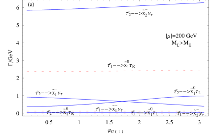
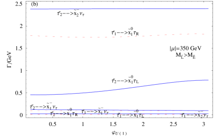
Figure 1: Partial decay widths $\Gamma$ of the $\tilde{\tau}_{1,2}$ decays for $\tan\beta=10$, $A_{\tau}=1.2$ TeV, $\varphi_{\mu}$=$\varphi_{A_{\tau}}$=0, $m_{\tilde{\tau}_{1}}=750$ GeV, $m_{\tilde{\tau}_{2}}=1000$ GeV and $M_{\tilde{L}}>M_{\tilde{E}}$; $\mu=200$ GeV in (a) and $\mu=350$ GeV in (b).

Although the $\varphi_{U(1)}$ dependence of $\Gamma(\tilde{\tau}_{2}\rightarrow\tilde{\chi}_{1}^{0}\tau_{L})$ ($\Gamma(\tilde{\tau}_{1}\rightarrow\tilde{\chi}_{1}^{0}\tau_{R})$) stems only from the parameters $|N_{11}|$ and $|N_{12}|$ ($|N_{11}|$), the phase dependence is quite pronounced. Similarly, the $\varphi_{U(1)}$ phase dependence of $\tilde{\tau}_{2}\rightarrow\tilde{\chi}_{1}^{-}(\tilde{\chi}_{2}^{-})\nu_{\tau}$ stemmed only from the $\varphi_{U(1)}$ dependence of $|U_{11}|$ ($|U_{21}|$) parameter is also quite pronounced. The decay width $\Gamma(\tilde{\tau}_{1}\rightarrow\tilde{\chi}_{1}^{0}\tau_{R})$ takes its maximum (minimum) value at $\varphi_{U(1)}$$\approx$$\frac{5\pi}{6}$ ($\varphi_{U(1)}$$\approx$$\frac{\pi}{4}$) (see Figure 4(a)). This $\varphi_{U(1)}$ value also corresponds to maximum (minimum) value of $|b_{11}^{\tilde{\tau}}|^{2}$. In a similar way, the width $\Gamma(\tilde{\tau}_{2}\rightarrow\tilde{\chi}_{1}^{0}\tau_{L})$ and its parameter $|a_{21}^{\tilde{\tau}}|^{2}$ takes their maximum (minimum) value at $\varphi_{U(1)}$$\approx$$\pi$ ($\varphi_{U(1)}$=0) (see Figure 4(b)). Hence, we can say that the phase $\varphi_{U(1)}$ dependence of $|a_{ij}^{\tilde{\tau}}|^{2}$ and $|b_{ij}^{\tilde{\tau}}|^{2}$ ($|\ell_{ij}^{\tilde{\tau}}|^{2}$) reflects the phase $\varphi_{U(1)}$ dependence of channels $\tilde{\tau}_{i}\rightarrow\tilde{\chi}_{j}^{0}\tau_{R,L}$ ($\tilde{\tau}_{i}\rightarrow\tilde{\chi}_{j}^{-}\nu_{\tau}$) directly.

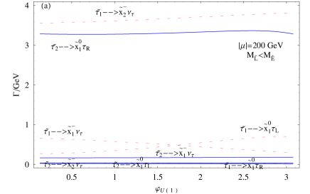
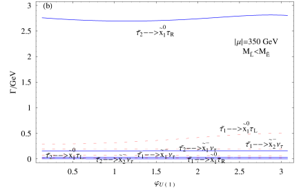
Figure 2: Partial decay widths $\Gamma$ of the $\tilde{\tau}_{1,2}$ decays for $\tan\beta=10$, $A_{\tau}=1.2$ TeV, $\varphi_{\mu}$=$\varphi_{A_{\tau}}$=0, $m_{\tilde{\tau}_{1}}=750$ GeV, $m_{\tilde{\tau}_{2}}=1000$ GeV and $M_{\tilde{L}}<M_{\tilde{E}}$; $\mu=200$ GeV in (a) and $\mu=350$ GeV in (b).

$M_{\tilde{L}}>M_{\tilde{E}}$ for $\mu=350$ GeV :

We give the same partial decay widths in Figure 1(b) for $\mu=350$ GeV (See also Figures 4(c)-(d)). Here, too, $\tilde{\tau}_{1}$ is mainly $\tilde{\tau}_{R}$-like and $\tilde{\tau}_{2}$ is mainly $\tilde{\tau}_{L}$-like because we still keep the case $M_{\tilde{L}}>M_{\tilde{E}}$. For $\mu=350$ GeV the WMAP-allowed band [10] takes place in larger $M_{1}$ values ($\sim 305-325$ GeV) leading to larger chargino and neutralino masses. This leads to smaller $H_{s}^{2}$(since $H_{s}^{2}$ $\propto$ $[m_{\tilde{\tau}_{i}}^{2}-m_{\tilde{\chi}_{j}}^{2}]$) and, as a result, smaller widths for $\tilde{\tau}_{1,2}$ decays compared with those for $\mu=200$ GeV.

As can be seen from Figure 4(d), the $\varphi_{U(1)}$ dependence of the decay $\tilde{\tau}_{2}\rightarrow\tilde{\chi}_{1}^{0}\tau_{L}$ is prominent such that the value of decay width at $\varphi_{U(1)}$=$\pi$ is about 2 times larger than that at $\varphi_{U(1)}$=$0$. The decay widths $\Gamma(\tilde{\tau}_{2}\rightarrow\tilde{\chi}_{1}^{0}\tau_{R})$, $\Gamma(\tilde{\tau}_{1}\rightarrow\tilde{\chi}_{1}^{-}\nu_{\tau})$, $\Gamma(\tilde{\tau}_{1}\rightarrow\tilde{\chi}_{2}^{-}\nu_{\tau})$ and $\Gamma(\tilde{\tau}_{1}\rightarrow\tilde{\chi}_{1}^{0}\tau_{L})$ are suppressed because of the same reasons mentioned above. The decay width of the process $\tilde{\tau}_{2}\rightarrow\tilde{\chi}_{2}^{-}\nu_{\tau}$ is the largest one among the $\tilde{\tau}_{2}$ channels and the branching ratios are $B(\tilde{\tau}_{2}\rightarrow\tilde{\chi}_{2}^{-}\nu_{\tau})$ : $B(\tilde{\tau}_{2}\rightarrow\tilde{\chi}_{1}^{0}\tau_{L})$ : $B(\tilde{\tau}_{2}\rightarrow\tilde{\chi}_{1}^{-}\nu_{\tau})$ : $B(\tilde{\tau}_{2}\rightarrow\tilde{\chi}_{1}^{0}\tau_{R})$ $\approx$ 2.4 : 0.8 : 0.1 : 0.02.

$M_{\tilde{L}}<M_{\tilde{E}}$ for $\mu=200$ GeV:

We give $\tilde{\tau}_{1,2}$ and $\tilde{\nu}_{\tau}$ decay widths as a function of $\varphi_{U(1)}$ in Figure 2(a) and Figure 3(a) respectively (for $\mu=200$ GeV). In Figures 4(e)-(f) we plot two of them separately whose CP-phase dependences are not clearly seen in Figure 2(a). They, too, show the significant dependences on CP-violation phase. In this subsection we consider the case $M_{\tilde{L}}<M_{\tilde{E}}$, where $\tilde{\tau}_{1}$ is mainly $\tilde{\tau}_{L}$-like and $\tilde{\tau}_{2}$ is mainly $\tilde{\tau}_{R}$-like (${\cal R}_{12}^{\tilde{\tau}}$=${\cal R}_{21}^{\tilde{\tau}}$$\approx$0). The decay width of the process $\tilde{\tau}_{1}\rightarrow\tilde{\chi}_{2}^{-}\nu_{\tau}$ is the largest one among the $\tilde{\tau}_{1,2}$ channels; its decay width increases from 3.55 GeV to 3.8 GeV monotonically as $\varphi_{U(1)}$ increases from 0 to $\pi$. In this case ($M_{\tilde{L}}<M_{\tilde{E}}$), the width $\Gamma(\tilde{\tau}_{1}\rightarrow\tilde{\chi}_{2}^{-}\nu_{\tau})$ is not suppressed because its $\ell_{12}^{\tilde{\tau}}$ term does not include Yukawa coupling ($\ell_{12}^{\tilde{\tau}}$$\thickapprox$ ${{\cal R}_{11}^{\tilde{\tau}}}^{*}U_{21}$). The phase dependence of $\tilde{\tau}_{2}\rightarrow\tilde{\chi}_{1}^{0}\tau_{R}$ can be seen clearly in Figure 4(f); $\Gamma(\tilde{\tau}_{2}\rightarrow\tilde{\chi}_{1}^{0}\tau_{R})$ takes its minimum and maximum values at $\varphi_{U(1)}$$\approx$$\frac{\pi}{4}$ and at $\varphi_{U(1)}$$\approx$$\frac{5\pi}{6}$ respectively, because the parameter $|b_{21}^{\tilde{\tau}}|^{2}$ reaches its minimum and maximum at these $\varphi_{U(1)}$ values.

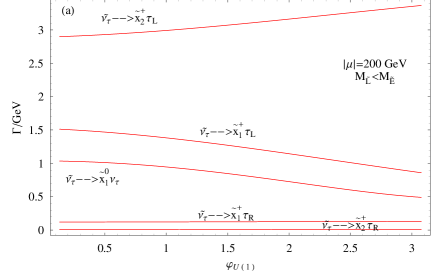
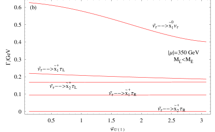
Figure 3: Partial decay widths $\Gamma$ of the $\tilde{\nu}_{\tau}$ decays for $\tan\beta=10$, $A_{\tau}=1.2$ TeV, $\varphi_{\mu}$=$\varphi_{A_{\tau}}$=0, $m_{\tilde{\tau}_{1}}=750$ GeV, $m_{\tilde{\tau}_{2}}=1000$ GeV and $m_{\tilde{\nu}_{\tau}}=745$ GeV; $\mu=200$ GeV in (a) and $\mu=350$ GeV in (b).

The branching ratios for $\tilde{\tau}_{1}$ decays are roughly $B(\tilde{\tau}_{1}\rightarrow\tilde{\chi}_{2}^{-}\nu_{\tau})$ : $B(\tilde{\tau}_{1}\rightarrow\tilde{\chi}_{1}^{0}\tau_{L})$ : $B(\tilde{\tau}_{1}\rightarrow\tilde{\chi}_{1}^{-}\nu_{\tau})$ : $B(\tilde{\tau}_{1}\rightarrow\tilde{\chi}_{1}^{0}\tau_{R})$ $\approx$ 3.8 : 0.7 : 0.3 : 0.02.

In Figure 3(a) we give $\tilde{\nu}_{\tau}$ decay widths as a function of $\varphi_{U(1)}$ for $\mu=200$ GeV. The phase dependence is more significant for the decay channels $\tilde{\nu}_{\tau}\rightarrow\tilde{\chi}_{2}^{+}\tau_{L}$, $\tilde{\nu}_{\tau}\rightarrow\tilde{\chi}_{1}^{+}\tau_{L}$ and $\tilde{\nu}_{\tau}\rightarrow\tilde{\chi}_{1}^{0}\nu_{\tau}$. Analogously to the neutralino decays of $\tilde{\tau}_{1,2}$; because of $H_{s}$$\approx$$H_{p}$ (since $m_{\tilde{\nu}_{\tau}}$$\gg$$m_{\tau}$) we can express the decay widths of $\tilde{\nu}_{\tau}\rightarrow\tilde{\chi}_{j}^{+}\tau(\lambda_{\tau})$ as $\Gamma(\tilde{\nu}_{\tau}\rightarrow\tilde{\chi}_{j}^{0}\tau(\lambda_{\tau}=1/2))$$\propto$$|k_{j}^{\tilde{\nu}}|^{2}$ and $\Gamma(\tilde{\nu}_{\tau}\rightarrow\tilde{\chi}_{j}^{0}\tau(\lambda_{\tau}=-1/2))$$\propto$$|\ell_{j}^{\tilde{\nu}}|^{2}$. To be more specific, $\Gamma(\tilde{\nu}_{\tau}\rightarrow\tilde{\chi}_{1}^{+}\tau_{R})$ ($\Gamma(\tilde{\nu}_{\tau}\rightarrow\tilde{\chi}_{2}^{+}\tau_{R})$) is suppressed because it is proportional to the term $|k_{1}^{\tilde{\nu}}|$ $(|k_{2}^{\tilde{\nu}}|)$ which includes small Yukawa coupling ($Y_{\tau}$). Since $H_{s}$=$H_{p}$ for neutrinos, the decay width of $\tilde{\nu}_{\tau}\rightarrow\tilde{\chi}_{1}^{0}+\nu_{\tau}$ can be expressed as $\Gamma(\tilde{\nu}_{\tau}\rightarrow\tilde{\chi}_{1}^{0}+\nu_{\tau})$$\propto$$H_{s}^{2}$$|a_{1}^{\tilde{\nu}}|^{2}$. The $\varphi_{U(1)}$ dependences of $\Gamma(\tilde{\nu}_{\tau}\rightarrow\tilde{\chi}_{j}^{+}\tau_{L})$ ($\Gamma(\tilde{\nu}_{\tau}\rightarrow\tilde{\chi}_{1}^{0}\nu_{\tau})$) stems from the $\varphi_{U(1)}$ dependences of $|\ell_{j}^{\tilde{\nu}}|$ ($|a_{1}^{\tilde{\nu}}|$) parameter and this parameter is quite phase-dependent.

The branching ratios for $\tilde{\nu}_{\tau}$ decays are roughly $B(\tilde{\nu}_{\tau}\rightarrow\tilde{\chi}_{2}^{+}\tau_{L})$ : $B(\tilde{\nu}_{\tau}\rightarrow\tilde{\chi}_{1}^{+}\tau_{L})$ : $B(\tilde{\nu}_{\tau}\rightarrow\tilde{\chi}_{1}^{0}\nu_{\tau})$ : $B(\tilde{\nu}_{\tau}\rightarrow\tilde{\chi}_{1}^{+}\tau_{R})$ : $B(\tilde{\nu}_{\tau}\rightarrow\tilde{\chi}_{2}^{+}\tau_{R})$ $\approx$ 3 : 1.3 : 0.1 : 0.01.

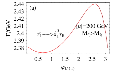
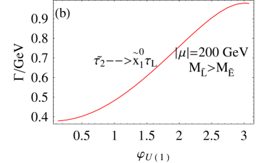
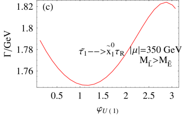
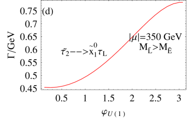
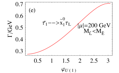
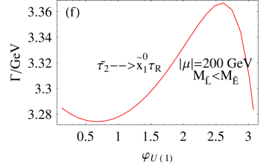
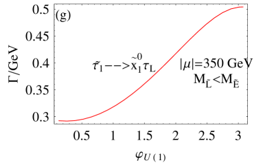
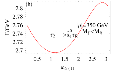
Figure 4: (a)-(h) $\varphi_{U(1)}$ dependences of certain $\tilde{\tau}_{1,2}$ decays for $\mu=200$ GeV and for $\mu=350$ GeV.

$M_{\tilde{L}}<M_{\tilde{E}}$ for $\mu=350$ GeV :

We present the dependences of the $\tilde{\tau}_{1,2}$ and $\tilde{\nu}_{\tau}$ partial decay widths on $\varphi_{U(1)}$ in Figure 2(b) and Figure 3(b) (for $\mu=350$ GeV). In this case $H_{s}^{2}$($H_{p}^{2}$) takes smaller value because of the reason mentioned in the previous subsection and this leads to smaller widths for $\tilde{\tau}_{1,2}$ and $\tilde{\nu}_{\tau}$. In Figures 4(g)-(h) we again plot two $\tilde{\tau}_{1,2}$ decay channels separately whose phase dependences are not clearly seen in Figure 2(b). The dependence of the phase $\varphi_{U(1)}$ in $\tilde{\tau}_{1,2}$ decays are similar to those in the case $M_{\tilde{L}}<M_{\tilde{E}}$ (for $\mu=200$ GeV).

Note that $\Gamma(\tilde{\tau}_{2}\rightarrow\tilde{\chi}_{1}^{0}\tau_{R})$$\approx$ 90 $\Gamma(\tilde{\tau}_{2}\rightarrow\tilde{\chi}_{1}^{0}\tau_{L})$ and $\Gamma(\tilde{\tau}_{1}\rightarrow\tilde{\chi}_{1}^{0}\tau_{L})$$\approx$ 30 $\Gamma(\tilde{\tau}_{1}\rightarrow\tilde{\chi}_{1}^{0}\tau_{R})$.

The width $\Gamma(\tilde{\nu}_{\tau}\rightarrow\tilde{\chi}_{1}^{0}+\nu_{\tau})$ decreases as the phase increases from 0 to $\pi$, showing a significant dependence on the phase. The branching ratios are roughly $B(\tilde{\nu}_{\tau}\rightarrow\tilde{\chi}_{1}^{0}\nu_{\tau})$ : $B(\tilde{\nu}_{\tau}\rightarrow\tilde{\chi}_{1}^{+}\tau_{L})$ : $B(\tilde{\nu}_{\tau}\rightarrow\tilde{\chi}_{2}^{+}\tau_{L})$ : $B(\tilde{\nu}_{\tau}\rightarrow\tilde{\chi}_{1}^{+}\tau_{R})$ : $B(\tilde{\nu}_{\tau}\rightarrow\tilde{\chi}_{2}^{+}\tau_{R})$ $\approx$ 0.6 : 0.2 : 0.15 : 0.09 : 0.0002.

4 Discussion and Summary

In this paper, we have presented the numerical investigation of the fermionic two-body decays of third family sleptons in the minimal supersymmetric standard model with complex parameters taking into account the cosmological bounds imposed by WMAP data. For this purpose, we have calculated numerically the decay widths of tau sleptons $\tilde{\tau}_{1,2}$ and $\tau$ sneutrino, paying particular attention to their dependence on the CP phase $\varphi_{U(1)}$. We have found that some decay channels like $\tilde{\tau}_{2}\rightarrow\tilde{\chi}_{2}^{-}\nu_{\tau}$, $\tilde{\tau}_{2}\rightarrow\tilde{\chi}_{1}^{-}\nu_{\tau}$, $\tilde{\tau}_{2}\rightarrow\tilde{\chi}_{1}^{0}\tau_{L}$, $\tilde{\tau}_{2}\rightarrow\tilde{\chi}_{1}^{0}\tau_{R}$, $\tilde{\tau}_{1}\rightarrow\tilde{\chi}_{2}^{-}\nu_{\tau}$, $\tilde{\tau}_{1}\rightarrow\tilde{\chi}_{1}^{-}\nu_{\tau}$, $\tilde{\tau}_{1}\rightarrow\tilde{\chi}_{1}^{0}\tau_{L}$, $\tilde{\nu}_{\tau}\rightarrow\tilde{\chi}_{2}^{+}\tau_{L}$, $\tilde{\nu}_{\tau}\rightarrow\tilde{\chi}_{1}^{+}\tau_{L}$ and $\tilde{\nu}_{\tau}\rightarrow\tilde{\chi}_{1}^{0}\nu_{\tau}$ show considerable dependences on $\varphi_{U(1)}$ phase. These decay modes will be observable at a future $\emph{e}^{+}\emph{e}^{-}$ collider and LHC. Therefore they provide viable probes of CP violation beyond the simple CKM framework; moreover, they carry important information about the mechanism that brakes Supersymmetry.

Besides that, $\tilde{\tau}$ decay is important since it is the sole process where one can get information of the sfermion mixing and the neutralino mixing from the polarization of the final-state fermion [22]. Note indeed that for $\mu=200$ GeV and $M_{\tilde{L}}>M_{\tilde{E}}$ the decay width $\Gamma(\tilde{\tau}_{1}\rightarrow\tilde{\chi}_{1}^{0}\tau_{R})$ is 90-110 times larger than $\Gamma(\tilde{\tau}_{1}\rightarrow\tilde{\chi}_{1}^{0}\tau_{L})$ and $\Gamma(\tilde{\tau}_{2}\rightarrow\tilde{\chi}_{1}^{0}\tau_{L})$ is 10-30 times larger than $\Gamma(\tilde{\tau}_{2}\rightarrow\tilde{\chi}_{1}^{0}\tau_{R})$ since $\tilde{\tau}_{1}$ ($\tilde{\tau}_{2}$) is mainly $\tilde{\tau}_{R}$-like ( $\tilde{\tau}_{L}$-like). For $\mu=200$ GeV and $M_{\tilde{L}}<M_{\tilde{E}}$ make only the interchange $\tilde{\tau}_{1}\leftrightarrow\tilde{\tau}_{2}$ everywhere in the above-mentioned preceding sentence. For $\mu=350$ GeV the pattern expressed above remains more or less the same.

The phase dependence of the fermionic two-body decay widths of $\tilde{\tau}_{i}$ and $\tilde{\nu}_{i}$ stems directly from the parameters ($N_{ij}$, $U_{ij}$, $V_{ij}$) of the chargino and neutralino sectors. The cosmological bounds imposed by WMAP data on the $M_{1}$ parameter and its phase $\varphi_{U(1)}$ play an important role in taking their shapes of the phase dependences of these processes.

In this study, we use the framework of R-parity conserving supersymmetric scenarios wherein the lightest supersymmetric particle (LSP) is a viable candidate for Cold Dark Matter (CDM). Other than its relic density (observed by WMAP) little is known about the structure of CDM. But the recent astrophysical observations of the fluxes of high energy cosmic rays give information about the properties of CDM. In particular, recent results from Fermi LAT [23] indicate an excess of the electron plus positron flux at energies above 100 GeV. This also confirms the earlier results from ATIC [24]. On the other hand, PAMELA experiment [25] reports a prominent upturn in the positron fraction from 10-100 GeV, in contrast to what is expected from high-energy cosmic rays interacting with the interstellar medium. Although standard astrophysical sources such as pulsars and microquasars may be able to account for these anomalies, the positron excess at PAMELA and the electron plus positron flux of Fermi LAT have caused a lot of excitement being interpreted as decay/annihilation of Dark Matter. These unexpected results from PAMELA, ATIC and Fermi LAT experiments imply a new constrain on LSP that is CDM candidate: LSP must have not only the correct relic density found by WMAP but also correct decay/annihilation rates into electron-positron pairs. In the framework of the MSSM, a detailed analysis of decay of CDM that includes the observed cosmic ray anomalies has been given in Ref. [26].

References

- [1] H. P. Nilles, Phys. Rep., 110, (1984), 1 H. E. Haber and G. L. Kane, Phys. Rep., 117, (1985), 75. R. Barbieri, Riv. Nuovo Cim., 11, (1988), 1. J. F. Gunion and H. E. Haber, Nucl. Phys. B, 272, (1986), 1. [Erratum-ibid. Nucl. Phys. B, 402, (1993), 567 ] Nucl. Phys. B, 278, (1986), 449.
- [2] A. Pilaftsis, Phys. Lett. B, 435, (1998), 88. D. A. Demir, Phys. Lett. B, 465, (1999), 177. D. A. Demir, Phys. Rev. D, 60, (1999), 055006. A. Pilaftsis and C. E. M. Wagner, Nucl. Phys. B, 553, (1999), 3.
- [3] M. Dugan, B. Grinstein and L. J. Hall, Nucl. Phys. B, 255, (1985), 413. M. J. Duncan, Nucl. Phys. B, 221, (1983), 285.
- [4] A. Masiero and O. Vives, New J. Phys., 4, (2002), 4.
- [5] N. Cabibbo, Phys. Rev. Lett., 10, (1963), 531. M. Kobayashi and T. Maskawa, Prog. Theor. Phys., 49, (1973), 652.
- [6] D. A. Demir and K. A. Olive, Phys. Rev. D, 65, (2002), 034007. P. Gambino, U. Haisch and M. Misiak, Phys. Rev. Lett., 94, (2005), 061803. M. E. Gomez, T. Ibrahim, P. Nath and S. Skadhauge, Phys. Rev. D, 74, (2006), 015015.
- [7] H. Goldberg, Phys. Rev. Lett., 50, (1983), 1419.
- [8] J. R. Ellis, J. S. Hagelin, D. V. Nanopoulos, K. A. Olive and M. Srednicki, Nucl. Phys. B, 238, (1984), 453 .
- [9] D. N. Spergel et al. [WMAP Collaboration], Astrophys. J. Suppl., 148, (2003), 175. C. L. Bennett et al. [WMAP Collaboration], Astrophys. J. Suppl., 148, (2003), 1.
- [10] G. Bélanger, F. Boudjema, S. Kraml, A. Pukhov, A. Semenov, Phys. Rev. D, 73, (2006), 115007.
- [11] D. N. Spergel et al. [WMAP Collaboration], Astrophys. J. Suppl., 170, (2007), 377.
- [12] A. Bartl, S. Hesselbach, K. Hidaka, T. Kernreiter, W. Porod, Phys. Rev. D, 70, (2004), 035003.
- [13] A. Bartl, K. Hidaka, T. Kernreiter, T. Kernreiter, W. Porod, Phys. Rev. D, 66, (2002), 115009.
- [14] L. Selbuz and Z. Z. Aydin, Phys. Lett. B, 645, (2007), 228.
- [15] Z. Z. Aydin and L. Selbuz, J. Phys. G, 34, (2007), 2553.
- [16] D. Chang, W. Y. Keung and A. Pilaftsis, Phys. Rev. Lett., 82, (1999), 900. [Erratum-ibid. 83, (1999), 3972]. S. Abel, S. Khalil and O. Lebedev, Nucl. Phys. B, 606, (2001), 151. D. A. Demir, M. Pospelov and A. Ritz, Phys. Rev. D, 67, (2003), 015007. D. A. Demir, O. Lebedev, K. A. Olive, M. Pospelov and A. Ritz, Nucl. Phys. B, 680, (2004), 339.
- [17] J. R. Ellis, S. Ferrara and D. V. Nanopoulos, Phys. Lett. B, 114, (1982), 231. W. Buchmuller and D. Wyler, Phys. Lett., B 121, (1983), 321. J. M. Gerard, W. Grimus, A. Masiero, D. V. Nanopoulos and A. Raychaudhuri, Nucl. Phys. B, 253, (1985), 93. Y. Kizukuri and N. Oshimo, Phys. Rev. D, 46, (1992), 3025. T. Falk and K. A. Olive, Phys. Lett. B, 375, (1996) 196.
- [18] V. D. Barger, T. Falk, T. Han, J. Jiang, T. Li and T. Plehn, Phys. Rev. D, 64, (2001), 056007.
- [19] T. Ibrahim and P. Nath, Phys. Lett. B, 418, (1998), 98. T. Ibrahim and P. Nath, Phys. Rev. D, 61, (2000), 093004. M. Brhlik, L. L. Everett, G. L. Kane and J. D. Lykken, Phys. Rev. Lett., 83, (1999), 2124. A. Bartl, T. Gajdosik, E. Lunghi, A. Masiero, W. Porod, H. Stremnitzer and O. Vives, Phys. Rev. D, 64, (2001), 076009. S. Abel, S. Khalil and O. Lebedev, Phys. Rev. Lett., 89, (2002), 121601.
- [20] J. R. Ellis and S. Rudaz, Phys. Lett. B, 128, (1983), 248.
- [21] J. F. Gunion and H. E. Haber, Nucl. Phys. B, 272, (1986), 1. [Erratum-ibid. B, 402, (1993), 567].
- [22] M. M. Nojiri, Phys. Rev. D, 51, (1995), 6281.
- [23] A. A. Abdo et al. [The Fermi LAT Collaboration], Phys. Rev. Lett., 102, (2009), 181101.
- [24] J. Chang et al., Nature, 456, (2008), 362.
- [25] O. Adriani et al. [PAMELA Collaboration], Nature, 458, (2009), 607.
- [26] M. Pospelov and M. Trott, JHEP, 0904, (2009), 044.