MICROLENSING OPTICAL DEPTH REVISITED WITH RECENT STAR COUNTS

Abstract

More reliable constraints on the microlensing optical depth comes from a better understanding of the Galactic model. Based on well-constrained Galactic bulge and disk models constructed from survey observations, such as, $\it{HST}$, 2MASS, and SDSS, we calculate the microlensing optical depths toward the Galactic bulge fields, and compare them with recent results of microlensing surveys. We test $\chi^{2}$ statistics of microlensing optical depths expected from those models, as well as previously proposed models, using two types of data: optical depth map in $(l,b)$ and averaged optical depth over the Galactic longitude $l$ as a function of the latitude $b$. From this analysis, we find that the Galactic bulge models of 2MASS, Han $\&$ Gould (2003), and G2 of Stanek et al. (1997) show a good agreement with the microlensing optical depth profiles for all the microlensing observations, compared with E2 of Stanek et al. (1997). We find, on the other hand, that models involving an SDSS disk model produce relatively higher $\chi^{2}$ values. It should be noted that modeled microlensing optical depths diverge in the low Galactic latitude, $|b|\lesssim 2\arcdeg$. Therefore, we suggest the microlensing observation toward much closer to central regions of the Galaxy to further test the proposed Galactic models, if it is more technically feasible than waiting for large data set of microlensing events.

1 INTRODUCTION

Microlensing survey was originally proposed as a tool for detecting massive astronomical compact halo objects (MACHOs) in the Galactic halo (Paczyński, 1986). Searches for the microlensing events towards the Magellanic Clouds by the MACHO (Alcock et al., 1993) and EROS groups (Aubourg et al., 1993) have placed constraints on the fraction of the Galactic MACHO populations. Searches for dark objects in the halo of M31 have also been performed (AGAPE, Ansari et al. 1999; WeCAPP, Riffeser et al. 2003; MEGA, de Jong et al. 2004; VATT-Columbia, Uglesich et al. 2004; POINT-AGAPE, Calchi Novati et al. 2005; Angstrom, Kerins et al. 2006). In addition, microlensing has proven itself as a powerful tool in constraining the distribution of faint stellar objects in the Milky Way (Kiraga $\&$ Paczyński, 1994; Han $\&$ Gould, 1995, 2003; Wood & Mao, 2005; Wood, 2007; Calchi Novati et al., 2008). For instance, Han $\&$ Gould (1995) examined theoretical Galactic models by constructing a microlensing map. They explored a triaxial bar-shaped bulge model, which was based on by $\it{COBE}$-DIRBE multiwavelength observations of the Galactic bulge (Weiland et al., 1994), and demonstrated that observationally determining the microlensing optical depth may provide supplementary information on the Galactic mass distribution.

Unfortunately, however, reality was not so simple. Early measurements of the microlensing optical depth towards the Galactic bulge were significantly higher than predictions, suggesting both observational and theoretical sides make efforts to reconcile. Measurements at Baade’s window by OGLE from 9 microlensing events (Udalski et al., 1994) and at $(l,b)=(2\fdg 55,-3\fdg 64)$ by MACHO from 13 events of clump giant sources (Alcock et al., 1997a) have yielded $\tau=3.3\pm 1.2\times 10^{-6}$ and $\tau=3.9^{+1.8}_{-1.2}\times 10^{-6}$, respectively. Alcock et al. (1997a) pointed out a possibility of a systematic bias such as blending effect in the microlensing optical depth measurement to explain those high optical depth values in the sense that bulge fields are high dense regions. Popowski et al. (2001) suggested that the bias due to the blending can be avoided by using the events only with bright source stars such as red clump giant stars. Such stars are identified by their well-defined position in the color-magnitude diagram. This position ensures that they are most likely in the Galactic Bulge. Their large flux also makes blending problems relatively unimportant. Measurements of $\tau$ using red clump giants have tended to reduce discrepancies with models. Based on 16 events, the EROS-2 collaboration (Afonso et al., 2003) gave the microlensing optical depth of $0.94\pm 0.29\times 10^{-6}$ at $(l,b)=(2\fdg 5,-4\fdg 0)$. The MACHO group calculated the microlensing optical depth toward the Galactic bulge using their seven-year survey data (Popowski et al., 2005). The measurement of $\tau=2.17^{+0.47}_{-0.38}\times 10^{-6}$ at $(l,b)=(1\fdg 50,-2\fdg 68)$ was obtained from 42 microlensing events detected during the monitoring of about $7.4\times 10^{5}$ clump giant sources covering 4.5 deg². More recently, OGLE-II presented the measurement of the microlensing optical depth toward the Galactic bulge based on recent four-year survey data (Sumi et al., 2006). Using the sample of 32 microlensing events in 20 bulge fields covering $\sim 5$ deg², they found $\tau=2.55^{+0.57}_{-0.46}\times 10^{-6}$ at $(l,b)=(1\fdg 16,-2\fdg 75)$. Efforts in a theoretical side also refined the microlensing optical depth estimate by using more sophisticated models based on observational results from wide field surveys. Theoretical estimates involving a bar in the bulge oriented along the line of sight approach to a value in the range of $0.8\times 10^{-6}$ to $2.0\times 10^{-6}$ (see e.g. Paczyński et al., 1994; Zhao et al., 1995; Zhao & Mao, 1996; Binney et al., 2000; Han $\&$ Gould, 2003).

The optical depth in microlensing is defined as the probability that a source star is being placed within the Einstein radius of a foreground lens star. If bulge stars are distributed over a distance $d$ from the Earth, the microlensing optical depth is given by

$$\tau=\frac{4\pi G}{c^{2}}\frac{\int^{d}_{0}\left[\int^{D_{s}}_{0}dD_{l}\;\rho(D_{l})\;D\right]dD_{s}\;D_{s}^{2}\;n(D_{s})}{\int^{d}_{0}dD_{s}\;D_{s}^{2}\;n(D_{s})},$$ (1)

where $n(D_{s})$ is the number density of source stars, $\rho(D_{l})$ is the mass density of lenses along the line of sight, $D_{l}$, $D_{s}$ and $D_{ls}$ are the distances from the observer to the lens and source, and the distance from the lens to the source, respectively, and $D$ is $D_{l}D_{ls}/D_{s}$.

Given that the microlensing optical depth is subject to an underlying mass distribution model, it is crucial to employ a mass model, which can be constructed from independent observations, e.g., star counts. In fact, the stellar contents of the disk and the bulge have been measured by survey projects and modeled to estimate the optical depth. For instance, star counts from Hubble Space Telescope (HST) provided constraints on faint stars down to the hydrogen burning limit in the disk and 0.15 $M_{\odot}$ in the bulge (Holtzman et al., 1998; Zoccali et al., 2000; Zheng et al., 2001). Using those observational results, one may put relatively stronger constraints on the mass distribution in terms of the microlensing optical depth (e.g. Han $\&$ Gould, 2003). Results from large-scale sky surveys such as 2MASS (Skrutskie et al., 1997) and SDSS (York et al., 2000) are also available in the near-infrared and optical wavelength bands. On the basis of those results, new models of the Galactic bulge and disk have been suggested (López-Corredoira et al., 2005; Jurić et al., 2008). In the present paper, we calculate the microlensing optical depth with Galactic bulge and disk models recently by various models based on recent survey observations as well as with those studied earlier. We then compare the optical depths based on models with the results of MACHO, OGLE-II, and EROS-2 surveys.

The paper is organized as follows. We begin with a brief description of models of the Galactic bulge and the disk in $\S$ 2. We present expected microlensing optical depths from various models and compare those with observed optical depths in $\S$ 3. Finally, we conclude with a summary of our results and discussion.

2 GALACTIC BULGE AND DISK MODELS

2.1 BULGE MODEL

We calculate theoretical optical depths based on 5 different mass distribution models. To begin with, we follow López-Corredoira et al. (2004, 2005), who have suggested two bulge models, i.e., triaxial and boxy models, on the basis of the number density from 2MASS star counts (Skrutskie et al., 1997). That is, our first and second models are

$$\rho_{\rm{triaxial}}(x,y,z)=\rho_{\rm{T}}\exp\left(-\frac{t_{1}}{740\;\rm{pc}}\right),$$ (2)

and

$$\rho_{\rm{boxy}}(x,y,z)=\rho_{\rm{B}}\exp\left(-\frac{0.866\;t_{2}}{740\;\rm{pc}}\right),$$ (3)

respectively, where

$$t_{1}=\left[x^{2}+\left(\frac{y}{0.49}\right)^{2}+\left(\frac{z}{0.37}\right)^{2}\right]^{1/2},$$ (4)

$$t_{2}=\left[x^{4}+\left(\frac{y}{0.49}\right)^{4}+\left(\frac{z}{0.37}\right)^{4}\right]^{1/4}.$$ (5)

The normalization in the triaxial and boxy bulge models are $\rho_{\rm{T}}=9.9$ $M_{\odot}/\rm{pc}^{3}$ and $\rho_{\rm{B}}=4.67$ $M_{\odot}/\rm{pc}^{3}$, respectively. Following Calchi Novati et al. (2008) we assume the total bulge mass of $1.5\times 10^{10}$ $M_{\odot}$ within 2.5 kpc from the Galactic center. Note that this value is in a range of generally accepted bulge mass of the Galaxy $1-2\times 10^{10}$ $M_{\odot}$ (e.g. Blum, 1995; Zhao et al., 1996; Dehnen & Binney, 1998). For both bulge models, the longest axis is inclined by $29\arcdeg$ with respect to the line of sight.

We also employ three widely-used bulge models. Our third bulge model (HG03) is one studied by Han $\&$ Gould (2003), which is favored by an analysis of the COBE DIRBE observations (Dwek et al., 1995). Han $\&$ Gould (2003) normalized the model using the $\it{HST}$ star count. For the fourth model, we adopt G2 model, which can be found in Stanek et al. (1997), given as

$$\rho_{\rm{G2}}(x,y,z)=\rho_{0}\exp\left(-\frac{r^{2}_{s}}{2}\right),$$ (6)

where

$$r_{s}=\left[\left\{\left(\frac{x}{x_{0}}\right)^{2}+\left(\frac{y}{y_{0}}\right)^{2}\right\}^{2}+\left(\frac{z}{z_{0}}\right)^{4}\right]^{1/4}.$$ (7)

Following Stanek et al. (1997) we take $x_{0}=1239~{}\mathrm{pc}$ with the axis ratio of $x_{0}:y_{0}:z_{0}=2.8:1.4:1$ and an inclination angle $\alpha=24\fdg 9$. The last model is E2 model of Stanek et al. (1997). The density distribution is given in the form of

$$\rho_{\rm{E2}}(x,y,z)=\rho_{0}\exp(-r),$$ (8)

where

$$r=\left[\left(\frac{x}{x_{0}}\right)^{2}+\left(\frac{y}{y_{0}}\right)^{2}+\left(\frac{z}{z_{0}}\right)^{2}\right]^{1/2}.$$ (9)

Here we take $x_{0}=897~{}\mathrm{pc}$ with the axis ratio of $x_{0}:y_{0}:z_{0}=3.6:1.5:1$ and an inclination angle of the bulge major axis with respect to the line of sight $\alpha=23\fdg 8$. For HG03, G2, and E2 bulge models, we follow the bulge mass normalizations of Calchi Novati et al. (2008) and Han $\&$ Gould (2003). We set the distance to the Galactic center as 8.0 kpc throughout our analysis.

2.2 DISK MODEL

For 2MASS bulge models we employ two disk models (disk 1 model and disk 2 model) derived from 2MASS star counts (López-Corredoira et al., 2004, 2005). For bulge models of HG03, G2, and E2 we adopt the disk model of Zheng et al. (2001), whose density profile is given as a $\mathrm{sech}^{2}$ (exponential) function for the thin (thick) components. We normalize it with the disk mass density of the Solar neighborhood, $\rho_{\odot}=0.05$ $M_{\odot}/\rm{pc}^{3}$ (cf. Han $\&$ Gould, 2003). In addition, we also investigate the SDSS disk model with respect to all the bulge models we consider in the present paper. Jurić et al. (2008) estimate the three-dimensional number density distribution of the Galactic disk and halo using the photometric parallax method on the SDSS data. We use their disk models consisting of thin and thick exponential disk with local thick-to-thin disk normalization $\rho_{{\rm thick}}(R_{\odot})/\rho_{{\rm thin}}(R_{\odot})=12\%$. Again, the local number density is normalized to $\rho(R_{\odot})=0.05$ $M_{\odot}/\rm{pc}^{3}$.

3 RESULTS

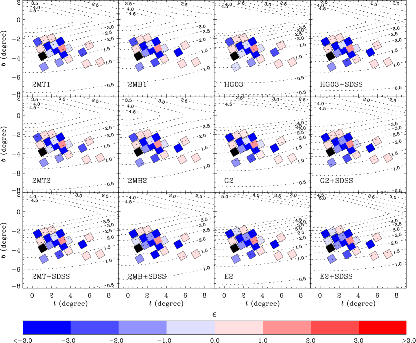
Figure 1: Relative difference of microlensing optical depths in $10^{-6}$ between MACHO results and models, normalized by the observational error $\sigma_{\tau}$, as a function of $(l,b)$. Note that the fields of negative $\epsilon$ and positive $\epsilon$ are shown in blue and red, respectively. For those of $\tau_{o}=0.0$, fields are marked by black. Dotted curves in each panel represent the microlensing optical depth contour of a model in units of $10^{-6}$. Each panel results from different mass models indicated in the lower left corner of the panel. See the text for the definition of the error-normalized difference and for model descriptions.

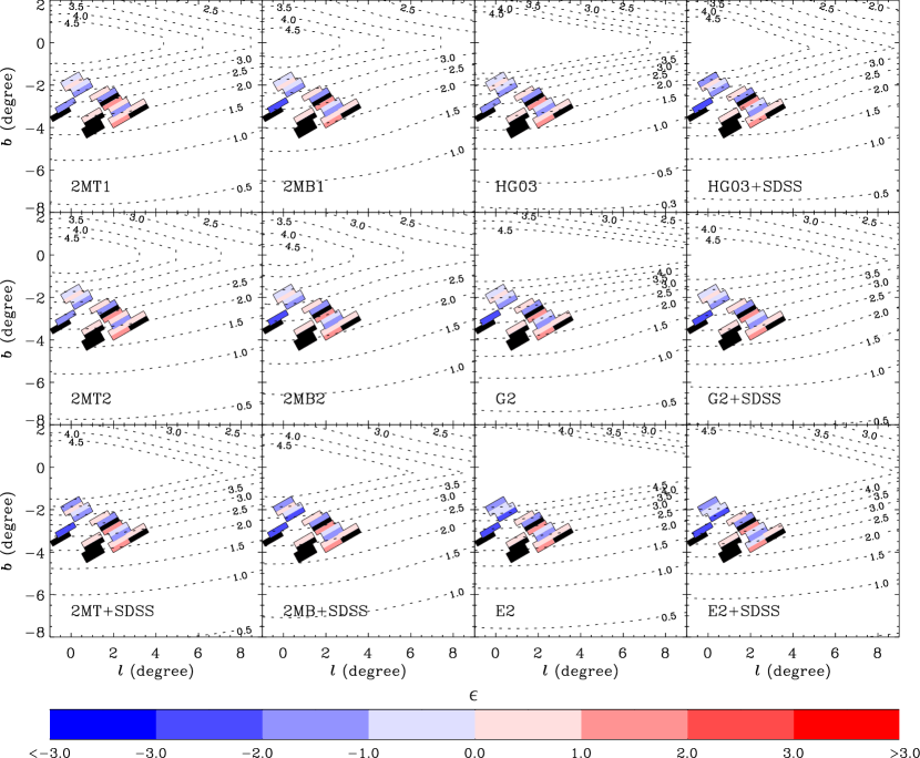
Figure 2: Same plots as Figure 1, but showing results from OGLE-II.

In Figures 1 and 2, we show the map of the optical depth difference normalized by the observational error $\sigma_{\tau}$ for each $(l,b)$ field, which is given by $\epsilon\equiv(\tau_{o}-\tau_{m})/\sigma_{\tau}$, where $\tau_{o}$ and $\tau_{m}$ are the microlensing optical depths in a given field from observation and model, respectively. We compare the microlensing optical depth observed from MACHO and OGLE-II with those calculated from models in field by field. Figures 1 and 2 result from MACHO and OGLE-II, respectively. In the map, the fields of negative $\epsilon$ and positive $\epsilon$ are shown in blue and red, respectively. For those of $\tau_{o}=0.0$, fields are marked by black. Dotted curves in each panel represent the microlensing optical depth contour of a model in units of $10^{-6}$. Each panel of Figures 1 and 2 results from different mass models indicated in the lower left corner of the panel. Table 1 summarize how to pair a bulge model and a disk model. For instance, 2MT1 and 2MB1 represent combinations of 2MASS triaxial bulge model and the 2MASS disk 1 model, 2MASS boxy bulge model and the 2MASS disk 1 model, respectively. In case of 2MT2 and 2MB2, the 2MASS disk 1 model is replaced by the 2MASS disk 2 model for a given bulge model. When the SDSS disk model is substituted, it is indicated as shown: HG03, G2, and E2 stand for cases of HG03, G2, and E2 bulge models and the disk model of Zheng et al. (2001).

To quantify the difference of the microlensing optical depth, we calculate $\chi^{2}_{l,b}$, defined as

$$\chi^{2}_{l,b}\equiv\sum^{N}_{i=1}\frac{(\tau_{o,i}-\tau_{m,i})^{2}}{\sigma_{o,i}^{2}},$$ (10)

where $\tau_{o,i}$, $\tau_{m,i}$ and $\sigma_{o,i}$ are the microlensing optical depths from observation and model, and the observational error in each field, respectively. Here summations are repeated over 14 OGLE-II fields and 19 MACHO fields excluding fields of $\tau_{o}=0$. We summarize results in Table 2. As seen, one finds that 2MASS, HG03, and G2 models agree well with the microlensing optical depth distribution for MACHO and OGLE-II when disk models of 2MASS and Zheng et al. (2001) are used. It should be noted that models that include the SDSS disk model produce relatively higher $\chi^{2}_{l,b}$ values. We note that the microlensing optical depth from MACHO has much higher $\chi^{2}_{l,b}$ values than OGLE-II since the microlensing optical depth values in four MACHO fields (176, 113,109, and 105) are 3$\sigma$ below with respect to the microlensing optical depth values expected from all models in those fields. Therefore, it should be pointed out that comparing two columns of OGLE-II and MACHO is meaningless. We repeat calculation of $\chi^{2}$ without those four fields and show results in parentheses for comparison in Table 2. Conclusion remains same. The reason why four of the MACHO fields deviate out of 3 $\sigma$ could be either that the models are too smooth to explain details of Galactic structures while there could be components affecting more optically than dynamically or that observational contaminations like the blending effect may play a role. For instance, OGLE-II investigates the blending effect even in bright events and points out that many bright microlensing events include heavily blended events (e.g. Udalski et al., 1994; Alcock et al., 1997b; Smith et al., 2007).

In Figure 3, we also show microlensing optical depths averaged over the Galactic longitude as a function of the Galactic latitude $b$. In the left panel, averages of microlensing optical depths measured by OGLE-II, MACHO, and EROS-2 are shown with their error bars. OGLE-II, MACHO, and EROS-2 data are plotted with filled circles, squares, and triangles, respectively. Best fits are superposed on top of observed data. Different line types represent different microlensing experiments: continuous, short dashed and long dashed lines stand for best-fit curves of OGLE-II, MACHO, and EROS-2, respectively. Analytic functions of those fits estimated by OGLE-II, MACHO, and EROS-2 are given as $\tau_{\rm{OGLE-II}}=[(4.48\pm 2.37)+(0.78\pm 0.84)\times b]\times 10^{-6}$ (Sumi et al., 2006), $\tau_{\rm{MACHO}}=[5.2+(1.06\pm 0.71)\times b]\times 10^{-6}$ (Popowski et al., 2005), and $\tau_{\rm{EROS-2}}=(1.62\pm 0.23)\exp[-(0.43\pm 0.16)(|b|-3\arcdeg)]\times 10^{-6}$ (Hamadache et al., 2006), respectively. In the right panel, microlensing optical depths toward the Galactic bulge expected from models described in the previous section are shown as a function of the Galactic latitude $b$ with thin curves. Dashed curve represents the calculated microlensing optical depth resulted from the 2MASS triaxial bulge model and the 2MASS disk 2 model (2MT2). Dotted curve represents the calculated microlensing optical depth resulted from the 2MASS boxy bulge model and the 2MASS disk 2 model (2MB2). Long dashed, dot-long-dashed, and dot-short-dashed curves represent HG03, G2, and E2 models, respectively. For comparison, we plot best fits obtained by different microlensing experiments with thick curves, which are already shown in the left panel. Continuous, short dashed and long dashed curves correspond to results of OGLE-II, MACHO, and EROS-2, respectively, as in the left panel. Models shown in the plot in general seem compatible with all the microlensing observations within the observational uncertainties. It is interesting to note that deviations among model fits become larger as the Galactic latitude decreases. To evaluate more quantitatively we calculate $\chi^{2}_{b}$ in each $b$ using equation (10), and list results in Table 3. As seen previously in Table 2, 2MASS, HG03, and G2 result in smaller $\chi^{2}_{b}$ in all the microlensing experiments. In Table 3 we show $\chi^{2}_{b}$ of all cases, including those not shown in the right panel of Figure 3. One may find again that when SDSS disk model is used fits become poorer.

4 SUMMARY AND DISCUSSIONS

By comparing the microlensing optical depth map constructed by a mass model with the observed microlensing optical depth one may put a tight constraint on the Galactic model. We have estimated the microlensing optical depths toward the Galactic bulge using the Galactic bulge and disk models constructed from survey observations, and compared them with the sample of microlensing events observed towards the Galactic bulge with red clump giant sources reported by the MACHO, OGLE-II and EROS-2 collaborations. From the analysis we carried out, we show that model estimates are in general compatible with microlensing observations. According to calculated $\chi^{2}$ we find that 2MASS, HG03, and G2 models reproduce the microlensing optical depth distribution from observations well. We also find that for those well-fit models contribution to the microlensing optical depth of the disk components is not crucial. For example, for 2MASS cases two disk models do not make any difference in $\chi^{2}$. It is, however, interesting to note that the analyses of SDSS disk models give us somewhat different results. That is, models including SDSS disk model produce relatively higher $\chi^{2}$ values than others do.

It should be pointed out that current observational data of both the microlensing optical depth in two dimensional fields and the averaged optical depth over $l$ are yet statistically insufficient to rule out conclusively any specific models we have considered since the number of observed microlensing events from monitoring RCGs in recent microlensing surveys is still small. On the other hands, we note that the difference of the average optical depth among models increases as closer to the Galactic center. Therefore, we suggest the microlensing observation toward closer to the Galactic center regions if possible may be more effective in constraining the Galactic model than extending microlensing searches to detect more microlensing events.

Table 1: Bulge and disk models

	2MASS disk 1	2MASS disk 2	Zheng disk	SDSS disk
2MASS triaxial bulge	2MT1	2MT2		2MT+SDSS
2MASS boxy bulge	2MB1	2MB2		2MB+SDSS
Han & Gould (2003)			HG03	HG03+SDSS
G2 of Stanek et al. (1997)			G2	G2+SDSS
E2 of Stanek et al. (1997)			E2	E2+SDSS

Table 2: The chi-square values of microlensing optical depths between observations and model estimates in two dimensional microlensing optical depth map.

	$\chi^{2}_{l,b}$
Model	OGLE-II	MACHO
2MT1	13.73	122.23 (27.20)
2MT2	13.57	122.31 (27.51)
2MT+SDSS	19.23	178.20 (38.76)
2MB1	15.24	143.84 (34.55)
2MB2	14.91	142.55 (34.63)
2MB+SDSS	21.84	208.89 (49.50)
HG03	14.90	121.72 (24.92)
HG03+SDSS	17.68	156.83 (32.77)
G2	16.81	159.30 (35.15)
G2+SDSS	20.13	202.00 (46.15)
E2	23.66	200.51 (41.89)
E2+SDSS	28.05	248.51 (54.15)

Note. — The number of fields used in the summation is 14 and 19 for OGLE-II and MACHO, respectively. For MACHO, chi-square values excluding 4 fields whose errors are greater than 3 $\sigma$ are also shown in parentheses for comparison.

Table 3: The chi-square values of averaged optical depths as a funciton of $b$.

	$\chi^{2}_{b}$
Model	OGLE-II	MACHO	EROS-2
2MT1	2.27	1.66	10.71
2MT2	2.26	1.76	10.57
2MT+SDSS	3.48	6.94	22.03
2MB1	2.76	4.41	18.41
2MB2	2.73	4.35	18.00
2MB+SDSS	4.81	13.41	35.59
HG03	2.41	1.76	10.83
HG03+SDSS	3.13	5.20	17.46
G2	3.30	6.25	21.11
G2+SDSS	4.54	12.05	31.55
E2	4.94	13.42	28.00
E2+SDSS	6.60	21.26	39.22

Figure 3: Averaged microlensing optical depths overthe Galactic longitude $l$ as a function of the Galactic latitude $b$. Left: Averages of microlensing optical depths measured by OGLE-II, MACHO, and EROS-2 are shown with their error bars. OGLE-II, MACHO, and EROS-2 data are plotted with filled circles, squares, and triangles, respectively. Continuous, short dashed, and long dashed lines stand for the best-fit curves of OGLE-II, MACHO, and EROS-2, respectively. Right: Microlensing optical depths toward the Galactic bulge expected from models are shown as a function of the Galactic latitude $b$ with thin curves. Dashed and dotted curves represent the calculated microlensing optical depth resulted from 2MT2 and 2MB2, respectively. Long-dashed, dot and long-dashed, and dot and short-dashed curves represent HG03, G2, and E2, respectively. For comparison, OGLE-II, MACHO, and EROS-2 microlensing experiment results are shown with thick continuous, short-dashed, and long-dashed curves.

References

- Afonso et al. (2003) Afonso, C., et al. 2003, A&A, 404, 145
- Alcock et al. (1993) Alcock C. et al. 1993, Nature, 365, 621
- Alcock et al. (1997a) Alcock, C., et al. 1997a, ApJ, 479, 119
- Alcock et al. (1997b) Alcock, C., et al. 1997b, ApJ, 486, 697
- Ansari et al. (1999) Ansari, R., et al. 1999, A&A, 344, L49
- Aubourg et al. (1993) Aubourg, E., et al. 1993, Nature, 365, 623
- Binney et al. (2000) Binney, J., Bissantz, N., & Gerhard, O. 2000, ApJ, 537, L99
- Blum (1995) Blum, R. D. 1995, ApJ, 444, L89
- Calchi Novati et al. (2005) Calchi Novati, S., et al. 2005, A&A, 443, 911
- Calchi Novati et al. (2008) Calchi Novati, S., et al. 2008, A&A, 480, 723
- de Jong et al. (2004) de Jong, J. T. A., et al. 2004, A&A, 417, 461
- Dehnen & Binney (1998) Dehnen, W., & Binney, J. 1998, MNRAS, 294, 429
- Dwek et al. (1995) Dwek, E., et al. 1995, ApJ, 445, 716
- Hamadache et al. (2006) Hamadache, C., et al. 2006, A&A, 454, 185
- Han Gould (1995) Han, C., Gould, A. 1995, ApJ, 449, 521
- Han Gould (2003) Han, C., Gould, A. 2003, ApJ, 592, 172
- Holtzman et al. (1998) Holtzman, J. A., Watson, A. M., Baum, W. A., Grillmair, C. J., Groth, E. J., Light, R. M., Lynds, R., & O’Neil, E. J., Jr. 1998, AJ, 115, 1946
- Jurić et al. (2008) Jurić, M., et al. 2008, ApJ, 673, 864
- Kerins et al. (2006) Kerins, E., Darnley, M. J., Duke, J. P., Gould, A., Han, C., Jeon, Y.-B., Newsam, A., & Park, B.-G. 2006, MNRAS, 365, 1099
- Kiraga Paczyński (1994) Kiraga, M., Paczyński, B. 1994, ApJ, 430, L101
- López-Corredoira et al. (2004) López-Corredoira, M., Cabrera-Lavers, A., Gerhard, O. E., & Garzón, F. 2004, A&A, 421, 953
- López-Corredoira et al. (2005) López-Corredoira, M., Cabrera-Lavers, A., & Gerhard, O. E. 2005, A&A, 439, 107
- Paczyński (1986) Paczyński, B. 1986, ApJ, 304, 1
- Paczyński et al. (1994) Paczyński, B., Stanek, K. Z., Udalski, A., Szymanski, M., Kaluzny, J., Kubiak, M., Mateo, M., & Krzeminski, W. 1994, ApJ, 435, L113
- Popowski et al. (2001) Popowski, P., et al. 2001, Microlensing 2000: A New Era of Microlensing Astrophysics, 239, 244
- Popowski et al. (2005) Popowski, P., et al. 2005 ApJ, 631, 879
- Riffeser et al. (2003) Riffeser, A., Fliri, J., Bender, R., Seitz, S., & Gössl, C. A. 2003, ApJ, 599, L17
- Skrutskie et al. (1997) Skrutskie, M. F., et al. 1997, The Impact of Large Scale Near-IR Sky Surveys, 210, 25
- Stanek et al. (1997) Stanek K., Z., et al. 1997, ApJ, 477, 163
- Smith et al. (2007) Smith, M. C., Woźniak, P., Mao, S., & Sumi, T. 2007, MNRAS, 380, 805
- Sumi et al. (2006) Sumi, T., et al. 2006, ApJ, 636, 240
- Udalski et al. (1994) Udalski, A., et al. 1994, Acta Astronomica, 44, 165
- Uglesich et al. (2004) Uglesich, R. R., Crotts, A. P. S., Baltz, E. A., de Jong, J., Boyle, R. P., & Corbally, C. J. 2004, ApJ, 612, 877
- Weiland et al. (1994) Weiland, J. L., et al. 1994, ApJ, 425, L81
- Wood & Mao (2005) Wood, A., & Mao, S. 2005, MNRAS, 362, 945
- Wood (2007) Wood, A. 2007, MNRAS, 380, 901
- York et al. (2000) York, D. G., et al. 2000, AJ, 120, 1579
- Zhao et al. (1995) Zhao, H., Spergel, D. N., & Rich, R. M. 1995, ApJ, 440, L13
- Zhao & Mao (1996) Zhao, H., & Mao, S. 1996, MNRAS, 283, 1197
- Zhao et al. (1996) Zhao, H., Rich, R. M., & Spergel, D. N. 1996, MNRAS, 282, 175
- Zheng et al. (2001) Zheng, Z., Flynn, C., Gould, A., Bahcall, J. N., & Salim, S. 2001, ApJ, 555, 393
- Zoccali et al. (2000) Zoccali, M., Cassisi, S., Frogel, J. A., Gould, A., Ortolani, S., Renzini, A., Rich, R. M., & Stephens, A. W. 2000, ApJ, 530, 418