$ZZ\rightarrow\ell^{+}\ell^{-}\nu\bar{\nu}$ production in $p\bar{p}$ collisions at $\sqrt{s}$= 1.96 TeV

Abstract

We describe a search for $Z$ boson pair production in $p\bar{p}$ collisions at $\sqrt{s}$= 1.96 TeV with the D0 detector at the Fermilab Tevatron Collider using a data sample corresponding to an integrated luminosity of 2.7 fb^-1. Using the final state decay $ZZ\rightarrow\ell^{+}\ell^{-}\nu\bar{\nu}$ (where $\ell=e$ or $\mu$) we find a signal with a 2.6 standard deviations significance (2.0 expected) corresponding to a cross section of $\sigma(p\bar{p}\rightarrow ZZ+X)=2.01\pm 0.93\mathrm{(stat.)}\pm 0.29\mathrm{(sys.)}$ pb.

I Introduction

We report a search for $Z$ boson pair production in $p\bar{p}$ collisions in the mode where one $Z$ boson decays into two charged leptons (either electrons or muons) and the other $Z$ boson decays into two neutrinos (see Fig. 1). In the Standard Model (SM), $ZZ$ production is the double gauge boson process with the lowest cross section and is the last remaining unobserved diboson process at the Tevatron, aside from the expected associated production of the Higgs boson. Observation of $ZZ$ production therefore represents an essential step in Higgs boson searches in the $ZH$ and $WH$ channels with sensitivity at the level of the expected SM cross sections. Additionally, the $ZZ$ process forms a background to Higgs boson searches, for example in the channels $ZH\rightarrow\ell^{+}\ell^{-}b\overline{b}$, $ZH\rightarrow\nu\overline{\nu}b\overline{b}$ and $H\rightarrow W^{+}W^{-}\rightarrow\ell^{+}\nu\ell^{-}\overline{\nu}$. Unlike the $WW$ and $WZ$ processes, there are no expected SM contributions from triple gauge boson couplings involving two $Z$ bosons and a measurement of the $ZZ$ cross section represents a test for production of this final state via anomalous couplings.

The process $ZZ\rightarrow\ell^{+}\ell^{-}\nu\bar{\nu}$ has a branching ratio six times larger than that for the other purely leptonic process $ZZ\rightarrow\ell^{+}\ell^{-}\ell^{\prime+}\ell^{\prime-}$. After removing instrumental backgrounds, the dominant background in the $ZZ\rightarrow\ell^{+}\ell^{-}\nu\bar{\nu}$ search arises from the process $WW\rightarrow\ell^{+}\nu\ell^{-}\bar{\nu}$, which produces the same final state particles. A kinematic discriminant against background from $WW\rightarrow\ell^{+}\nu\ell^{-}\bar{\nu}$ is employed. In contrast, a search in the $ZZ\rightarrow\ell^{+}\ell^{-}\ell^{\prime+}\ell^{\prime-}$ channel benefits from having no significant backgrounds from physics processes with the same final state.

We select events containing an electron or muon pair with high invariant mass and significant missing transverse momentum. After the initial event selection, the dominant source of instrumental background to this signature arises from events containing a leptonic $Z$ boson decay in which the apparent missing transverse momentum arises from mismeasurement of the transverse momentum of either the charged leptons or the hadronic recoil system. We introduce a variable that is highly discriminating against such instrumental background.

Although the $e^{+}e^{-}\rightarrow ZZ$ process has been observed at LEP LEPZZ , $ZZ$ production has not yet been observed at a hadron collider where different physics processes are allowed and higher energies can be probed. The D0 collaboration has previously performed a search for the process $ZZ\rightarrow\ell^{+}\ell^{-}\ell^{\prime+}\ell^{\prime-}$ with $\ell,\ell^{\prime}=e\ \mathrm{or}\ \mu$ b-d0 , which set a limit on the cross section of $\sigma(ZZ)<4.4$ pb and also examined non SM triple gauge boson couplings. The CDF collaboration has recently produced a result using both the $\ell^{+}\ell^{-}\ell^{\prime+}\ell^{\prime-}$ and the $\ell^{+}\ell^{-}\nu\bar{\nu}$ channels b-cdf , measuring the cross section to be $\sigma(ZZ)=1.4^{+0.7}_{-0.6}$ pb.

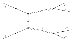
Figure 1: Leading order Feynman diagram for the process $ZZ\rightarrow\ell^{+}\ell^{-}\nu\bar{\nu}$.

The D0 detector nim1 ; nim2 ; nimmu contains tracking, calorimeter and muon subdetector systems. Silicon microstrip tracking detectors (SMT) near the interaction point cover pseudorapidity $|\eta|<3$ to provide tracking and vertexing information. The SMT contains cylindrical barrel layers aligned with their axes parallel to the beams and disk segments. The disks are perpendicular to the beam axis, interleaved with, and extending beyond, the barrels. The central fiber tracker (CFT) surrounds the SMT, providing coverage to about ($|\eta|=2$). The CFT has eight concentric cylindrical layers of overlapped scintillating fibers providing axial and stereo ($\pm 3^{\circ}$) measurements. A 2 T solenoid surrounds these tracking detectors. Three uranium-liquid argon calorimeters measure particle energies. The central calorimeter (CC) covers $|\eta|<1$, and two end calorimeters (EC) extend coverage to about $|\eta|=4$. The calorimeter is highly segmented along the particle direction, with four electromagnetic (EM) and four to five hadronic sections, and transverse to the particle direction with typically $\Delta\eta=\Delta\phi=0.1$, where $\phi$ is the azimuthal angle. The calorimeters are supplemented with central and forward scintillating strip preshower detectors (CPS and FPS) located in front of the CC and EC. Intercryostat detectors (ICD) provide added sampling in the region $1.1<|\eta|<1.4$ where the CC and EC cryostat walls degrade the calorimeter energy resolution. Muons are measured with stations which use scintillation counters and several layers of tracking chambers over the range $|\eta|<2$. One such station is located just outside the calorimeters, with two more outside $1.8$ T iron toroidal magnets. Scintillators surrounding the exiting beams allow determination of the luminosity. A three level trigger system selects events for data logging at about 100 Hz. The first level trigger (L1) is based on fast custom logic for several subdetectors and is capable of making decisions for each beam crossing. The second level trigger (L2) makes microprocessor based decisions using multi-detector information. The third level trigger (L3) uses fully digitized outputs from all detectors to refine the decision and select events for offline processing.

II Data Set and Initial Event Selection

The data for this analysis were collected with the D0 detector at the Fermilab Tevatron $p\bar{p}$ Collider at a center-of-mass energy $\sqrt{s}=1.96$ TeV. An integrated luminosity of 2.7 fb^-1 is used after applying data quality requirements. The data are selected using a combination of single electron or single muon triggers for the respective dilepton channels.

The data taking period prior to March 2006 is refered to as Run IIa, while IIb denotes the period after. This division corresponds to the installation of an additional silicon vertex detector, trigger upgrades, and a significant increase in the rate of delivered luminosity.

In each of the two channels we require that there be exactly two oppositely charged leptons with transverse momentum $p_{T}>15$ GeV and dilepton invariant mass $70<M_{\ell\ell}<110$ GeV. Electrons are required to be within the central ($|\eta|<1.1$) or forward ($1.5<|\eta|<2.5$) regions of the calorimeter. We do not use electron candidates which point towards the transition region of the central and forward cryostats. Electrons must pass tight selection criteria on the energy close to them in $\Delta R$, where $\Delta R$ is the distance between two objects in $(\eta,\phi)$ space, $\Delta R=\sqrt{(\delta\phi)^{2}+(\delta\eta)^{2}}$, by requiring that

$$\frac{E_{\mathrm{tot}}(0.4)-E_{\mathrm{EM}}(0.2)}{E_{\mathrm{EM}}(0.2)}<0.15,$$

where $E_{\mathrm{tot}}(0.4)$ is the total energy within a cone of $\Delta R<0.4$ and $E_{EM}(0.2)$ is the EM energy within a cone of $\Delta R<0.2$. Additionally, a seven parameter multivariate discriminator compares the energy deposited in each layer of the calorimeter and the total shower energy to distributions determined from electron geant Monte Carlo (MC) simulations b-geant . This discriminator also uses the correlations between the various energy distributions to ensure that the shower shape is consistent with that produced by an electron.

Each muon is required to have an associated track in the central tracking system which has at least one hit in the SMT and a distance of closest approach to the primary vertex in the plane transverse to the beam of $|b|<0.02$ cm. Furthermore, the muons must be isolated in both the calorimeter and the tracker. For the former, a requirement is made that the sum of calorimeter energies in cells within an annulus $0.1<\Delta R<0.4$ around the muon track is smaller than 10% of the muon $p_{T}$:

$$\Sigma^{cells}E_{T}(0.1<\Delta R<0.4)/p_{T}(\mu)<0.1.$$

For the latter, the sum of track $p_{T}$ within a cone $\Delta R<0.5$ around the muon track (not included in the sum) must be smaller than 10% of the muon $p_{T}$:

$$\Sigma^{track}p_{T}(\Delta R<0.5)/p_{T}(\mu)<0.1.$$

To suppress background from $WZ$ production, we veto events with one or more leptons (e, $\mu$, or $\tau$) in addition to those forming the $Z$ candidate. Additional lepton candidates must be separated by $\Delta R>0.2$ from both $Z$–candidate leptons. Electron candidates used in the veto must have $E_{T}>5$ GeV and either a central track match or satisfy shower shape requirements. Muons are rejected based on looser quality requirements than those from $Z$ decay. Multi-prong hadronic taus are used to form the veto if they have been identified using the standard D0 algorithms b-d0tau . Finally, events are vetoed if they have any isolated tracks with $p_{T}>5$ GeV and a separation distance between the track intercept with the beam line and the primary vertex satisfying $|\Delta z|<1$ cm.

Events with relatively large calorimeter activity are rejected by vetoing on the presence of more than two jets in the detector. These jets are reconstructed using the Runn IIa cone algorithm jetcone with a radius of 0.5 and must satisfy $\Delta R$(jet, lepton)$>0.3$ and jet $E_{T}>15$ GeV. This requirement significantly reduces background from $t\overline{t}$ production.

Missing transverse energy ($\not\!\!E_{T}$) is the magnitude of the vector sum of transverse energy above a set threshold in the calorimeter cells, corrected for the jets in the event. At the dilepton selection stage, we do not make a requirement on $\not\!\!E_{T}$.

III Background and Signal Prediction

Background yields were estimated using a combination of control data samples and MC simulation. The primary background after the initial selection is inclusive $Z/\gamma^{*}\rightarrow\ell^{+}\ell^{-}$ production. After making the final selection described later, the dominant background is $W^{+}W^{-}\rightarrow\ell^{+}\nu\ell^{-}\overline{\nu}$ events. Additional backgrounds include $t\overline{t}$ production, $WZ$ production and $W\gamma$ or $W$+jets events in which the $\gamma$ or jet is misidentified as an electron.

The $WW$, $WZ$, $Z/\gamma^{*}$, and $t\bar{t}$ backgrounds are estimated based on simulations using the pythia b-pythia event generator, with the leading order CTEQ6L1 b-cteq parameterization used for the parton distribution functions (PDFs). We pass the simulated events through a detailed D0 detector simulation based on geant and reconstruct them using the same software program used to reconstruct the collider data. The $Z/\gamma^{*}$ MC events are assigned a weight as a function of generator level $p_{T}$, to match the $p_{T}$ spectrum observed in unfolded data zpt . Randomly triggered collider data events are added to the simulated pythia events. These data events are taken at various instantaneous luminosities to provide a more accurate modeling of effects related to the presence of additional $p\bar{p}$ interactions and detector noise. We also apply corrections for trigger efficiency, reconstruction efficiency and identification efficiency. The corrections are derived from comparisons of control data samples with simulation.

The $W\gamma$ background is estimated from a calculation of the Next to Leading Order (NLO) production cross section b-baur , which we use to normalize events generated by pythia. The probability for a photon to be misidentified as an electron is measured in a $Z\rightarrow\ell^{+}\ell^{-}\gamma$ control data sample. This probability is then applied to the $W\gamma$ yield predicted from simulation to determine the contribution to our selected sample in which the photon is mistakenly reconstructed as the second electron.

The kinematic distributions of the $W$+jet events are determined from simulation based on alpgen b-alpgen . The overall yield from $W$+jet events is determined from data. The probabilities that an electron or a jet which satisfy looser selection requirements will also pass our candidate selection in data are measured by solving a set of linear equations involving these probabilities, the number of candidate events, and the number of events in which one of the requirements on one of the candidates has been loosened. The solution to this set of linear equations is used to determine the number of $W$+jet events in the final sample. The fraction of jets misidentified as electrons is  $2\times 10^{-3}$, and the probability that a jet fakes a muon is  $4\times 10^{-4}$ (averaging over Run IIa and Run IIb).

The relative normalization of the background sources determined from simulation is taken from ratios of NLO cross sections, and the absolute normalization of the total background is then determined by matching the observed yield under the $Z$ dilepton mass peak to the predicted background sum after applying the basic $Z$ selection and extra–activity event veto. We choose this normalization method because inclusive $Z$ production dominates our signal by four orders of magnitude, and this approach allows cancellation of multiplicative scale uncertainties and systematics related to the modeling of the selection efficiencies. The normalization factor agrees with that obtained using the integrated luminosity to within the associated 6% uncertainty.

Signal events were generated using pythia with the CTEQ6L1 PDFs, and the signal event samples were corrected for the same detector effects as the background samples.

IV Verification of Missing Transverse Momentum

The basic event signature for this analysis is a high mass pair of charged leptons from the decay of a $Z$ boson, produced in association with significant missing transverse momentum $\not\!\!E_{T}$ arising from the neutrinos produced in the decay of a second $Z$ boson. Substantial background comes from single inclusive $Z$ production in which mismeasurement results in a mistakenly large $\not\!\!E_{T}$ value. Because the cross section times branching ratios for inclusive $Z$ production and $ZZ$ signal differ by a factor of more than $10^{4}$, stringent selection criteria against inclusive $Z$ production are required. We present a novel approach to this challenge. In particular, we do not attempt to make an unbiased or accurate estimate of the missing transverse momentum in the candidate events. Rather, our approach is to construct a variable $\not\!\!E^{\prime}_{T}$ which is a representation of the minimum $\not\!\!E_{T}$ feasible given the measurement uncertainties of the leptons and the hadronic recoil. Thus, this is not intended to be the best estimator of true $\not\!\!E_{T}$, but rather to be robust against reconstruction mistakes. This approach is inspired by the OPAL collaboration which used a similar variable to search in final states similar to that of this analysis OPAL .

The $\not\!\!E^{\prime}_{T}$ variable is constructed in five steps.

1. The first step is the computation of a reference axis chosen such that effects from leptonic resolution occur dominantly along this axis, and the decomposition of the dilepton system transverse momentum into components parallel and perpendicular to this reference axis.

2. The second step is determination of a recoil variable based on measured calorimeter jet or total calorimeter activity. In events with no significant neutrino energy or mismeasurement, the quantities calculated in the first two steps should be approximately balanced.

3. The third step is the calculation of a correction based on recoil track $p_{T}$ for tracks which are well separated from the candidate leptons and calorimeter jets.

4. The fourth step is the computation of a correction term accounting for lepton transverse momentum measurement uncertainties.

5. The final step is a combination of the quantities computed in the first four steps into the $\not\!\!E^{\prime}_{T}$ variable.

IV.1 Decomposition

In the first step, to minimize the sensitivity to mismeasurement of the $p_{T}$ of the individual leptons, the $\vec{p}_{T}$ of the lepton pair is decomposed into two components, one of which is almost insensitive to lepton $p_{T}$ resolution for $Z$ candidates with moderate values of transverse momentum. This decomposition is achieved as follows. In the transverse plane a dilepton thrust axis is defined (see Fig. 2).

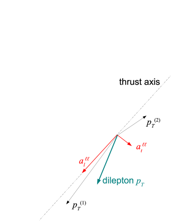
Figure 2: Representation of the transverse plane of the event and of the decomposition of the dilepton transverse momentum along the thrust axis.

This axis maximizes the scalar sum of the projections of the $p_{T}$ of the two leptons onto the axis. It is defined as

$$\vec{t}=\vec{p}_{T}^{\ (1)}-\vec{p}_{T}^{\ (2)},$$

where $\vec{p}_{T}^{\ (1)}$ and $\vec{p}_{T}^{\ (2)}$ are the transverse momenta of the higher and lower $p_{T}$ leptons respectively.

We then define two unit vectors $\hat{a_{l}}$ and $\hat{a_{t}}$ which are parallel and perpendicular to the thrust axis. For the rest of this paper, a subscript $l$ denotes the component in the $\hat{a_{l}}$ directio and a subscript $t$ denotes the component of a vector in the $\hat{a_{t}}$ direction.

The dilepton system transverse momentum is decomposed into components parallel to $\hat{a_{l}}$ ($a_{l}^{\ell\ell}$) and perpendicular to $\hat{a_{l}}$ ($a_{t}^{\ell\ell}$). These are given by

$$a_{t}^{\ell\ell} = \vec{p}_{T}^{\ \ell\ell}\cdot\hat{a_{t}}$$

$$a_{l}^{\ell\ell} = \vec{p}_{T}^{\ \ell\ell}\cdot\hat{a_{l}},$$

in which $\vec{p}_{T}^{\ \ell\ell}\equiv\vec{p}_{T}^{\ (1)}+\vec{p}_{T}^{\ (2)}$ is the dilepton system transverse momentum. The resolutions of the two components are shown in Fig. 3 from $Z\rightarrow\mu\mu$ (MC) generated events. Resolution effects are more pronounced in the $Z\rightarrow\mu\mu$ channel than in the $Z\rightarrow ee$. As seen, the lepton momentum resolution effects are significantly more pronounced in the $\hat{a_{l}}$ direction than in the $\hat{a_{t}}$ direction.

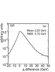
Figure 3: The difference between measured and true dilepton $p_{T}$ in simulated $Z\rightarrow\mu\mu$ events projected along the (a) $\hat{a_{l}}$ and (b) $\hat{a_{t}}$ axes.

The decomposition is performed only for events in which $\Delta\phi^{\ell\ell}>\pi/2$, where $\Delta\phi^{\ell\ell}$ is the angle between the two charged leptons in the transverse plane. For the case $\Delta\phi^{\ell\ell}\leq\pi/2$ the direction of the dilepton transverse momentum $\vec{p}_{T}^{\ \ell\ell}$ is used to define $\hat{a_{t}}$, and all components in the $\hat{a_{l}}$ direction are set to zero.

IV.2 Calorimeter Recoil Activity

The second step in the process uses calorimeter energy to assess whether or not it might generate apparent, though false, $\not\!\!E_{T}$. Two measures of net calorimeter transverse energy are considered: (a) a vector sum of the $E_{T}$ of selected reconstructed jets and (b) the uncorrected missing transverse energy $\not\!\!E_{T}$ for the event from the calorimeter. When computing the jet $\vec{p}_{T}$ sum, we consider only those jets whose $p_{T}$ is in the direction opposite to the dilepton system for each of the $\hat{a_{l}}$ and $\hat{a_{t}}$ directions. That is, if $\vec{p}_{T}^{\ jet}\cdot\hat{a_{l}}<0$, then this amount is added to the $\hat{a_{l}}$ correction, and if $\vec{p}_{T}^{\ jet}\cdot\hat{a_{t}}<0$, it is added to the $\hat{a_{t}}$ correction.

The calorimeter activity correction is then defined using either the jets or the uncorrected $\not\!\!E_{T}$. We chose the one with the largest projected magnitude along each of the two axes in the hemisphere opposite to the dilepton pair. Additionally, we allow for the possibility that only some of the true recoiling energy is underestimated by multiplying the observed energy by two. The calorimeter correction is thus defined as

$$\delta a_{t}^{cal} = 2\times\mathrm{min}(\Sigma\vec{p_{T}}^{jets}\cdot\hat{a_{t}},-\vec{\mbox{$\not\!\!E_{T}$}}\cdot\hat{a_{t}},0)$$

$$\delta a_{l}^{cal} = 2\times\mathrm{min}(\Sigma\vec{p_{T}}^{jets}\cdot\hat{a_{l}},-\vec{\mbox{$\not\!\!E_{T}$}}\cdot\hat{a_{l}},0)$$

in which a jet is used in the $\hat{a_{l}}(\hat{a_{t}})$ component sum only if it satisfies $\vec{p}_{T}\cdot\hat{a_{l}}<0\ (\vec{p}_{T}\cdot\hat{a_{t}}<0)$. The presence of the zero term in the $\mathrm{min}$–function ensures that the calorimeter activity correction is used only if it decreases the apparent value of $a_{t}^{\ell\ell}$ and/or $a_{l}^{\ell\ell}$. In this way we try to minimize the possibility that a well-balanced event acquires an apparently significant net missing momentum due to calorimeter noise or a jet with a grossly overestimated energy.

IV.3 Recoiling Tracks

The third step identifies events in which the recoil activity is not observed in the calorimeter as jets. We consider tracks that are $\Delta R>0.5$ away from all calorimeter jets, $\Delta R>0.5$ from the candidate leptons, have a fit satisfying ${\chi^{2}}/{\mathrm{NDF}}<4.0$, and $p_{T}>0.5$ GeV and use these to build track jets using a cone algorithm. A track jet is seeded by the highest $p_{T}$ track not yet associated with any track jet. All tracks which are within $\Delta R<0.5$ of the seed track and are not yet associated with a track jet are added to the current track jet. The track jet transverse momentum $p_{T}^{tjet}$ is the vector sum of the $p_{T}$ values of all tracks forming the track jet. This is repeated until no unused tracks outside the calorimeter jet cones remain. A track–based correction is then defined as

$$\delta a_{t}^{trk} = (\Sigma\vec{p}_{T}^{\ tjet})\cdot\hat{a_{t}}$$

$$\delta a_{l}^{trk} = (\Sigma\vec{p}_{T}^{\ tjet})\cdot\hat{a_{l}}.$$

As with the calorimeter jets, a track jet is included in the correction for the $\hat{a_{l}}(\hat{a_{t}})$ direction only if it satisfies $\vec{p}_{T}^{\ tjet}\cdot\hat{a_{l}}<0\ (\vec{p}_{T}^{\ tjet}\cdot\hat{a_{t}}<0)$.

IV.4 Lepton $p_{T}$ Uncertainty

In the fourth step of the algorithm, corrections $\delta a_{t}^{\ell\ell}$ and $\delta a_{l}^{\ell\ell}$ arising from the uncertainties in the lepton transverse momenta are derived. The basic approach taken is to fluctuate the lepton transverse momenta by one standard deviation of their uncertainty so as to minimize, separately, the $\hat{a_{l}}$ and $\hat{a_{t}}$ components of the dilepton $p_{T}^{\ell\ell}$. The transverse component, $a_{t}^{\ell\ell}$, is minimized by decreasing the transverse momenta of both leptons to give the modified quantity:

$$a_{t}^{\ell\ell^{\prime}}=\vec{p}_{T}^{\ \ell\ell^{\prime}}\cdot\hat{a_{t}}^{\prime}.$$

Here $\vec{p}_{T}^{\ \ell\ell^{\prime}}$ and $\hat{a_{t}}^{\prime}$ correspond, respectively, to $\vec{p}_{T}^{\ \ell\ell}$ and $\hat{a_{t}}$, redefined using $\vec{p}_{T}^{\ (1)}\times(1-\sigma_{1})$ and $\vec{p}_{T}^{\ (2)}\times(1-\sigma_{2})$ in place of the unscaled quantities. The uncertainty is then simply given by:

$$\delta a_{t}^{\ell\ell}=a_{t}^{\ell\ell^{\prime}}-a_{t}^{\ell\ell}.$$

The longitudinal component, $a_{l}^{\ell\ell}$, is minimized by decreasing $\vec{p}_{T}^{\ (1)}$ and increasing $\vec{p}_{T}^{\ (2)}$ using their fractional uncertainties $\sigma_{1}$ and $\sigma_{2}$:

$$\delta a_{l}^{\ell\ell}=(-\sigma_{1}\vec{p}_{T}^{\ (1)}+\sigma_{2}\vec{p}_{T}^{\ (2)})\cdot\hat{a_{l}}$$

If the fractional uncertainty on either of the lepton transverse momenta is larger than unity, then the fractional uncertainties on both $a_{t}^{\ell\ell}$ and $a_{l}^{\ell\ell}$ are set to unity.

Electrons falling at calorimeter module boundaries of the central calorimeter require special treatment as their calculated uncertainties do not reflect the probability for such electrons to have very significantly underestimated energies. To account for this, if the lower $p_{T}$ electron is within a central calorimeter module boundary, then the fractional uncertainty on $a_{l}^{\ell\ell}$ is set to unity.

IV.5 Combination

In the fifth and final step, the variable $\not\!\!E^{\prime}_{T}$ is computed from the quantities calculated in the previous steps. We compute components:

$$a_{t} = a_{t}^{\ell\ell}+\delta a_{t}^{cal}+k^{\prime}\times\delta a_{t}^{trk}+k\times\delta a_{t}^{\ell\ell}$$

$$a_{l} = a_{l}^{\ell\ell}+\delta a_{l}^{cal}+k^{\prime}\times\delta a_{l}^{trk}+k\times\delta a_{l}^{\ell\ell},$$

where $k$ and $k^{\prime}$ are constants defined below. Recall that by construction the $\delta a_{i}$ (where $i=t$ or $l$) terms are always zero or negative while $a_{i}^{\ell\ell}$ is positive.

For events with significant transverse energy from neutrinos and no mismeasurements, the $a_{i}$ variables are large and positive. If $a_{i}\leq 0$, then there is no significant missing transverse momentum along direction $i$ and that component is ignored in the subsequent analysis by setting:

$$a_{t}^{\prime} = \mathrm{max}(a_{t},0),$$

$$a_{l}^{\prime} = \mathrm{max}(a_{l},0).$$

The final discriminating variable is then calculated as a weighted quadrature sum of the two components:

$${\mbox{$\not\!\!E^{\prime}_{T}$}}=\sqrt{a_{l}^{\prime 2}+(1.5a_{t}^{\prime})^{2}}.$$

By construction $\not\!\!E^{\prime}_{T}$ is less that $\not\!\!E_{T}$. The factor of $1.5$ is used with the $\hat{a_{t}}$ component to give extra weight to the better–measured direction. As mentioned earlier, if $\Delta\phi^{\ell\ell}<\pi/2$, then instead of using the thrust axis, the reference axis direction $\hat{a_{t}}$ is simply the $\vec{p}_{T}^{\ \ell\ell}$ direction, and the $\hat{a_{l}}$ components are ignored.

The values $k$ and $k^{\prime}$ were optimized by applying a loose cut in $\not\!\!E^{\prime}_{T}$ (such that the background in the sample is dominated by $Z\rightarrow\ell^{+}\ell^{-}$ events) and maximizing $S/\sqrt{B}$, where $S$ is the number of signal events and $B$ is the number of background events. The chosen values for dielectron events are $k=2.2$ and $k^{\prime}=2.5$. For dimuon events, $k=k^{\prime}=1.5$.

The power of the variable $\not\!\!E^{\prime}_{T}$ is displayed in Figure 4, which shows the distribution of $\not\!\!E^{\prime}_{T}$, for the dielectron and dimuon channels separately.

The separation of sources with true $\not\!\!E_{T}$ (e.g. $WW$ and $ZZ$) from those without, especially inclusive $Z$ production, is clearly visible. The rejection of events from single $Z$ boson production using this method and a simple $\not\!\!E_{T}$ cut is shown in Figure 5.

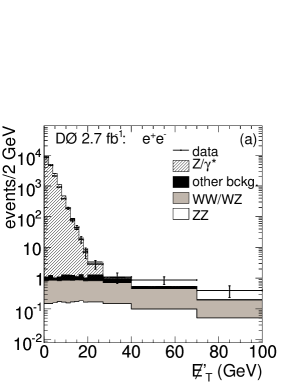
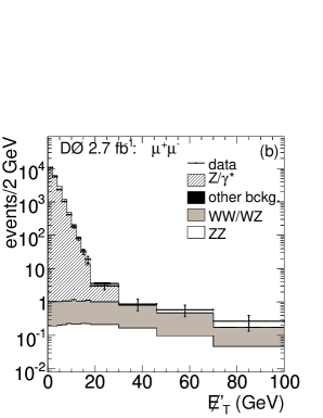
Figure 4: The $\not\!\!E^{\prime}_{T}$ distributions for dielectron (a) and dimuon (b) events.

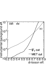
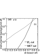
Figure 5: The efficiency of $WW$, $WZ$, and $ZZ$ events vs single $Z$ events using the $\not\!\!E_{T}$ (labeled as MET in the figure) and $\not\!\!E^{\prime}_{T}$ variables in the dielectron (a) and dimuon (b) channels.

V Final Selection, Likelihood and Yields

In addition to the initial selection requirements, events selected for further analysis must satisfy,

$$\not\!\!E^{\prime}_{T} > 27\ \mathrm{GeV,\ dielectron,\ IIa},$$

$$\not\!\!E^{\prime}_{T} > 30\ \mathrm{GeV,\ dimuon,\ IIa},$$

$$\not\!\!E^{\prime}_{T} > 27\ \mathrm{GeV,\ dielectron,\ IIb},$$

$$\not\!\!E^{\prime}_{T} > 35\ \mathrm{GeV,\ dimuon,\ IIb}.$$

The values of these requirements were chosen so as to optimize the expected significance of a $ZZ$ observation in the four individual analysis channels, assuming the SM cross sections for signal and backgrounds. The effect of systematic uncertainties, as described below, were used in the significance calculation for the optimization. Tables 1 and 2 show the predicted and observed yields after the initial selection and after the $\not\!\!E^{\prime}_{T}$ selection for the dielectron and dimuon channels respectively. The requirement on $\not\!\!E^{\prime}_{T}$ reduces the predicted instrumental background yields well below those for our signal and remaining physics backgrounds. In the dielectron channel, we observe 8 events (8.9 expected) in the IIa data, with another 20 events (10.7 expected) in the IIb data. Of these, we expect 1.8 and 2.3 to be signal events respectively. In the dimuon channel, we observe 10 events (7.0 expected) in the IIa data and 5 events (7.3 expected) in the IIb data. Here, we expect 1.7 signal events in each data set.

Table 1: Number of predicted dielectron events and yield observed in data after the dilepton selection and after the requirement on $\not\!\!E^{\prime}_{T}$. The uncertainties in the final column are statistical only. If not present, the statistical uncertainty is negligible.

Sample	dilepton selection	$\not\!\!E^{\prime}_{T}$ requirement
$Z\rightarrow\ell^{+}\ell^{-}$	$1.18\times 10^{5}$	0.5 $\pm$ 0.2
$Z\rightarrow\tau^{+}\tau^{-}$	48.3	0.35 $\pm$ 0.00
$W$+Jets	18.2	2.7 $\pm$ 0.4
$t\bar{t}$	16.4	0.34 $\pm$ 0.00
$WW$	28.0	10.6 $\pm$ 0.1
$WZ$	19.2	1.08 $\pm$ 0.00
$W\gamma$	2.0	0.03 $\pm$ 0.00
Predicted Background	$1.19\times 10^{5}$	15.6 $\pm$ 0.4
$ZZ\rightarrow\ell^{+}\ell^{-}\ell^{\prime+}\ell^{\prime-}$	2.9	0.02 $\pm$ 0.00
$ZZ\rightarrow\ell^{+}\ell^{-}\nu\bar{\nu}$	8.9	4.03 $\pm$ 0.00
Predicted Total	$1.19\times 10^{5}$	19.6 $\pm$ 0.4
Data	118,850	28

Table 2: Number of predicted dimuon events and yield observed in data after the dilepton selection and after the requirement on $\not\!\!E^{\prime}_{T}$. The uncertainties in the final column are statistical only. If not present, the statistical uncertainty is negligible.

Sample	dilepton selection	$\not\!\!E^{\prime}_{T}$ requirement
$Z\rightarrow\ell^{+}\ell^{-}$	$1.30\times 10^{5}$	0.1 $\pm$ 0.1
$Z\rightarrow\tau^{+}\tau^{-}$	53.3	0.09 $\pm$ 0.00
$W$+Jets	–	$<$ 0.01
$t\bar{t}$	16.0	0.21 $\pm$ 0.00
$WW$	32.0	9.7 $\pm$ 0.1
$WZ$	18.3	0.82 $\pm$ 0.00
Predicted Background	$1.30\times 10^{5}$	10.9 $\pm$ 0.3
$ZZ\rightarrow\ell^{+}\ell^{-}\ell^{\prime+}\ell^{\prime-}$	2.89	0.00 $\pm$ 0.00
$ZZ\rightarrow\ell^{+}\ell^{-}\nu\bar{\nu}$	9.48	3.39 $\pm$ 0.00
Predicted Total	$1.30\times 10^{5}$	14.3 $\pm$ 0.3
Data	127,960	15

The $ZZ$ signal is separated from the remaining backgrounds with significant $\not\!\!E^{\prime}_{T}$ using a likelihood with the following input variables: the invariant mass of the dilepton pair, $M_{\ell\ell}$ (for the dielectron channel), the $\chi^{2}$ probability resulting from a refit of the measured lepton momenta under the constraint that their dilepton mass gives the $Z$ mass (for the dimuon channel), the transverse momentum of the higher $p_{T}$ lepton, $\vec{p_{T}}^{(1)}$, the opening angle between the dilepton pair and the leading lepton, $\Delta\phi$, and the cosine of the negative lepton scattering angle in the dilepton rest frame, $\cos(\theta^{*})$. Figures 6 and 7 show the data and predicted distributions of the variables used in the likelihood for the dielectron and dimuon channels respectively. Fig. 8 shows the likelihood distributions for signal and backgrounds after all selection requirements.

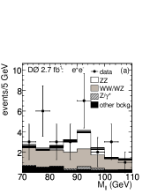
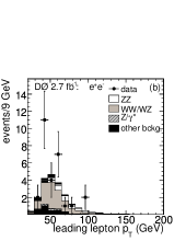
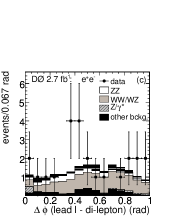
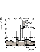
Figure 6: Distribution in the dielectron channel of the input variables of the likelihood discriminant for data and MC. Invariant mass of the dilepton system (a), $p_{T}$ of the leading lepton (b), the opening angle between the lead lepton and the dilepton system (c), and the cosine of the scattering angle of the negative lepton in the dilepton rest frame (d).

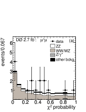
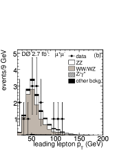
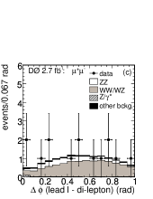
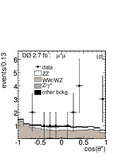
Figure 7: Distribution in the dimuon channel of the input variables of the likelihood discriminant for data and MC. $\chi^{2}$ probability for the kinematic fit to the dilepton mass (a), $p_{T}$ of the leading lepton (b), the opening angle between the lead lepton and the dilepton system(c), and the cosine of the scattering angle of the negative lepton in the dilepton rest frame (d).

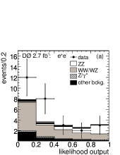
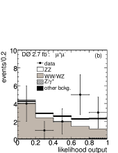
Figure 8: The likelihood distributions for signal and background: dielectron events (a) and dimuon events (b). All selection requirements have been applied.

VI Systematic Uncertainties

Systematic uncertainties are evaluated separately for the dielectron and the dimuon samples and for each of the data taking periods. The uncertainties affecting the overall scale factor of the MC cross sections are canceled out by normalizing to the data before the $\not\!\!E^{\prime}_{T}$ cut. The remaining systematic uncertainties contributing to the significance and cross section are dominated by the normalization of the $W$+jets background, the uncertainty on the $WW$ cross section, the lepton resolution, and the number of $Z$ events surviving the $\not\!\!E^{\prime}_{T}$ cut. The dominant uncertainties are listed in Table 3 in which $A_{Z}$ is the acceptance times efficiency for $Z/\gamma^{*}\rightarrow\ell^{+}\ell^{-}$ and $A_{ZZ}$ is the acceptance times efficiency for $ZZ/\gamma^{*}\rightarrow\ell^{+}\ell^{-}\nu\bar{\nu}$ where contributions from $Z/\gamma*\rightarrow\tau^{+}\tau^{-}$ decays are included. The large uncertainty on the $W$+jets and remaining $Z$ are due to the uncertainties on the jet to lepton misidentification rate used in the normalization of the $W$+jets background and the small statistics available after the $\not\!\!E^{\prime}_{T}$ cut (for both). Varying the parameters of the electron and muon smearing in the MC shows that the effect on the final result is within the statistical uncertainty in almost all bins. It is therefore propagated as an uncertainty in the shape of the likelihood, as are the contributions from jet energy resolution and the shape of the $ZZ\ p_{T}$ spectrum.

VII Cross Section and Significance

A negative log-likelihood ratio (LLR) test statistic is used to evaluate the significance of the result, taking as input the binned outputs of the dielectron and dimuon likelihood discriminants for each of the two data taking periods. A modified frequentist calculation is used b-collie which returns the probability of the background only fluctuating to give the observed yield or higher (p-value) and the corresponding Gaussian equivalent significance. The combined dielectron and dimuon channels yield an observed significance of $2.6$ standard deviations ($2.0$ expected), as reported in Table 4.

Because of the background normalization method described earlier, the measurement of the $ZZ\rightarrow\ell^{+}\ell^{-}\nu\bar{\nu}$ production cross section can be therefore expressed in terms of relative number of events with respect to the $Z\rightarrow\ell^{+}\ell^{-}$ sample.

We define a background hypothesis to include the distributions of the predicted backgrounds shown in Tables 1 and 2, and a signal hypothesis to include these backgrounds and the events from the $ZZ$ process.

To determine the cross section the likelihood distribution in the data has been fitted allowing the signal normalization to float. The scale factor $f$ with respect to the SM cross section and its uncertainty are determined by the fit. The ZZ production cross section is computed by scaling the number of events predicted by the MC to obtain that in data:

$$\sigma(ZZ)=\sigma(Z)\frac{A_{Z}}{A_{ZZ}}\frac{fN^{MC}_{ZZ}}{N_{Z}}$$

$A_{ZZ}$ is found to be $4.73\pm 0.03\%$ in the dielectron channel and $4.91\pm 0.03\%$ in the dimuon channel. We assume the theoretical cross section for $Z/\gamma^{*}\rightarrow\ell^{+}\ell^{-}$ in the mass window $60<M_{\ell\ell}<130$ GeV: $\sigma(Z)=256.6^{+5.1}_{-12.0}$ pb b-zxsec ; b-zxsec2 . Using the ratio of the $ZZ$ to $ZZ/\gamma^{*}$ cross sections computed with MCFM campbell-ellis at NLO, we scale the $ZZ/\gamma^{*}$ cross section down by 3.4% to give a pure $ZZ$ cross section. The resulting cross section for $p\overline{p}\rightarrow ZZ+X$ is

$$\sigma(ZZ)=2.01\pm 0.93(stat.)\pm 0.29(sys.)\ \mathrm{pb}.$$

This can be compared with the predicted SM cross section of $1.4\pm 0.1$ pb campbell-ellis at $\sqrt{s}=1.96$ TeV.

Table 3: The values assumed by the dominant systematic uncertainties for the various Monte Carlo signal and background samples in the dielectron and dimuon channels.

Systematic uncertainty	dielectron	dimuon
	(%)	(%)
$W$+Jets normalization	16	–
$WW$ and $WZ$
Theoretical cross sections	7	7
Number of $Z$ events surviving
the $\not\!\!E^{\prime}_{T}$ cut	18	3
Systematic uncertainty on the	Uncertainty
cross section	(%)
$Z/\gamma^{*}\rightarrow\ell^{+}\ell^{-}$
theoretical cross section	${}^{+2.0}_{-5.0}$	${}^{+2.0}_{-5.0}$
${A_{Z}}/{A_{ZZ}}$ ratio from pdf
uncertainties	1.8	1.8
${A_{Z}}/{A_{ZZ}}$ ratio from modeling
of the veto efficiency	0.8	0.8
${A_{Z}}/{A_{ZZ}}$ ratio from modeling
of the $ZZ$ $p_{T}$ spectrum	3.0	3.0

Table 4: Estimated significance for background only to fluctuate to at least the observed yield for the combined dielectron and dimuon channels in the two data taking periods.

	expected ($\sigma$)	observed ($\sigma$)
p-value	0.0244	0.0042
significance	2.0	2.6

VIII Conclusion

We performed a measurement of the production cross section of $ZZ\rightarrow\ell^{+}\ell^{-}\nu\bar{\nu}$ using 2.7 fb^-1 of data collected by the D0 experiment at a center of mass energy of 1.96 TeV. We observe a signal with a $2.6$ standard deviations significance ($2.0$ expected) and measure a cross section $\sigma(p\bar{p}\to ZZ)=2.01\pm 0.93\mathrm{(stat.)}\pm 0.29\mathrm{(sys.)}$ pb. This is in agreement with the standard model prediction of $1.4$ pb campbell-ellis .

We thank the staffs at Fermilab and collaborating institutions, and acknowledge support from the DOE and NSF (USA); CEA and CNRS/IN2P3 (France); FASI, Rosatom and RFBR (Russia); CNPq, FAPERJ, FAPESP and FUNDUNESP (Brazil); DAE and DST (India); Colciencias (Colombia); CONACyT (Mexico); KRF and KOSEF (Korea); CONICET and UBACyT (Argentina); FOM (The Netherlands); STFC (United Kingdom); MSMT and GACR (Czech Republic); CRC Program, CFI, NSERC and WestGrid Project (Canada); BMBF and DFG (Germany); SFI (Ireland); The Swedish Research Council (Sweden); CAS and CNSF (China); Alexander von Humboldt Foundation (Germany); and the Istituto Nazionale di Fisica Nucleare (Italy).

References

- (1) Visitor from Augustana College, Sioux Falls, SD, USA.
- (2) Visitor from The University of Liverpool, Liverpool, UK.
- (3) Visitor from INFN Torino, Torino, Italy.
- (4) Visitor from ECFM, Universidad Autonoma de Sinaloa, Culiacán, Mexico.
- (5) Visitor from II. Physikalisches Institut, Georg-August-University, Göttingen, Germany.
- (6) Visitor from Helsinki Institute of Physics, Helsinki, Finland.
- (7) Visitor from Universität Bern, Bern, Switzerland.
- (8) Visitor from Universität Zürich, Zürich, Switzerland.
- (9) Deceased.
- (10) R. Barate et al., (ALEPH Collaboration), Phys. Lett. B 469, 287 (1999); J. Abdallah et al., (DELPHI Collaboration), Eur. Phys. J C 30, 447 (2003); P. Achard et al., (L3 Collaboration), Phys. Lett. B 572, 133 (2003); G. Abbiendi et al., (OPAL Collaboration), Eur. Phys. J C 32, 393 (2004).
- (11) V. Abazov et al. (DØ Collaboration), Phys. Rev. Lett. 100, 131801 (2008).
- (12) T. Aaltonen et al., (CDF Collaboration), Phys. Rev. Lett. 100, 201801 (2008)
- (13) S. Abachi et al. (D0 Collaboration), Nucl. Instrum. Methods Phys. Res A 338, 185 (1994).
- (14) V.M. Abazov et al. (D0 Collaboration), Nucl. Instrum. Methods Phys. Res A 565, 463 (2006).
- (15) V.M. Abazov et al., Nucl. Instrum. Methods Phys. Res A 552, 372 (2005).
- (16) R. Brun and F. Carminati, CERN Program Library Long Writeup W5013 (1993).
- (17) V. Abazov et el. (DØ Collaboration), Phys. Rev. D 71, 072004 (2005); Erratum Phys. Rev. D 77, 039901(E) (2008).
- (18) G. Blazey et al. (DØ Collaboration), arXiv:hep-ex/0005012 (2000).
- (19) T. Sjöstrand et al., Comput. Phys. Commun. 135, 238 (2001) We used pythiaversion 6.409.
- (20) H.L. Lai et al., Phys. Rev. D 55, 1280 (1997).
- (21) V. Abazov et al. (DØ Collaboration), Phys. Rev. Lett. 100, 102002 (2008).
- (22) U. Baur, T. Han, and J. Ohnemus, Phys. Rev. D 57, 2823 (1998).
- (23) M.L. Mangano, M. Moretti, F. Piccinini, R. Pittau, and A. Polosa, J. High Energy Phys. 07, 001 (2003).
- (24) K. Ackerstaff et al. (OPAL Collaboration), Eur. Phys. J C4, 47 (1998).
- (25) W. Fisher, FERMILAB-TM-2386-E.
- (26) R. Hamberg, W.L. van Neerven and T. Matsuura, Nucl. Phys. B359, 343 (1991).
- (27) A.D. Martin, R.G. Roberts, W.J. Stirling, R.S. Thorne, Phys. Lett. B 604, 61 (2004).
- (28) J. M. Campbell and R.K. Ellis, Phy. Rev. D 60, 113006 (1999).