Simulations of the Sunyaev-Zeldovich Effect from Quasars

Abstract

Quasar feedback has most likely a substantial but only partially understood impact on the formation of structure in the universe. A potential direct probe of this feedback mechanism is the Sunyaev-Zeldovich effect: energy emitted from quasar heats the surrounding intergalactic medium and induce a distortion in the microwave background radiation passing through the region. Here we examine the formation of such hot quasar bubbles using a cosmological hydrodynamic simulation which includes a self-consistent treatment of black hole growth and associated feedback, along with radiative gas cooling and star formation. From this simulation, we construct microwave maps of the resulting Sunyaev-Zeldovich effect around black holes with a range of masses and redshifts. The size of the temperature distortion scales approximately with black hole mass and accretion rate, with a typical amplitude up to a few micro-Kelvin on angular scales around 10 arcseconds. We discuss prospects for the direct detection of this signal with current and future single-dish and interferometric observations, including ALMA and CCAT. These measurements will be challenging, but will allow us to characterize the evolution and growth of supermassive black holes and the role of their energy feedback on galaxy formation.

1 Introduction

The temperature fluctuations in the cosmic microwave background, as measured by the Wilkinson Microwave Anisotropy Probe (WMAP) satellite (Bennett et al. 2003) and numerous other microwave experiments (e.g., Dawson et al. 2002; Rajguru et al. 2005; Reichardt et al. 2008) have proven to be the single most powerful tool in constraining cosmology (Spergel et al. 2007). The temperature anisotropy has been mapped with large statistical significance on angular scales down to around a quarter degree, where the dominant physical mechanisms contributing to the fluctuations arise from density perturbations at the epoch of recombination. Attention is now turning to arcminute angular scales, where temperature fluctuations arise due to interaction of the microwave photons with matter in the low-redshift universe (for a brief review, see Kosowsky 2003). These low-redshift and small-angle anisotropies are collectively known as “secondary anisotropies” in the microwave background. The most prominent among them is the Sunyaev-Zeldovich (SZ) effect (Sunyaev & Zeldovich 1972) from the inverse Compton scattering of the microwave photons due to hot electrons. The SZ effect provides a powerful method for detecting accumulations of hot gas in the universe (Carlstrom Holder & Reese 2002). Galaxy clusters, which contain the majority of the thermal energy in the universe, provide the largest SZ signal; clusters were first detected this way through pioneering measurements over the past decade (e.g, Marshall et al. 2001) and thousands of them will be detected by the upcoming SZ surveys like the Atacama Cosmology Telescope (ACT) (Kosowsky et al. 2006) and the South Pole Telescope (SPT) (Ruhl et al. 2004). However, a number of other astrophysical processes will also create SZ distortions. This includes SZ distortion from peculiar velocities during reionization (McQuinn et al. 2005, Illiev et al. 2006), supernova-driven galactic winds (Majumdar, Nath, & Chiba 2001), black hole seeded proto-galaxies (Aghanim, Ballad & Silk 2000), kinetic SZ from Lyman Break Galaxy outflow (Babich & Loeb 2007), effervescent heating in groups and clusters of galaxies (Roychowdhury, Ruszkowski & Nath 2005) and supernova from first generation of stars (Oh, Cooray, & Kamionkowski 2003). The SZ distortion in galactic scales (hot proto galactic gas) have been studied by different authors (e.g, de Zotti et al. 2004, Rosa-Gonz’alez et al. 2004, Massardi et al. 2008 ). Here we investigate one generic class of SZ signals: the hot bubble surrounding a quasar powered by a supermassive black hole. Probing black hole energy feedback via SZ distortions is one direct observational route to understanding the growth and evolution of supermassive black holes and their role in structure formation. Analytic studies of this signal have been done by several authors (e.g., Natarajan & Sigurdsson 1999; Yamada, Sugiyama & Silk 1999; Lapi, Cavaliere & De Zotti 2003; Platania et al. 2002; Chatterjee & Kosowsky 2007); the current numerical work complements a similar study by Scannapieco Thacker and Couchman 2008.

Run	Boxsize	$N_{P}$	$m_{DM}$	$m_{gas}$	$\epsilon$	$z_{end}$
	($h^{-1}$ Mpc)		($h^{-1}M\odot$)	($h^{-1}M\odot$)	($h^{-1}$ kpc)
D4	33.75	$2\times 216^{3}$	$2.75\times 10^{8}$	$4.24\times 10^{7}$	6.25	0.00
D6 (BHCosmo)	33.75	$2\times 486^{3}$	$2.75\times 10^{7}$	$4.24\times 10^{6}$	2.73	1.00

Table 1: The numerical parameters in the simulation. For the current study we have used the low-resolution version because we have a matching simulation with no black holes; resolution effects are discussed in Sec. 4.3. $N_{p}$, $m_{DM}$, $m_{gas}$, $\epsilon$ and $z_{end}$ are defined as the total number of particles, mass of the dark matter particles, mass of the gas particles, gravitational softening length and final redshift run respectively.

Analytic models and numerical simulations of galaxy cluster formation indicate that the temperature and the X-ray luminosity relation should be related as $L_{x}\simeq T^{2}$ in the absence of gas cooling and heating (Peterson & Fabian 2006 and references therein). Observations show instead that $L_{x}\simeq T^{3}$ over the temperature range 2 to 8 kev with a wide dispersion at lower temperature, and a possible flattening above (Markevitch 1998; Arnaud & Evrard 1999; Peterson & Fabian 2006). The simplest explanation for this result is that the gas had an additional heating of 2 to 3 keV per particle (Wu, Fabian & Nulsen 2000; Voit et al. 2003). Several nongravitational heating sources have been discussed in this context (Peterson & Fabian 2006; Morandi Ettori & Moscardini 2007); quasar feedback (e.g., Binney & Tabor 1995; Silk & Rees 1998; Ciotti & Ostriker 2001; Nath & Roychowdhury 2002; Kaiser & Binney 2003; Nulsen et al. 2004) is perhaps the most realistic possibility. The effect of this feedback mechanism on different scales of structure formation have been addressed by several authors (e.g., Mo & Mao 2002; Oh & Benson 2003; Granato et al. 2004). The mechanism of quasar heating in cluster cores has been observationally motivated by studies from McNamara et al. 2005, Voit & Donahue 2005 and Sanderson, Ponman & O’Sullivan 2006 (see McNamara & Nulsen 2007 for a recent review). The impact of this nongravitational heating in galaxy groups, which have shallower potential wells and thus smaller intrinsic thermal energy than galaxy clusters, can also be substantial (Arnaud & Evrard 1999; Helsdon & Ponman 2000; Lapi, Cavaliere & Menci 2005). Observational efforts to detect the impact of this additional heating source in the context of quasar feedback have been carried out using galaxy groups in the Sloan Digital Sky Survey (SDSS) by Weinmann et al. 2006, and with a Chandra group sample by Sanderson, Ponman & O’Sullivan 2006. Detailed theoretical studies of galaxy groups using simulations which include quasar feedback have been undertaken by, e.g., Zanni et al. 2005, Sijacki et al. 2007, and Bhattacharya, Di Matteo & Kosowsky 2007. At smaller scales, the impact of quasar feedback has been investigated by Schawinski et al. 2007 with early-type galaxies in SDSS, and has also been studied in several theoretical models of galaxy evolution (e.g, Kawata & Gibson 2005; Bower et al. 2006; Cattaneo et al. 2007).

Growing observational evidence points to a close connection between the formation and evolution of galaxies, their central supermassive black holes (e.g., Magorrian et al. 1998, Ferrarese & Merritt 2000, Tremaine et al. 2002) and their host dark matter halos (Merritt & Ferrarese 2001; Tremaine et al. 2002). Several different groups have now investigated black hole growth and the effects of quasar feedback in the cosmological context (e.g., Scannapieco & Oh 2004; Di Matteo, Springel & Hernquist 2005; Lapi et al. 2006; Croton et al. 2006; Thacker, Scannapieco & Couchman 2006, Sijacki et al. 2007). Recently Di Matteo et al. (2008) carried out a hydrodynamic cosmological simulation following in detail the growth of supermassive black holes, using a simple but realistic model of gas accretion and associated feedback. Using this simulation, we construct maps of the SZ distortion around black holes of different masses at various redshifts. We demonstrate that the SZ signal around quasars scales with black hole mass and accretion rate. A similar approach has been taken by Scannapieco, Thacker & Couchman (2008) from a cosmological simulation with a different implementation of quasar feedback. Predictions for the SZ distortion due to a phenomenological treatment of galactic winds from simulations have been obtained previously by White, Hernquist & Springel (2002).

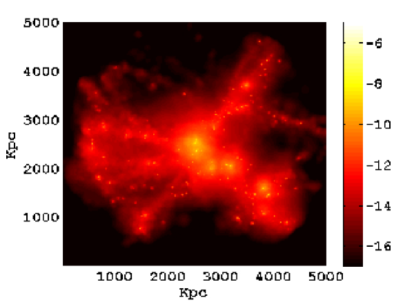
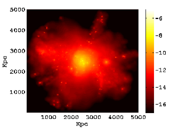
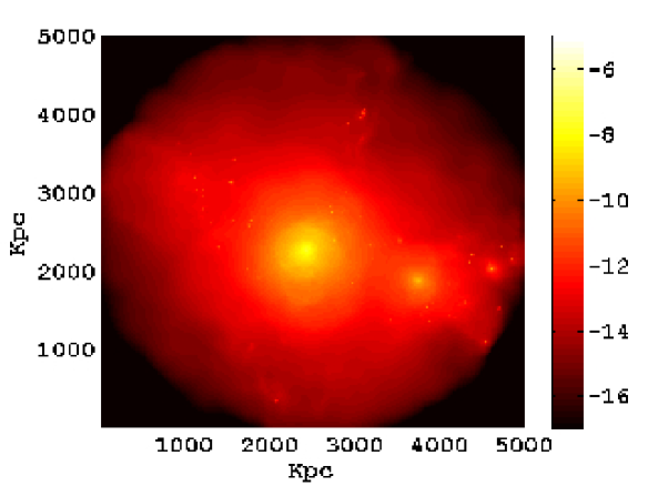
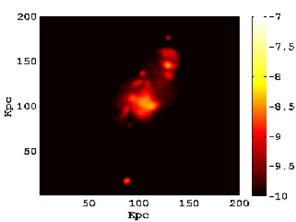
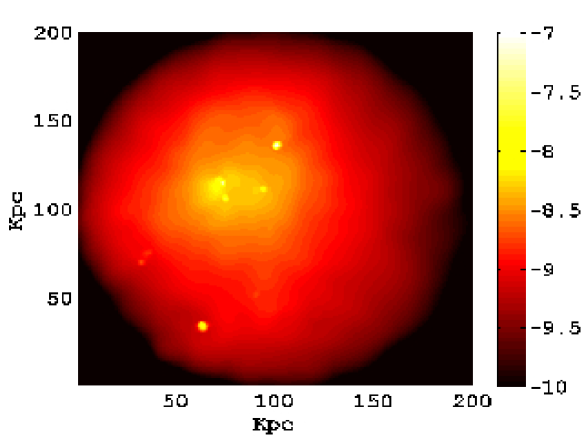
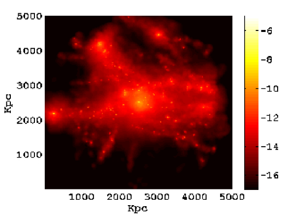
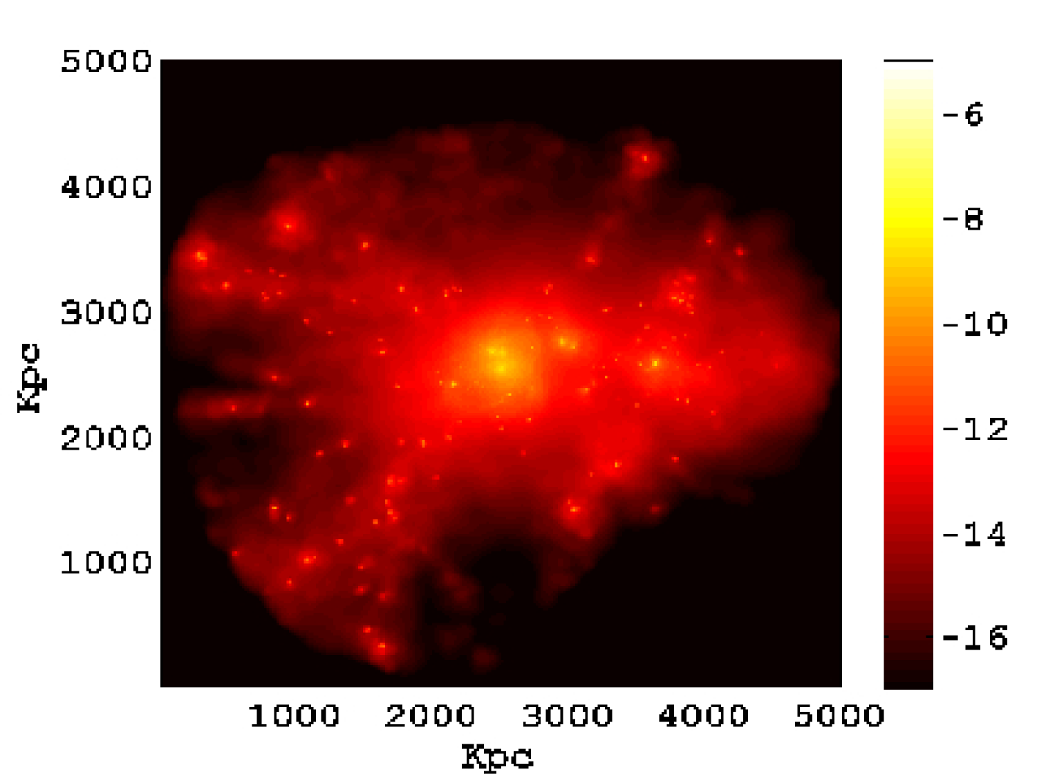
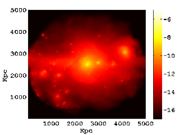
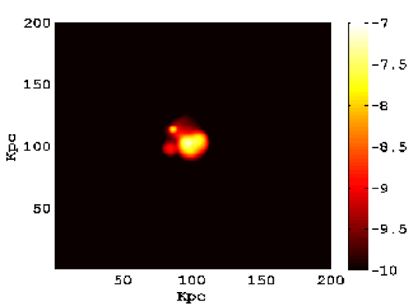
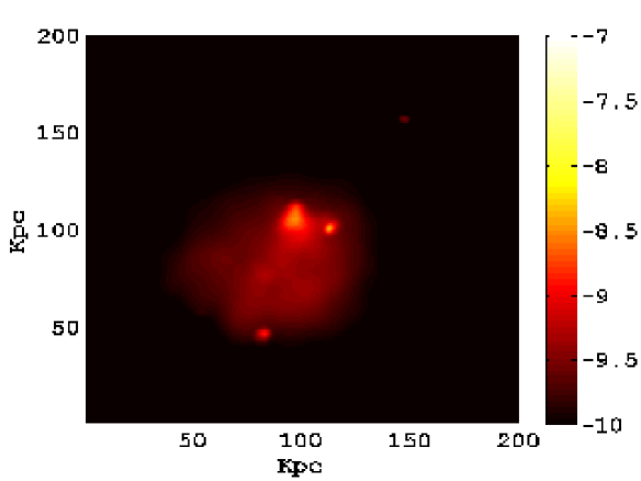
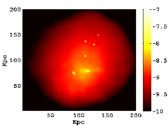
Figure 1: Simulated $y$-distortion maps around two massive black holes, at three different redshifts; left, middle, and right columns are for $z=3$, $z=2$, and $z=1$. The top two rows are for the most massive black hole in the simulation, with mass $7.35\times 10^{8}M_{\odot}$, $2.76\times 10^{9}M_{\odot}$ and $4.26\times 10^{9}M_{\odot}$ at redshifts 3, 2, and 1 respectively. The top row shows $y$ in a 5 Mpc square region centered on the black hole; the second row shows zooms in to a smaller region 200 kpc square. Note the two rows have different color scales. The third and fourth rows are the same as the first two rows, for a different black hole (the second most massive black hole at redshift 3.0) with mass $7.15\times 10^{8}M_{\odot}$, $8.2\times 10^{8}M_{\odot}$ and $2.11\times 10^{9}M_{\odot}$ at redshifts 3, 2, and 1. For both black holes, the peak value of $y$ is between $10^{-7}$ and $10^{-6}$, corresponding to an effective maximum temperature distortion between a few tenths of a $\mu$K to a few $\mu$K.

Typically, the SZ distortions from quasar feedback result in effective temperature distortions at the micro-Kelvin level on arcminute angular scales. Recent advances in millimeter-wave detector technology and the construction of several single-dish and interferometric experiments (see Birkinshaw & Lancaster 2007 for a recent review on SZ observations), including the Sub Millimeter Array (SMA), the combined array for research in Millimeter wave Astronomy (CARMA), the Cornell Caltech Atacama Telescope (CCAT), the Atacama Large Millimeter Array (ALMA), and the Large Millimeter Telescope (LMT), along with SZ surveys like ACT and SPT, have brought detection of this signal into the realm of possibility. Although the direct detection of this signal from current SZ surveys seems unlikely, since the amplitude of fluctuation observed is at or below the noise threshold of ACT or SPT (Chatterjee & Kosowsky 2007), proposed submillimeter facilities offer some possibility for direct detection of this signal. An additional route for detection is cross-correlation of optically-selected quasar with microwave maps (Chatterjee & Kosowsky 2007; Scannapieco Thacker & Couchman 2008). However, this approach likely requires multifrequency observations to discriminate the SZ effect from intrinsic quasar emission or infrared sources.

The paper is organized as follows. Section 2 describes the simulation that has been used in this work. In Section 3 we give a brief review of the SZ distortion and display the SZ maps derived from the simulation. Astrophysical results from the maps are presented in Section 4, including radial profiles around individual black holes and the correlation between black hole mass and SZ distortion. The concluding Section estimates detectability of these signals and summarizes future prospects. Throughout we use units with $c=k_{B}=1$.

	Most massive black hole			Second black hole
Redshift	$N_{BH}$	$dM/dt$, $M_{\odot}$/yr	Redshift	$N_{BH}$	$dM/dt$, $M_{\odot}$/yr
3.0	0	0.034	3.0	0	0.240
2.0	3	0.003	2.0	2	0.013
1.0	4	0.013	1.0	1	0.005

Table 2: The accretion rates and the number of neighboring black holes within a radius of 100 kpc, for the two black holes in Fig. 1.

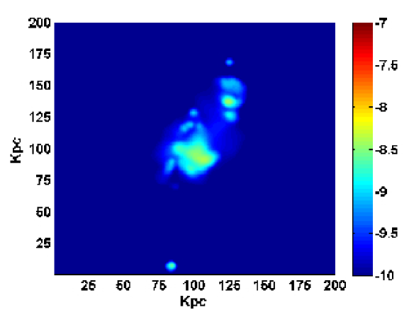
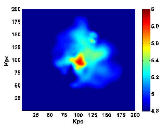
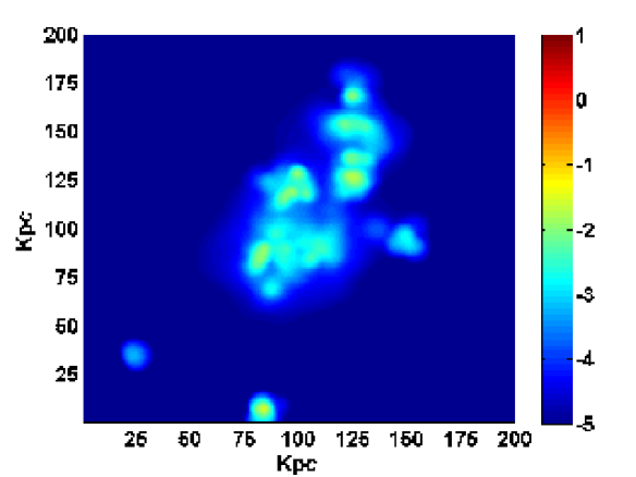
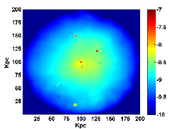
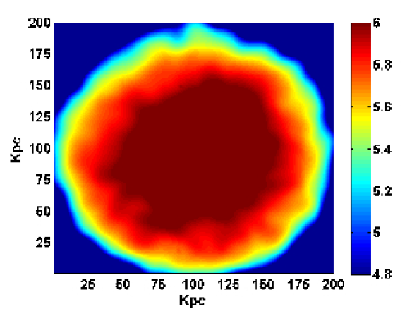
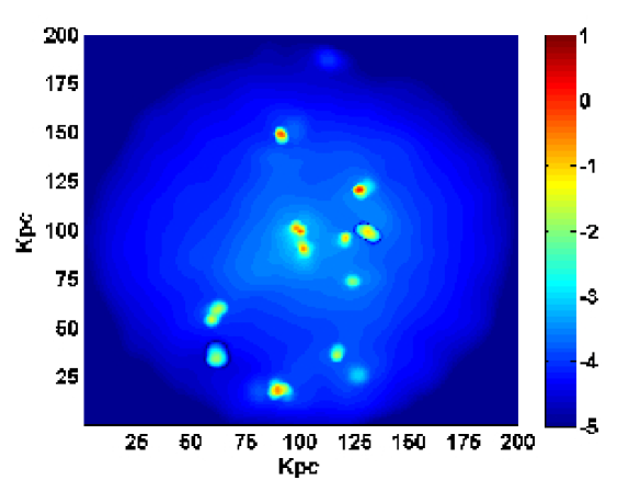
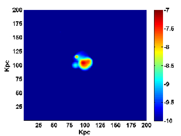
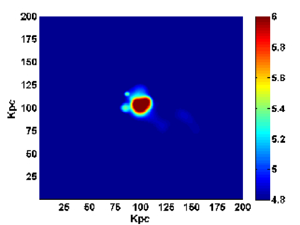
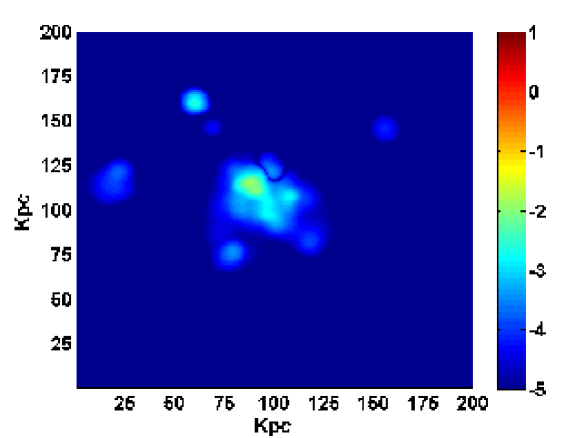
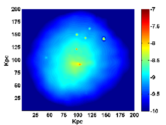
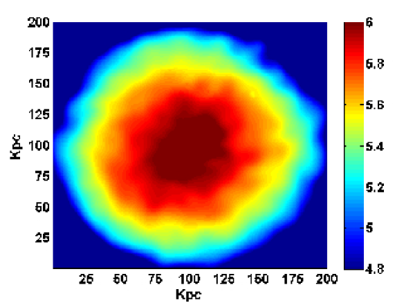
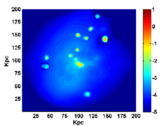
Figure 2: The difference in $y$-distortion between a simulation with black hole feedback and a simulation without, for the same region of space shown in Fig. 1. The two simulations have identical resolution and initial conditions. The first row corresponds to the most massive black hole at $z=3$, the second row at $z=1$; the third row corresponds to the other black hole (second most massive black hole at redshift 3.0) in Fig. 1 at $z=3$, the fourth row at $z=1$. The left column shows $y$, the middle shows the log of the mass-weighted average temperature in units of Kelvin. The right column shows the log of the electron number surface density in units of cm^-2 .

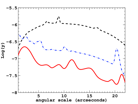
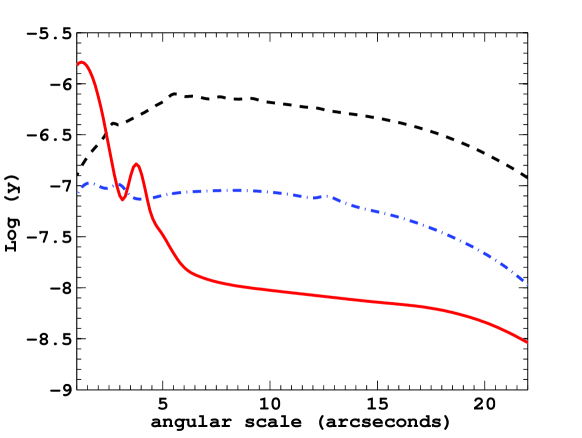
Figure 3: The angular profiles of the $y$ distortion for the two black holes shown in Fig. 1 at three different redshifts. The solid, dot-dashed and dashed lines are for redshifts 3, 2, and 1 respectively. The left panel shows the most massive black hole and the right panel is the other black hole (second most massive black hole at redshift 3.0). Although the central amplitude at a particular time depends strongly on the instantaneous state of the black hole accretion, the distortion amplitude increases monotonically with time at a 20 arcsecond angular distance.

2 Simulation

The numerical code uses a standard $\Lambda$CDM cosmological model with cosmological parameters from the first year WMAP results (Spergel et al. 2003). The cosmological parameters are $\Omega_{m}=0.3$, $\Omega_{\Lambda}=0.7$, $H_{0}=70$ km/s Mpc^-1 and Gaussian initial adiabatic density perturbations with a spectral index $n_{s}=1$ and normalization $\sigma_{8}=0.9$. (While the current lower value of $\sigma_{8}$ will affect the total number of black holes in a given volume, it should have little impact on the results for individual black holes presented here.) The simulation uses an extended version of the parallel cosmological Tree Particle Mesh-Smoothed Particle Hydrodynamics code GADGET2 (Springel 2005). Gas dynamics are modeled with Lagrangian smoothed particle hydrodynamics (SPH) (Monaghan 1992); radiative cooling and heating processes are computed from the prescription given by Katz, Weinberg, & Hernquist (1996). The relevant physics of star formation and the associated supernova feedback has been approximated based on a sub-resolution multiphase model for the interstellar medium developed by Springel & Hernquist (2003a).

A detailed description of the implementation of black hole accretion and the associated feedback model is given in Di Matteo et al. 2008. Black holes are represented as collisionless “sink” particles that can grow in mass by accreting gas or by merger events. The Bondi-Hoyle relation (Bondi 1952; Bondi & Hoyle 1944; Hoyle & Lyttleton 1939) is used to model the accretion rate of gas onto a black hole. The accretion rate is given by $\dot{M}_{BH}=4\pi[G^{2}M_{BH}^{2}\rho]/(c_{s}^{2}+v^{2})^{3/2}$, where $\rho$ and $c_{s}$ are density and speed of sound of the local gas, $v$ is the velocity of the black hole with respect to the gas, and $G$ is the gravitational constant. The radiated luminosity is taken to be $L_{r}=\eta(\dot{M}_{BH}c^{2})$ where $\eta=0.1$ is the canonical efficiency for thin disk accretion. It is assumed that a small fraction of the radiated luminosity couples to the surrounding gas as feedback energy $E_{f}$, such that $\dot{E_{f}}=\epsilon_{f}L_{T}$ with the feedback efficiency $\epsilon_{f}$ taken to be $5\%$. This feedback energy is put directly into the gas smoothing kernel at the position of the black hole (Di Matteo et. al 2008). The efficiency $\epsilon_{f}$ is the only free parameter in our quasar feedback model, and is chosen to reproduce the observed normalization of the $M_{BH}-\sigma$ relation (Di Matteo, Springel & Hernquist 2005). This number is also consistent with the preheating in groups and clusters that is required to explain their X-ray properties (Scannapieco & Oh 2004). The feedback energy is assumed to be distributed isotropically for the sake of simplicity; however the response of the gas can be anisotropic. This model of quasar feedback as isotropic thermal coupling to the surrounding gas is likely a good approximation to any physical feedback mechanism which leads to a shock front which isotropizes and becomes well mixed over physical scales smaller than those relevant to our simulations and on timescales smaller than the dynamical time of the galaxies (see Di Matteo et al. 2008 and Hopkins & Hernquist 2006 for more detailed discussions). In actual active galaxies, the accretion energy is often released anisotropically through jets. As radio galaxy lobes can have substantial separations, it is conceivable that actual hot gas bubble morphology could differ somewhat from that in the simulations. This difference needs to be investigated with further simulations, but the overall detectability of the signal depends primarily on its amplitude and characteristic angular scale, which are determined mainly by the total energy injection as a function of time. The results for the signals and detectability presented here are unlikely to differ significantly due to more detailed modeling of the energy injection morphology.

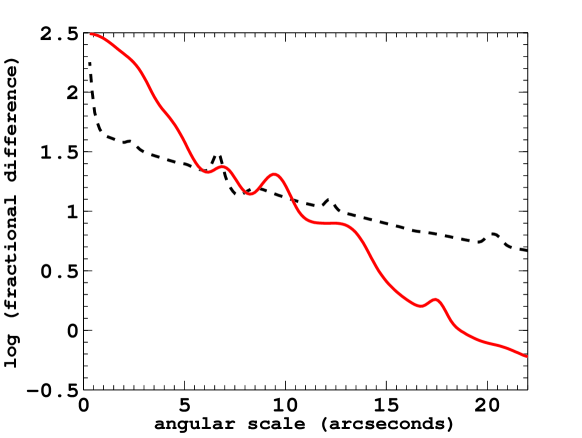
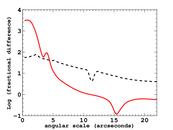
Figure 4: The difference in the $y$-distortion radial profile with and without black hole feedback, for the two black holes shown in Fig. 1. The left panel is for the most massive black hole and the right panel is for the second black hole (second most massive black hole at redshift 3.0). For each, the dashed line is the fractional change in the y distortion with respect to the no black hole case at $z=1$; the solid line is at $z=3$.

The formation mechanism for the seed black holes which evolve into the observed supermassive black holes today is not known. The simulation creates seed black holes in haloes which cross a specified mass threshold. At a given redshift, haloes are defined by a friends-of-friends group finder algorithm run on the fly. For any halo with mass $M>10^{10}h^{-1}M_{\odot}$ which does not contain a black hole, the densest gas particle is converted to a black hole of mass $M_{BH}=10^{5}h^{-1}M_{\odot}$; the black hole then grows via the accretion prescription given above and by efficient mergers with other black holes (Di Matteo et al. 2008). The simulations used in this paper have a box size of $33.75h^{-1}$ Mpc with periodic boundary conditions. The characteristics of the simulation are listed in Table 1, where $N_{p}$ is the total number of dark matter plus gas particles in the simulation, $m_{DM}$ and $m_{\rm gas}$ are their respective masses, $\epsilon$ gives the comoving softening length, and $z_{\rm end}$ is the final redshift of the run. For redshifts lower than 1, the fundamental mode in the box becomes nonlinear, so large-scale properties of the simulation are unreliable after $z=1$. The current results are derived for the D4 run with $2\times 216^{3}$ particles; we will present brief comparisons with the higher-resolution D6 (BHCosmo) run to demonstrate that our results are reasonably independent of resolution.

A different simulation and feedback model have recently been used by Scannapieco, Thacker & Couchman (2008) to study the same issues. They associate the remnant circular velocity within a post merger event with black hole mass. The time scale on which the black hole shines at its Eddington luminosity is assumed to be a fixed fraction of the dynamical time scale of the system; the time scale and black hole mass scale are used to estimate the energy output from a black hole. Their feedback energy efficiency into the intergalactic medium is 5%, consistent with the assumption in our simulation. In contrast, our simulation tracks the time-varying feedback from a given black hole due to changing local gas density as the surrounding cosmological structure evolves. This simulation offers the possibility of tracking the accretion history and duty cycle of black hole emission for individual black holes, which we plan to address in future work.

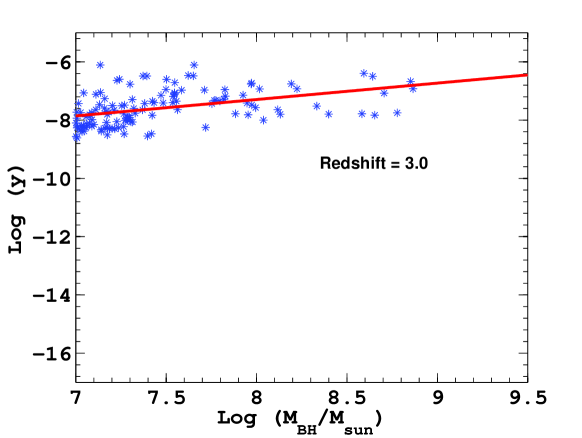
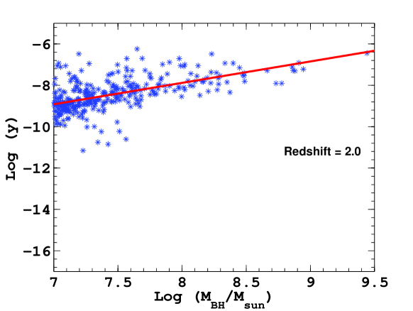
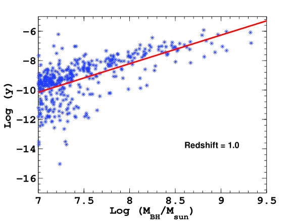
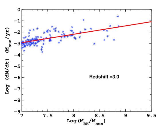
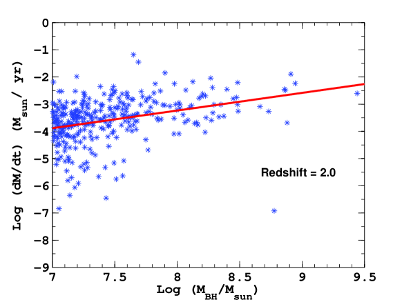
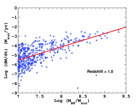
Figure 5: The top row shows the mean $y$ distortion within a comoving 200 kpc region around the black hole as a function of black hole mass, for redshifts 3,2,1 from left to right; at $z=1$ the angular size of the box is around 25 arcseconds. The bottom row shows the mass accretion rate as a function of black hole mass, for the same redshifts. The points are the numerical data and the solid lines are power-law fits. All black holes in the plotted mass range are included. The qualitative similarity between the top and the bottom panel shows the association of the $y$-distortion with accretion rates.

Redshift	$N_{BH}$	$N_{BH}$above $10^{7}M_{\odot}$	Fits for $y$	Fits for $dM_{BH}/dt$
3.0	2378	127	$\log y=0.56\log(M_{BH}/M_{\odot})-9.8$	$\log(dM_{BH}/dt)=0.74log(M_{BH}/M_{\odot})-8.1$
2.0	3110	336	$\log y=1.00\log(M_{BH}/M_{\odot})-14$	$\log(dM_{BH}/dt)=0.65logM_{BH}/M_{\odot})-8.4$
1.0	3404	404	$\log y=1.90\log(M_{BH}/M_{\odot})-22$	$\log(dM_{BH}/dt)=1.4log(M_{BH}/M_{\odot})-15$

Table 3: Numerical values used in Fig. 5. Column 2 shows the total number of black holes in the simulation at redshifts 3, 2, and 1, while column 3 shows the total number of black holes above a mass of $10^{7}M_{\odot}$. Columns 4 and 5 show the scaling relations displayed in Fig. 5. The mass accretion rate is in units of $M_{\odot}$/yr.

3 Results from the simulations

3.1 The Sunyaev-Zeldovich Distortion and Maps

The Compton $y$-parameter characterizing the non-relativistic thermal SZ spectral distortion is proportional to the line-of-sight integral of the electron pressure:

$$y=2\int dl\,\sigma_{T}n_{e}\frac{T_{e}}{m_{e}}$$ (1)

where $\sigma_{T}$ is the Thompson cross section, $n_{e}$ and $T_{e}$ are electron number density and temperature, and the integral is along the line of sight. The effective temperature distortion at a frequency $\nu$ is given by (Sunyaev & Zeldovich 1972)

$$\frac{\Delta T}{T_{0}}=\left[x\coth(x/2)-4\right]y,$$ (2)

where $x=h\nu/T_{0}$ and $T_{0}$ is the CMB temperature equal to 2.73 K.

Figure 1 shows $y$-distortion maps centered around two representative black holes in the simulation at redshifts 3, 2 and 1 (from left to right respectively). The two black holes are the most massive and the second most massive black hole at redshift 3.0 in the simulation. We have chosen the two most massive black holes in the simulation since the amplitude of the SZ distortion from the most massive black holes is relevent within the realm of current and future experiments. These maps were made by evaluating the line-of-sight integral in Eq. 1 through the appropriate portion of the simulation box. In order to characterize the large scale structure and associated $y$-distortions surrounding the black holes, we show a large region of the simulation within a comoving radius of 2.5 Mpc of the black hole in question, displayed with a comoving box size of 5 Mpc (top and third row for the most massive black hole and for another black hole in the simulation respectively) as well as a zoom into the central 200 kpc box (second and forth rows). The smaller region (200 Kpc) is the relevent scale of interest when looking at the direct impact of the central black hole to its surrounding gas; in the larger box multiple black holes are present. The mass of the central black hole is $7.35\times 10^{8}M_{\odot}$ at $z=3$, $2.76\times 10^{9}M_{\odot}$ at $z=2$, and $4.32\times 10^{9}M_{\odot}$ at $z=1$ (top two rows) and $7.11\times 10^{8}M_{\odot}$ at $z=3$, $8.2\times 10^{8}M_{\odot}$ at $z=2$, and $2.11\times 10^{9}M_{\odot}$ at $z=1$ (third and forth row). The feedback energy associated with black hole accretion creates a hot bubble of gas surrounding the black hole, which, as shown in the figures, grows significantly in size as redshift decreases. The growing hot bubble is roughly spherical by $z=1$, in agreement with the assumption of the analytic spherical blast wave model in Chatterjee and Kosowsky (2007).

In order to further characterize this expanding hot bubble, Fig. 2 displays maps of the difference between the two simulation with black hole modeling and without, in the same 200 kpc regions of Fig. 1. The top and second rows show the most massive black hole at $z=3$ and $1$ respectively while the third and forth row show the second black hole at the same redshifts. In this figure, the left column shows the logarithm of the $y$ distortion, the central column is the logarithm of the mass-weighted temperature in units of Kelvin and the right is the logarithm of projected electron number density in units of cm^-2,. At $z=3$ a residual $y$ distortion is evident and concentrated around the black hole, with little effect further out; the peak $y$ distortion due to the black hole is on the order of $10^{-7}$, corresponding to an effective temperature shift of the order of 1 $\mu$K. By $z=1$, the energy injected into the center has propagated outwards, forming a hot halo around the black hole. Table 2 shows the respective black hole accretion rates at different redshift for the two black holes in Figure 1 and 2. It is evident that the highest amplitude of $y$ distortion is associated with the most active, high-redshift epochs of accretion, when large amounts of energy are coupled to the surrounding gas via the feedback process. At $z=1$ the black hole accretion rate has dropped so the $y$ distortion has a smaller amplitude but has spread over a larger region (Fig. 2).

3.2 Angular Profiles

For the two black holes shown in Figure 1 we see an overall enhancement in the SZ signal due to quasar feedback. This agrees with the simulations in Scannapieco, Thacker & Couchman 2008. To further quantify the effects of quasar feedback we average the SZ signal in annuli around the black hole and examine the angular profile of the resulting $y$ from the hot bubble in Figure 3 and 4.

Figure 3 shows the average angular profiles of the total $y$ distortion around the two objects in the maps in Figure 1. The black dashed, blue dot-dashed and red solid lines are for $z=1$, $z=2$, and $z=3$ respectively. In both cases the $y$ increases with time between $\sim$ 10 to 25 arcsecond separation from the black hole. $y$ gets steadily larger as the feedback energy spreads over this volume (see also Fig.4). At $z=3$ the $y$ profile is steeper in the central regions with a significant peak (in particular for the second quasar) at scales below 5 arcseconds. The bumps in the profiles are due to concentrations of hot gas or occasional other black holes which are included in the total average signal. $y$ typically reaches its highest central peaks at time when the quasar is most active (the black hole accretion rate is high - see Table 2), and hence large amounts of energy are coupled to the surrounding gas according to our feedback prescription. For example, the $z=3$ curve in the right panel shows the black hole at a particularly active phase; the central $y$ distortion corresponds to a temperature difference of over 4 $\mu$K. At $z=2$ this central distortion is smaller by a factor of 20, while it is larger by a factor of 10 at an angular separation of 10 arcseconds. Figure 3 shows the total SZ effect in the direction of a quasar resulting from the superposition of the SZ signature from quasar feedback plus the SZ distortion from the rest of the line of sight due to the surrounding adiabatic gas compression, which is expected to form an average background level in the immediate vicinity of the back hole.

In order to clearly disentangle the contribution due to quasar feedback, in Figure 4, we plot the fractional change in $y$ distortion between the simulation with and without black hole modeling, at two different redshifts. These are the profiles corresponding to the maps shown in Figure 2. It is clear that the local SZ signature is largely dominated by the energy output from the black hole, giving a factor between 300 to over 3000 (for the second black hole at $z=3$ in right panel) increase in $y$ near the black hole. Our results are also consistent with the expected $y$ distortion from the thermalized gas in the host halos containing these black holes (which are on the order $10^{12}M_{\odot}$ to $10^{13}M_{\odot}$) and is the range $10^{-9}$ to $10^{-7}$ (see also Komatsu & Seljak 2002). The largest peak in $y$ distortion enhancement due to quasar feedback generally lies within 5 arcseconds of the black hole.

3.3 Black Hole Mass Scaling Relations

Since the SZ effect from the region around the black holes we analyzed in the previous section is dominated by the quasar feedback, we investigate whether a correlation between black hole mass and $y$ distortion exists for the population as a whole (see also Colberg & Di Matteo 2008 for other scaling relations between $M_{BH}$ and host properties). The top row of Figure 5 plots the mean $y$ distortion, computed over a sphere of radius 200 kpc/$h$ (i.e. the same as in the maps, corresponding to 20 arcseconds) versus black hole mass for all black holes in the simulations with $M_{BH}>10^{7}M_{\odot}$ at $z=1,2$ and $3$ (from right to left respectively). The size of the region is chosen to sample the entire region of distortion due to the quasar feedback, while minimizing bias from the local environment (Fig. 3 and 4). The mass cut-off is chosen to (a) minimize effects due to lack of appropriate resolution in the simulations as well as (b) produce SZ distortions that may be detectable by current or upcoming experiments.

Simple power law fits to the $y$ distortion as a function of black hole mass show a redshift evolution with the scaling becoming steeper with decreasing redshift. Table 3 summarizes our results from the fits. The trends show a close correspondence between the mean $y$ parameter and the total feedback energy as measured from $y$. In order to further investigate the reason for $y-M_{BH}$ relations, in the bottom row of Figure 5 we plot the accretion rate versus black hole mass at redshifts 3, 2, and 1 for the same sample as in the top panel and perform similar power-law fits (see Table 3). The trends in accretion rate versus $M_{BH}$ are qualitatively similar to the top panel, demonstrating the connection of the $y$ distortion due to quasar feedback with the black hole accretion rate and black hole mass. In particular, at $z=1$ the relations get steeper as expected if the largest fraction of black holes are accreting according to the Bondi scaling (e.g., $\dot{m}\propto M_{BH}^{2}$) and shallower with increasing redshift when most black holes are accreting close to the critical Eddington value (e.g., $\dot{m}\propto M_{BH}$). Of course, the accretion rate depends not only on black hole mass but also on the properties of the local gas and is also regulated by the large scale gas infall driven by major mergers, which peak at higher redshifts (Di Matteo et al. 2008). The ratio of the slopes (accretion rate to y distortion) for the fits shown in table 3 are 1.32, 0.65 and 0.73 at redshifts 3.0, 2.0 and 1.0 respectively. This shows the agreement of the top and the bottom panels in Figure 5, and the close connection between accretion history and SZ distortion: the SZ effect tracks closely quasar feedback and is promising probe of black hole accretion. The largest amplitudes of SZ signal from quasar is expected from $z\sim 2-3$ at a time close to the peak of the quasar phase in galaxies.

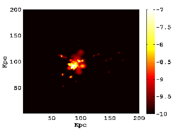
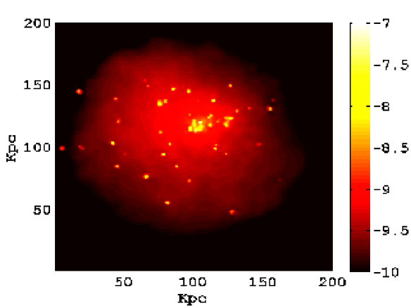
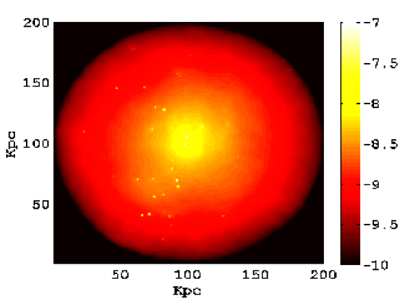
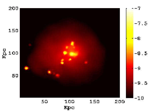
Figure 6: The top row shows $y$-distortion maps of the most massive black hole at $z=3$ (left), $z=2$ (center) and $z=1$ (right) in a higher-resolution (D6) simulation. The bottom row shows the same thing for a lower-resolution (D4) run. The black hole masses in the two simulations are slightly different from each other: for $z=1$ masses $4.29\times 10^{9}M_{\odot}$ (D4) and $2.96\times 10^{9}M_{\odot}$ (D6), for $z=2$ masses $2.76\times 10^{9}M_{\odot}$ (D4) and $1.83\times 10^{9}M_{\odot}$ (D6), and for $z=3$ masses $7.35\times 10^{8}M_{\odot}$ (D4) and $8.56\times 10^{8}M_{\odot}$ (D6). The box size is 200 kpc square. The difference in peak $y$ value for D4 and D6 varies from 22% ($z=3$) to 6% ($z=2$) and it is higher for the higher-resolution simulation at all three redshifts.

3.4 Resolution Test

In the previous section we have made use of the D4 (Table 1) simulations from our analysis. At this resolution we have two identical realizations, with and without black hole modeling, allowing us to carry out detailed comparisons of the effects of the quasar feedback. We now wish to assess possible effects due to numerical resolution by making use of the D6 (BHCosmo) run (see also Di Matteo et al. 2008, Croft et al. 2008 and Bhattacharya DiMatteo & Kosowsky 2008 for additional resolution studies). Figure 6 shows the $y$ distortion maps for the most massive black hole at redshifts 3, 2, and 1. The top row is for the higher-resolution BHCosmo run and the bottom row is for the lower-resolution run (D4). Our results at the lower resolution appear reasonably well converged, though with some differences. The central black hole masses in the two runs differ somewhat. At $z=1$, $2$, and $3$, the black hole masses in the D4 and BHCosmo run are ($4.29\times 10^{9}M_{\odot}$, $2.96\times 10^{9}M_{\odot}$), ($2.76\times 10^{9}M_{\odot}$, $1.85\times 10^{9}M_{\odot}$) and ($7.35\times 10^{8}M_{\odot}$, $8.56\times 10^{8}M_{\odot}$) respectively. It clear that the difference in resolution is affecting the black hole mass as expected from modest changes in mass accretion rate (which is sensitive to the gas properties close to the black hole). Also, more small scale structure in the gas distribution is evident at higher resolution, as expected. This affects the amplitude of the total SZ flux which is enhanced by about 6% at $z=2$ and by about 22% at $z=3$ (when it is most peaked around the black hole) in the higher resolution run.

4 Detectability and Discussion

Observationally, quasar feedback is directly detectable by resolving Sunyaev-Zeldovich peaks on small angular scales of tens of arcseconds with amplitudes of up to a few $\mu$K above the immediately surrounding region. The combination of angular scale and small amplitude make detecting this effect very challenging, at the margins of currently planned experiments. The necessary sensitivity requires large collecting areas, while the angular resolution needed points to an interferometer in a compact configuration, or a large single-dish experiment. Since the SZ signal is manifested as a peak over the surrounding background level, a region substantially larger than the SZ peak must be imaged. This requires a telescope having sufficient resolution to resolve the central peak in the SZ distortion in an SZ image and enough field of view so that the peak could be identified. An example is the compact ALMA subarray known as the Atacama Compact Array (ACA), composed of 12 7-meter dishes. The ALMA sensitivity calculator gives that the synthesized beam for this array is about 14 arcseconds, and the integration time required to attain 1 $\mu$K sensitivity per beam at a frequency of 145 GHz and a maximum band width of 16 GHz is on the order of 1000 hours (ALMA sensitivity calculator). A very deep survey with this instrument could detect the SZ effect from individual black holes. The 50-meter Large Millimeter-Wave Telescope instrumented with the AzTEC bolometer array detector will have a somewhat similar sensitivity but detectibility would require a very deep (thousands of hours) integration time. The Cornell-Caltech Atacama Telescope (CCAT), a 25-meter telescope, estimates a possible pixel sensitivity for SZ detection at 150 GHz of 310 $\mu{\rm K}\,{\rm s}^{1/2}$ for 26 arcsecond pixels, so a 30 hour observation could give 1$\mu$K pixel noise. These pixels would not be small enough to resolve the hot halo around a black hole, but might be able to detect the difference in a single pixel due to black hole emission compared to the surrounding pixels. Aside from raw sensitivity and angular resolution, a serious difficulty with direct detection is the confusion limit from infrared point source emission; these sources are generally high-redshift star forming galaxies with a high dust emission. CCAT estimates show that their one-source-per-beam confusion limit will be around 6 $\mu$K at 150 GHz (Golwala 2006). This will present substantial difficulties for detecting a 1 $\mu$K temperature distortion if accurate. It is noted that the observations in the sub-millimeter band is limited by confusion noise and so another possibility of direct detection of the signal through radio frequency telescopes could be considered. Massardi et al. 2008 shows that the confusion due to dusty galaxies is lower at 10 GHz then at 100 GHz. The authors show that for galactic scale SZ effect the optimal frequency range for detection is between 10 to 35 GHz. However substantial confusion from radio galaxies at these low frequency observations would still be a challenging issue in the direct detection of the signal.

Given these substantial difficulties associated with direct detection, an alternate route may be necessary. Cross-correlation of arcminute-resolution microwave maps with optically selected quasar or massive galaxies is a second possible detection strategy (Chatterjee and Kosowsky 2007, Scannapieco, Thacker, and Couchman 2008). By averaging over large numbers of objects, we can have an estimate of a small mean black hole distortion signal from the noise in the maps. The primary challenge with this technique is the direct emission from quasar in the microwave band. It may be possible to select a sample of quasar which is sufficiently radio-quiet that the cross-correlation is not dominated by the intrinsic emission. Another possibility is to select massive field galaxies under the assumption that they harbor a central massive black hole which at one time was active; the hot bubble produced has a cooling time comparable to the Hubble time, so formerly active galaxies should still have an SZ signature. Finally, the SZ effect from black holes is in addition to the SZ emission from any hot gas in which the black hole’s host galaxy is embedded. Massive galaxies trace large-scale structure, and any cross-correlation will also detect this signal. Although the observational requirements for the cross-correlation method are plausible the scopes for detectibility with this method is still limited by confusion noise. Stacking microwave (SZ) maps in the direction of known quasars would also serve as an independent route in detecting the signal (Chatterjee & Kosowsky 2007). This can improve the signal to noise by a substantial amount although this method would still be limited by the uncertainties described above. Quantifying in detail the observable signal (which will need to be disentangled from other confusions such as dusty galaxies, radio galaxies etc.) for the possible direct detections methods or from cross-correlation analysis that we have discussed is beyond the scope of this paper and we defer it to a future work. The simulations and maps presented here provide a basis for further modeling of all these effects.

The main conclusions drawn from this work are summarized as follows. We have used the first cosmological simulations to incorporate realistic black hole growth and feedback to produce simulated maps of the Sunyaev-Zeldovich distortion of the microwave background due to the feedback energy from accretion onto supermassive black holes. These simulations address the rapid accretion phases of black holes: periods of strong emission are typically short-lived and require galaxy mergers to produce strong gravitational tidal forcing necessary for sufficient nuclear gas inflow rates (Hopkins, Narayan & Hernquist 2006; Di Matteo et al. 2008). The result is heating of the gas surrounding the black hole, so that the largest black holes produce a surrounding hot region which induces a $y$-distortion (related to a temperature distortion) with a characteristic amplitude of a few $\mu$K. We have obtained a scaling relation between the black hole mass and their SZ temperature decrement, which in turn is a measure of the amount of feedback energy output. The correspondence between the y distortion and the accretion rates is not exact but there is a close association which shows the correlation between feedback output and black hole activity. From our results we have shown that with the turn on of AGN feedback the signal gets enhanced largely and the enhancement is predominant at angular scales of 5 arcseconds. Finally we have shown that there is a fair probability of detecting this signal even from the planned sub millimeter missions.

The role of energy feedback from quasars and from star formation is known to have substantial impact on the process of galaxy formation and evolution of the intergalactic medium, but the details of this process are not well understood. Probes based on Sunyaev-Zeldovich distortions are challenging, but an eventual detection can be used to put useful constraints and checks on models of AGN feedback.

5 acknowledgments

SC would like to thank Bruce Partridge and James Moran for helpful discussions on experimental capabilities of various telescopes. Special thanks to Mark Gurwell for helping with the sensitivity calculation for SMA. SC and AK would also like to thank Christoph Pfrommer for some initial discussions on the project. Thanks to Jonathan Las Fargeas who helped with the analysis, supported by NSF grant 0649184 to the University of Pittsburgh REU program. We would also like to thank the referee for valuable suggestions on improvement of the paper.This work was supported at the University of Pittsburgh by the National Science Foundation through grant AST-0408698 to the ACT project, and by grant AST-0546035. At CMU this work has been supported in part through NSF AST 06-07819 and NSF OCI 0749212. SC was also partly funded by the Zaccheus Daniel Fellowship at the University of Pittsburgh.

References

- (1) Aghanim N., Balland, C., & Silk, J. 2000, A&A, 357, 1
- (2) Arnaud M., & Evrard A. E., 1999, MNRAS, 305, 631
- (3) Babich, D. & Loeb, A. 2007, MNRAS, 374, L24
- (4) Bennett et al., 2003, ApJs, 148, 1
- (5) Bhattacharya S., Di Matteo T., & Kosowsky A., 2007, ArXiv e-prints, 710, arxiv:07105574
- (6) Binney J., & Tabor G., 1995, MNRAS, 276, 663
- (7) Birkinshaw M., & Lancaster K., 2007, NewAR, 51, 346
- (8) Bondi H., 1952, MNRAS, 112, 195
- (9) Bondi H., & Hoyle F., 1944, MNRAS, 104, 273
- (10) Bower R. G., Benson A. J., Mallbon R., Helly J.C., Frenk C. S., Baugh C. M., Cole S., & Lacey C. G., 2006, MNRAS, 370, 645
- (11) Carlstrom J., E., Holder, G., P., & Reese, E. D., 2002, ARA&A, 40, 643
- (12) Cattaneo A. et al., 2007, MNRAS, 377, 63
- (13) Chatterjee S., & Kosowsky A., 2007, ApJL, 661, L113
- (14) Ciotti L., & Ostriker J. P., 2001, 551, 131
- (15) Colberg J. & Di Matteo T., 2008, MNRAS, in press
- (16) Croft R.A.C., Di Matteo T., Springel, V., Hernquist, L., 2008, MNRAS, submitted
- (17) Croton D. et al., 2006, MNRAS, 365, 11
- (18) Dawson K. S. et al., 2002 ApJ, 581, 86
- (19) De Zotti G., Burigana C., Cavaliere A., Danese L., Granato G. L., Lapi, A., Platania, P., & Silva, L., 2004, AIPC, 703, 375D
- (20) Di Matteo T., Springel V., & Hernquist L., 2005, Nature, 433, 604
- (21) Di Matteo T., Colberg J., Springel V., Hernquist L., & Sijacki D., 2008, ApJ, 676, 33
- (22) Ferrarese L., & Merritt D., 2000, ApJ, 539, L9
- (23) Golwala S., 2006, http://www.astro.caltech.edu/golwala/talks /CCATFeasibilityStudySZScience.pdf
- (24) Granato G. L., De Zotti G., Silva, L., Bressan A., & Danese L., 2004, ApJ, 600, 580
- (25) Helsdon S. F., & Ponman T. J., 2000, MNRAS, 315, 356
- (26) Hopkins P F., Hernquist L., 2006, ApJS, 163, 50
- (27) Hopkins P F., Narayan R., & Hernquist L., 2006, ApJ, 643, 641
- (28) Hoyle F., & Lyttleton R. A., 1939, in proceedings of the Cambridge Philosophical Society, 405
- (29) Iliev, I. T., Pen, U.-L., Bond, J. R., Mellema, G., & Shapiro, P. R. 2006, New Astron. Rev. 50, 909.
- (30) Kaiser C. R., & Binney J. J., 2003, MNRAS, 338, 837
- (31) Katz N., Weinberg D. H., & Hernquist L., 1996, ApJS, 105, 19
- (32) Kawata D., & Gibson B. K., 2005, MNRAS, 358, L16
- (33) Komatsu E., & Seljak U., 2002, MNRAS, 336, 1256
- (34) Kosowsky A., 2003, AIP Conf. Proc. 666, 325.
- (35) Kosowsky A. et al., 2006, New Astron. Rev. 50, 969.
- (36) Lapi A., Cavaliere A., & De Zotti G., 2003, ApJl, 597, L93
- (37) Lapi A., Cavaliere A., & Menci N., 2005, ApJ, 619, 60
- (38) Lapi A., Shankar F., Mao J., Granato G. L., Silva L., De Zotti G., & Danese L., 2006, ApJ, 650, 42
- (39) Magorrian, J., et al., 1998, AJ, 115, 2285
- (40) Majumdar, S. Nath, B., & Chiba, M. 2001, MNRAS, 324, 537
- (41) Markevitch M., 1998, ApJ, 504, 27
- (42) Marshall et al. 2001, ApJ, 551, L1-L4
- (43) Massardi M., Lapi A., de Zotti G., Ekers R. D., & Danese L., 2008, MNRAS, 384, 701
- (44) McNamara B. R., Nulsen P. E. J., Wise M. W., Rafferty D. A., Carilli C., Sarazin C. l., & Blanton E. L., 2005, Nature, 433, 45
- (45) McNamara B. R., & Nulsen P. E. J., 2007, ARA&A, 45, 117
- (46) McQuinn, M., Furlanetto, S. R., Hernquist, L., Zahn, O., & Zaldarriaga, M. 2005, ApJ, 630, 643
- (47) Merritt D., & Ferrarese L., 2001, ApJ, 547, 140
- (48) Mo H. J., & Mao S., 2002, MNRAS, 333, 768
- (49) Morandi A., Ettori S., & Moscardini L., 2007, MNRAS, 379, 518
- (50) Monaghan J. J., 1992, ARA&A, 30, 543
- (51) Natarajan P., & Sigurdsson S., 1999, MNRAS, 302, 288
- (52) Nath B. B., & Roychowdhury S., 2002, MNRAS, 333, 145
- (53) Nulsen P., Mcnamara B., David L., & Wise M., 2004, cosp, 35, 3235
- (54) Oh S. P., & Benson A., 2003, MNRAS, 342, 664
- (55) Oh, S. P., Cooray, A., & Kamionkowski, M. 2003, MNRAS, 342, 20
- (56) Peterson R., & Fabian A., 2006, Phys. Rep., 427, 1
- (57) Platania P., Burigana C., De Zotti G., Lazzaro E., & Bersanelli M., 2002, MNRAS, 337, 242
- (58) Reichardt et al., 2008, Arxiv e-prints, 801, arxiv:08011491
- (59) Rajguru et al., 2005, MNRAS, 363, 1125
- (60) Rosa-Gonzalez D., Terlvich R., Terlvich E., Friaca A., & Gaztanaga E., 2004, MNRAS, 348, 669
- (61) Roychowdhury S., Ruszkowski, M., & Nath, B. B. 2005, ApJ, 634, 90
- (62) Ruhl J. E. et al., 2004, Proc. SPIE, 5498, 11
- (63) Sanderson A. J. R., Ponman T. J., & O’Sullivan E., 2006, MNRAS, 372, 1496
- (64) Scannapieco E., & Oh S. P., 2004, ApJ, 608, 62
- (65) Scannapieco E., Thacker R. J., Couchman H. M. P., 2008, ApJ, 678, 674
- (66) Schawinski K., Tomas D., Sarzi M., Maraston C., Kaviraj S., Joo S., Yi S., Silk J., 2007, ArXiv e-prints, 709, arXiv:0709.3015
- (67) Sijacki D., Springel V., DiMatteo T., & Hernquist L., 2007, MNRAS, 380, 877
- (68) Silk J., & Rees M. J., 1998, A&A, 331, L1
- (69) Spergel D. N. et al., 2003, ApJS, 148, 175
- (70) Spergel D. N. et al., 2007, ApJS, 170, 377
- (71) Springel V., 2005, MNRAS, 364, 1105
- (72) Springel V., & Hernquist L., 2003a, MNRAS, 339, 312
- (73) Sunyaev R. A., & Zel’dovich Ya. B., 1972, Comments Astrophys. Space Phys., 4, 173
- (74) Thacker R. J., Scannapieco E., & Couchman H. M. P., 2006, ApJ, 653, 86
- (75) Tremaine, S. et.al. 2002, ApJ, 574, 740
- (76) Voit G. M., Balogh M. L., Bower R. G., Lacey C. G., & Bryan G. L., 2003, ApJ, 593, 272
- (77) Voit G. M., & Donahue M., 2005, ApJ, 634, 955
- (78) Weinmann S. M., vandenBosch F. C., Yang X., Mo H. J., Croton D. J., & Moore B., 2006, MNRAS, 372, 1161
- (79) White M., Hernquist L., Springel V., 2002, ApJ, 579, 16
- (80) Wu K. K. S., Fabian A. C., & Nulsen P. E. J., 2000, MNRAS, 318, 889
- (81) Yamada M., Sugiyama N., & Silk J. 1999, ApJ, 522, 66
- (82) Zanni C., Murante G., Bodo G., Massaglia S., Rossi P., & Ferrari A., 2005, A&A, 429, 399