VOSA: Virtual Observatory SED Analyzer.

Abstract

Context. The physical properties of almost any kind of astronomical object can be derived by fitting synthetic spectra or photometry extracted from theoretical models to observational data.

Aims. We want to develop an automatic procedure to perform this kind of fittings to a relatively large sample of members of a stellar association and apply this methodology to the case of Collinder 69.

Methods. We combine the multiwavelength data of our sources and follow a work-flow to derive the physical parameters of the sources. The key step of the work-flow is performed by a new VO-tool, VOSA. All the steps in this process are done in a VO environment.

Results. We present this new tool, and provide physical parameters such as T_eff, gravity, luminosity, etc. for $\sim$170 candidate members to Collinder 69, and an upper-limit for the age of this stellar association.

Conclusions. This kind of studies of star forming regions, clusters, etc. produces a huge amount of data, very tedious to analyse using the traditional methodology. Thus, they are excellent examples where to apply the VO capabilities.

1 Introduction

The determination of physical parameters of astronomical objects from observational data is frequently linked with the use of theoretical models as templates. In the case of stars, it is very common to estimate gravities by fitting different model/templates to gravity–sensitive lines (and other features, Decin et al. 2004) within the wavelength coverage of the observed spectra. Another method in the same framework is the comparison of the shape of the Spectral Energy Distributions (SEDs hereafter) constructed from observational photometric data with the corresponding synthetic ones derived using large grids of theoretical spectra (see for example Robitaille et al. 2007).

The use, -in the traditional way-, of these methodologies can easily become tedious and even unfeasible when applied to large amount of data. Nowadays, astronomers deal with very large databases, including not only empirical/observational entries, but also theoretical ones (for instance, models from different groups that need to be combined in order to reproduce the observations).

The Virtual Observatory (VO) philosophy (see Section 3) seems to be a reasonable approach to solve some intrinsic problems generated by this new way of working in astronomy. VO-tools now allow astronomers to deal with their own observational or theoretical databases and compare them (in an efficient way) with others already published in the “on-line literature”.

Here we present a work-flow to estimate the effective temperature (T_eff), gravity and luminosity (and, when comparing with theoretical isochrones and evolutionary tracks, age and mass) of members of an stellar association (in this particular case, Collinder 69, Barrado y Navascués et al. 2004b) based on their photometry. This work-flow has been built mainly with steps that are “VO-compliant”.

In Section 2 we explain the scientific case that caused the development of VOSA, the key VO-tool used in this work-flow. In Section 3 we describe the philosophy of the Virtual Observatory and some of its most known applications (tools that we have used in several steps of the process). In that section we also explain all the capabilities of the previously mentioned VO-tool VOSA (developed by the Spanish Virtual Observatory specially for this work). In Section 4 we explain step by step the work-flow followed to determine the physical parameters and properties of our sources. In Sections  5 and  6, we present the results and conclusions of this work, respectively. Finally, in Appendix A, we focus on technical issues concerning the computation of synthetic photometry and in Appendix B we provide a graphical scheme of the work-flow.

2 The scientific case

One of the most interesting Star Forming Regions (SFR) is associated to the O8III star $\lambda$ Orionis (located at about 400 pc from the Sun, and presenting very low extinction in its inner area, a central ring where A${}_{V}\sim 0.36$ magnitudes). This star dominates the eponymous cluster (also designated as Collinder 69), with an age of about 5 Myr (Dolan & Mathieu 1999, 2001; Barrado y Navascués et al. 2004b).

The $\lambda$ Orionis SFR includes several distinct associations apart from Collinder 69 (as Barnard 30, Barnard 35, and dark clouds like LDN 1588 and 1603). But, for this work, we will focus on the central cluster. Our goal is to determine physical parameters and properties (such as T_eff, bolometric luminosity, mass and age) of $\sim$ 170 candidate members of this cluster by comparing their SEDs with theoretical models.

Studying the physical parameters of a large population of sources belonging to the same cluster is advantageous, since we can infer properties not only of the individual sources but also of the association as a whole, for example its age, since we can assume that all objects are coeval. In this work we want to derive these physical parameters and properties by comparing observed SEDs with theoretical data; therefore, as a first step, we need to compile all the photometric/spectral information available for each of our sources in order to be able to decide which model reproduces best the observed data.

On the other hand, there are different collections of models (translated in thousands of individual models) that we might want to compare to the observations.

Trying to compile all the information available for each object and then compare the built SED with all the available models one by one with classical methodologies can be very tedious and time consuming, therefore we need to automatise the process as much as possible.

3 The VO–tools

The Virtual Observatory (IVOA) is an international, community-based initiative to provide seamless access to the data available from astronomical archives and services as well as state-of-the-art tools for the efficient analysis of this huge amount of information. The works by Padovani et al. (2004) and Tsalmantza et al. (2006) are good examples of the efficiency of such tools in helping astronomers to produce scientific results.

3.1 General-purpose tools

In this work we have taken advantage of the capabilities of Aladin, an interactive sky atlas developed by CDS that allows the user to visualise and analyse astronomical images, spectra and catalogues available from the VO services. We have also used TOPCAT, an interactive graphical viewer and editor for tabular data as well as different tools for analysing astronomical spectra (VOSED, VOSpec, SPECVIEW and SPLAT).

Regarding the data format, we have used the standard tabular format of the VO environment, the VOTable, whenever possible.

3.2 VOSA

As mentioned in the Introduction, a new VO-tool has been developed by the Spanish Virtual Observatory for the scientific case discussed in Section 2. This tool has been named VOSA (Virtual Observatory SED Analyzer), and can be accessed through its web-base interface at:
http://www.laeff.inta.es/svo/theory/vosa/

In order to use VOSA, the user only has to register in the service and start working. The system is based on sessions that can be saved, so that the user can recover the files and results obtained in a previous session (without redoing the fit process) and compare those results with new approaches (models, parameters, etc.). These sessions will remain in the system unless there is no activity in seven days (in that case the session will be erased).

VOSA performs the following tasks:

1. Read user photometry-tables.

   The input file can be either an ASCII table or a VOTable but with a specific format consisting of eight columns/fields as follows:

   Source Identifier: this will be used, for instance, as the title of the plots of the fittings.

   Coordinates of the source: Right ascension and Declination (in J2000) will be used to look for counterparts in various catalogs.

   Distance to the source in parsecs: this datum is mandatory in order to estimate the bolometric luminosity of the source. Should this parameter be unknown then type in a value of “$---$” and a generic distance of 10 parsecs will be assumed.

   Visual extincion (A_V in magnitudes) affecting the source: this value is used to deredden each SED (the Indebetouw et al. 2005 extinction law is applied).

   Filter name: a list of the already available filters can be found in the Help menu, new filters can be included upon user request.

   Observed flux/magnitude (flux in units of erg/cm²/s/Å).

   Flux/magnitude error (same units as in the previous field).

   For an example of the data ingestion interface see Fig. 9 in Appendix B. A more detailed description of the file format, available filters, fluxes for zero magnitude, etc. can be accessed from the VOSA Help menu.

2. Query several photometric catalogs accessible through VO services in order to increase the wavelength coverage of the data to be analised. Nowadays the user can query the 2MASS All-Sky Point Source Catalog (Skrutskie et al. 2006), the Tycho-2 Catalog (Høg et al. 2000), and the Strömgren uvby-beta Catalog (Hauck & Mermilliod 1998) using different radii according to the astrometic precision of each catalog.

3. Query VO-compliant theoretical models (spectra) for a given range of physical parameters.

   The user can choose among the different available collections of models (in a future implementation of the tool, it will offer the possibility to access any VO-compliant theoretical model collection). These models are accessible in a VO-environment from the SVO theoretical data server at http://laeff.inta.es/svo/theory/db2vo/

4. Calculate the synthetic photometry of the theoretical spectra (within the range of physical parameters required by the user) for the set of filters used to obtain the observed data (including the dataset coming from the VO photometrical services).

   The synthetic photometry is calculated by convolving the filter response curve with the synthetic spectra. Prior to this, both, the response curve and the synthetic spectra, are interpolated to match the spectral resolution; besides, the area of the response curve is normalised to unity to provide the user with a flux density that can be directly compared with the observed one (see Appendix A for the formal description of the process).

   Since some of the response curves for the set of filters that we use in our scientific case (for example the four channels of Spitzer/IRAC, Fazio et al. 2004, and the 24 micron channel of Spitzer/MIPS, Rieke et al. 2004) were not available in the VO Filter Profile Service, we consulted directly the web pages of the respective consortia and included them in VOSA (the transmission curves can be visualised and downloaded from the Help menu).

5. Perform a statistical test to decide which set of synthetic photometry reproduces best the observed data.

   The provided “best” fitting model is the one that minimises the value of the reduced $\chi^{2}$ defined as:

   $$\chi^{2}=\frac{1}{N-P}\sum\left\{\frac{1}{\sigma_{0}^{2}}(Y_{0}-M_{\rm d}\times Y_{\rm m})^{2}\right\}$$ (1)

   where $Y_{0}$ is the observed flux, $\sigma_{0}$ the observational error in the flux, $N$ the number of photometric points, $P$ the number of parameters being fitted, $Y_{\rm m}$ the theoretical flux predicted by the model and $M_{d}$ the multiplicative dilution factor, defined as $(R/D)^{2}$ (for models from Hauschildt et al. 1999; Allard et al. 2001 and Chabrier et al. 2000), $R$ being the radius of the source and $D$ the distance to the object.

   During the fitting process, the tool detects possible infrared excesses (in our scientific case some of the sources might be surrounded by disks). Thus, since the theoretical spectra correspond to stellar atmospheres, for the calculation of the $\chi^{2}$ the tool only considers those data points of the SED corresponding to bluer wavelengths than the one where the excess has been flagged.

   The excesses are detected by calculating iteratively (adding a new data point from the SED at a time), in the mid-infrared (wavelengths redder than 2.5$\mu$m), the $\alpha$ parameter as defined in Lada et al. (2006) (which becomes larger than -2.56 when the source present an infrared excess). The last wavelength considered in the fitting process together with the ratio between the total number of points belonging to the SED to those really used are displayed in the result tables.

   Once the fitting process is completed, the tool allows the user to check whether any other of the five “best” fits, per collection of models (meaning 20 best fits when using the four collections of models available in the server nowadays), turns out to be more convincing for him/her than the one that minimises the $\chi^{2}$ and choose that one as the best model to include in the final results table. For instance, the user might have a more accurate estimation of the gravity, which is important since changes in the surface gravity of stellar and sub-stellar sources do not produce dramatic differences in the shape of their SEDs.

6. Use the best-fit model as the source of a bolometric correction.

   The best fitting model is used to infer the total observed flux for each source of the sample ; this process is performed by integrating the total observed flux (where no excess has been detected), and using the best fitting model to infer that flux in the wavelength range where no observational data is available or some infrared excess has been detected (see Appendix A for a formal description of the procedure). We note that if the model reproduces the data correctly, this estimation is much more accurate than the one obtained using a bolometric correction derived only from a single colour.

   Regarding the estimation of the error in the calculated “total observed flux”; VOSA uses the model to infer the total flux emitted by the source in the wavelength range where no observational data is provided or some infrared excess has been detected; since we cannot provide any uncertainties for the model itself we have extrapolated the errors of the observed photometry to the whole wavelength range, and therefore we provide an error for the total flux parameter dependent on the accuracy of the provided measurements.

7. Provide the estimated bolometric luminosity for each object.

   The tool scales the total observed flux to the distance given by the user and therefore estimates the bolometric luminosity of each source in the sample. In those cases where the user has not provided a value of the distance, a generic value of 10 parsecs is assumed:

   $$L=4\pi d^{2}F_{\rm Obs}$$ (2)

8. Generate a Hertzsprung-Russell diagram with the estimated parameters.

   The tool provides the user with the possibility to select and overplot in this diagram different sets of isochrones and evolutionary tracks with masses and ages within the range selected by him/her.

9. Provide an estimation of the mass and age of the individual sources.

   VOSA interpolates among the previously mentioned collections of isochrones and evolutionary tracks to estimate the mass and age of each source from the input sample (see the Help menu from VOSA for details on the interpolation processes and possible warning flags).

As can be easily derived from the previous description, even though VOSA has been designed to fulfill the requirements of our scientific case in Collinder 69, this tool performs various tasks that are commonly used in different fields of astronomy in a completely automatic manner. Therefore, we expect that a significant part of the astronomical community will find VOSA a very useful tool.

4 The case of Collinder 69: Goals and methodology

Our goals are the following:

• Build the Spectral Energy Distribution for every object in our sample using the photometric (and even spectroscopical) data available in astronomical archives and services (a typical VO task).

• Determine physical properties (such as effective temperature, surface gravity and luminosity) of each object of interest by comparing its SED with those derived from theoretical spectra.

  Since our sources are members of a young cluster and we are fitting models of photospheres, we will have to deal with the infrared excesses that might be present in some of the sources.

• Compare the physical parameters obtained with theoretical isochrones and evolutionary tracks in order to estimate the age and mass of each individual target of the sample, and the age of the association as a whole.

We have followed the steps described previously using only VO-compliant tools. Some of the tools were already available, others (as VOSA, and the plotting capabilities of the theoretical isochrones and evolutionary tracks server) have been specifically developed for this particular case but can be applied in a much more general frame.

4.1 The Data

For the determination of the physical parameters of the members of Collinder 69 we have made use of optical to mid-infrared photometry. The data have been taken from Barrado y Navascués et al. (2007b) and complemented with VO photometric services (see Section 3.2 for details). None of our sources had Tycho or Hauck/Strömgren counterparts, but some of them did have 2MASS counterparts (we have used 2MASS photometry for those sources for which we did not have near IR photometry either from CAHA/Omega2000 or WHT/INGRID, see Barrado y Navascués et al. 2007b for details). Ten photometric points per object have been typically used in the analysis (see an example in Table 1).

Table 1: Example of the photometric data for our sources.

Name	Ra	Ia	Jb	Hb	Ksb	[3.6]c	[4.5]c	[5.8]c	[8.0]c	[24]d
…	…	…	…	…	…	…	…	…	…	…
LOri029	14.89$\pm$0.00	13.69$\pm$0.00	12.210$\pm$0.026	11.460$\pm$0.027	11.071$\pm$0.019	10.259$\pm$0.003	9.830$\pm$0.003	9.321$\pm$0.006	8.416$\pm$0.003	5.684$\pm$0.007
LOri034	15.10$\pm$0.00	13.97$\pm$0.00	12.442$\pm$0.026	11.639$\pm$0.026	11.184$\pm$0.023	10.068$\pm$0.003	9.734$\pm$0.003	9.314$\pm$0.007	8.325$\pm$0.003	5.738$\pm$0.007
…	…	…	…	…	…	…	…	…	…	…

Filters corresponding to the telescope/instrument configuration described below:
^aCFHT
^b2MASS, Skrutskie et al. (2006)
^cSpitzer/IRAC, Fazio et al. (2004)
^dSpitzer/MIPS, Rieke et al. (2004)

4.2 The Work-flow

Figure 1: Work-flow scheme. The shaded squared represent the input data (top) and the products obtained when the workflow has been completed (bottom-right corner, dashed box). The names of the applications used are written in rounded boxes, and the tasks performed by these applications are listed in rectangular boxes on the left hand side.

We will now describe the workflow followed to achieve our goals (see the scheme in Fig. 1 and Appendix B for a more detailed visual workflow):

• Build the observed SEDs. This was accomplished in two steps:

  1. VOSA was used to get Tycho, Strömgren and 2MASS counterparts within given search radii (see Fig. 11 in Appendix B)

  2. VOSED was queried to look for spectroscopic observations from VO services. Given the number of objects to query around (167), we prepared a script to make this query in batch-mode (see Fig. 8, Appendix B). No spectroscopic information via VO-servers was available for any of the sources.

  The so-constructed observational SED can be visualized with different VO-tools, namely, VOSpec, Specview and SPLAT.

• Determine effective temperatures, surface gravities and estimate the total observed flux.

  This task was performed completely using the new VO-tool VOSA (described in detail in Section 3.2). The following steps were taken:

  1. Select the theoretical models (see Fig 12 for details on the range of parameters queried). At present, only Kurucz (ODFNEW/NOVER models, Castelli et al. 1997), NEXTGEN (Hauschildt et al. 1999), DUSTY (Allard et al. 2001) and COND (Chabrier et al. 2000) models are available. This is enough for our scientific case (due to the expected properties of our sources), but as mentioned before, it is our aim to expand the number of models by giving access to all the collections available at the SVO theoretical data sever and, ultimately, to the rest of VO services.

  2. Absolute flux calibration of the observational data. As mentioned before, all the information regarding the available filters (zero points, transmission curves, etc.) can be consulted through the help menu of VOSA.

  3. Determine the synthetic photometry for the models with physical parameters in the range selected by the user (in this case, different ranges of T_eff depending on the characteristics of the models, and $\log g$ between 3.5 and 4.5 dex, due to the expected youth of Collinder 69).

  4. Model fitting: the best fitting model (as explained in Section 3.2) is provided by VOSA.

  VOSA provides the user with different outputs (see Fig. 1, for a schematic view). For each object, the five models (per collection of models) that best fit the observations are displayed. Tabular (i.e. physical parameters) and graphical (i.e. plots) results are provided for each fit. The system also allows the user to take advantage of his/her own knowledge of the objects and select the actual best among any of the displayed 20 fittings.

  Once a definite set of best fits its achieved, the tool offers different types of output files containing information about the fitting:

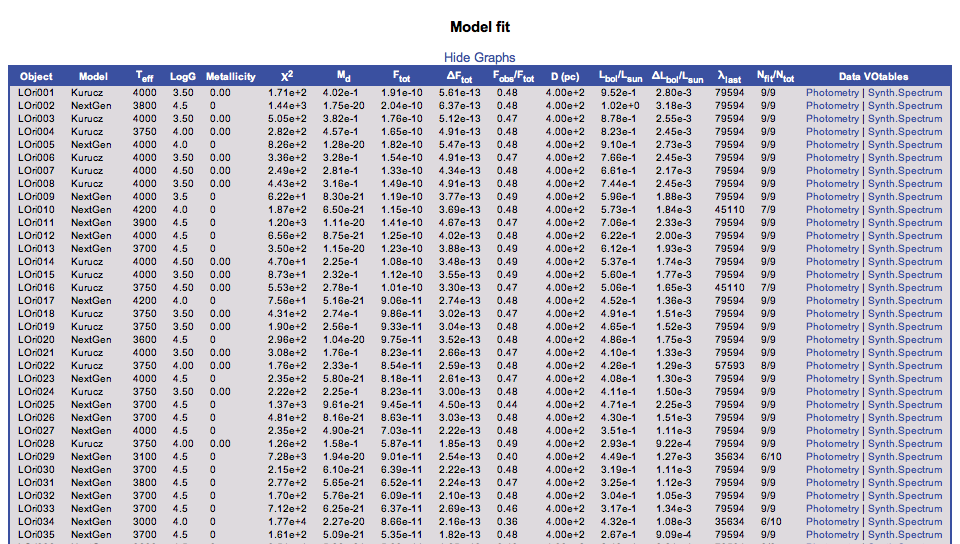
Figure 13: Several rows of the “master-table” with all the fittings.

  1. A summary table (all objects in ASCII or VOTable format) for each entry in the input catalogue with the following fields: identifier, theoretical model collection, effective temperature, surface gravity, reduced-$\chi^{2}$ and multiplicative dilution factor (factor to scale the theoretical data to the observed one; in the case of the models form the Lyon group is related to the ratio between the radius and the distance to the source) of the best fitting, number of data points considered for the calculation of the $\chi^{2}$, the effective wavelength corresponding to the filter of the reddest data-point considered in the fitting process (a flag indicating whether the source has an infrared excess or not), estimated total observed flux, the bolometric luminosity and the ratio of total estimated flux by the total observed flux (a measurement of the bolometric correction applied). Links to the observational photometry as well as to the synthetic photometry and spectra are also provided in this table (see Fig. 13 from Appendix B).

  2. An overall figure with the best fits for all the entries in the input catalog (see Fig. 14 from Appendix B)

• Determination of ages and masses.

  This task was performed by combining the capabilities of the theoretical isochrones and evolutionary tracks service created by the SVO (available at: http://laeff.inta.es/svo/theory/draw/getiso.php?inises=guest) and VOSA. The process is the following:

  1. Access the HR diagram menu, and select the option to create a new diagram.

  2. Decide what collection/s of isochrones and evolutionary tracks (and what ranges of ages and masses) should be used in the interpolation process (in our case we queried the whole range of possibilities, see Fig. 17 from Appendix B). Nowadays the available collections are the following: NextGen isochrones and evolutionary tracks from Baraffe et al. (1998), DUSTY isochrones and evolutionary tracks from Chabrier et al. (2000) and COND isochrones and evolutionary tracks from Baraffe et al. (2003)

     We must note that to perform the interpolation for each particular source, VOSA will use the curves (both isochrones and evolutionary tracks) corresponding to the collection of models for which the best fit, -or the one flagged by the user as best-, was achieved. Otherwise the consistency of the method cannot be guaranteed.

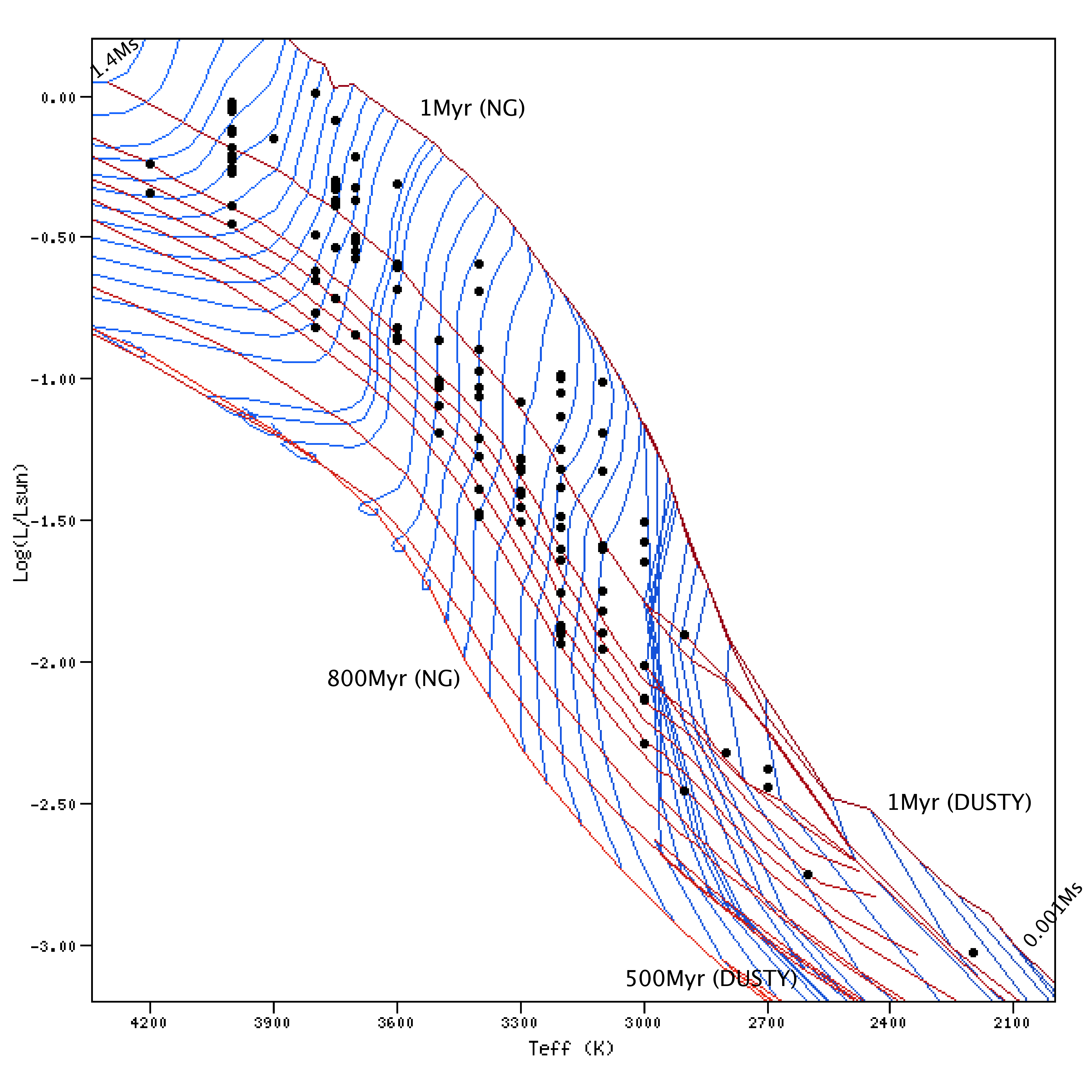
Figure 18: HR diagram of the members of Collinder 69 for which no infrared excess was detected. Isochrones corresponding to ages of 1, 5, 10, 12.5, 16, 20, 25, 50, 100 and 800 Myrs are displayed for the NextGen collection, and those corresponding to ages of 1, 5, 10, 50, 100,120 and 500 Myr for the DUSTY collection. Evolutionary tracks are also displayed for masses between 0.001M☉ and 1.4M☉ (including both, NextGen and DUSTY collections).

  3. Check the estimations given by VOSA (different flags explain possible sources of problems in the estimation process; see the Help menu for further details), and “play” with the sets of isochrones and evolutionary tracks, that should be displayed in order to clarify the HR diagram produced by the application (see as an example Fig 18 from Appendix B, where most of the sources are displayed in an HR diagram, and different sets of isochrones and evolutionary tracks are overplotted).

Once all these estimations are available, we are able to study the cluster as a whole by the statistics derived for the sample of sources, and also study each object individually. The results derived from this study are presented in the next section.

5 Collinder 69 as an example: results

5.1 General outputs

Following the previously described method we have been able to build Spectral Energy Distributions and estimate effective temperatures, gravities and bolometric luminosities for 167 candidate members of Collinder 69, and even infer ages and masses for 145 of these sources in an automatic manner.

Examples of the estimations made through synthetic photometry fittings are shown in Figs. 13, 14, 15 and 16 and the results achieved for each source are shown in Table LABEL:all_param.

Regarding the comparison with theoretical isochrones and evolutionary tracks in the Hertzsprung-Russell diagram, VOSA does not provide estimations of either age or mass for 20 sources ($\sim$12% from the total) due to the peculiar location of these sources in that diagram (see VOSA Help menu for further details on the cases where the interpolation process cannot be completed and no estimation of age and/or mass can be provided).

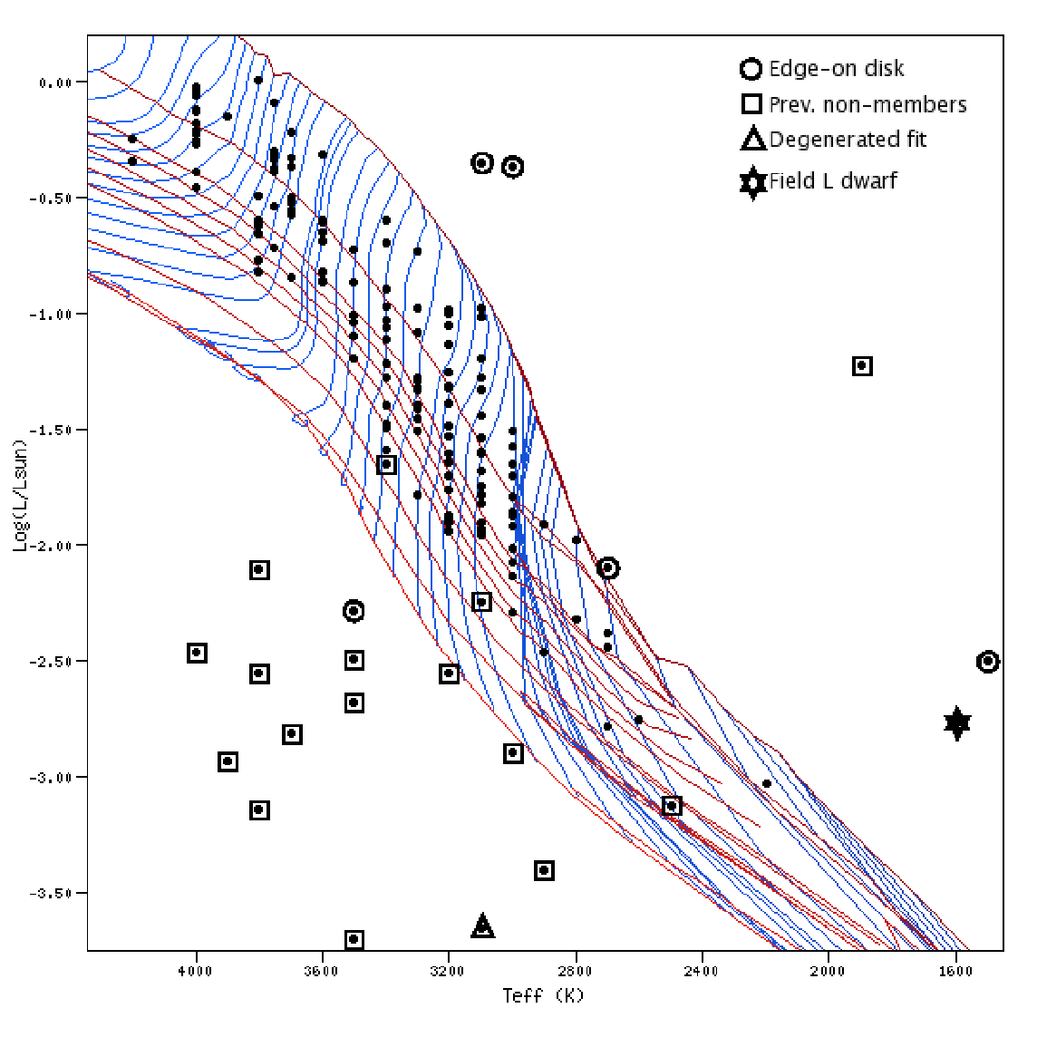
Figure 6: Location in a HR diagram of the “peculiar sources” analyzed in Section 5.3. Squares surround non-members candidates from Barrado y Navascués et al. (2007b); circles are displayed around sources showing infrared excess, and a triangle and a star highlight LOri169 and LOri162, respectively. See text for details.

Besides the case of two special sources, there are two main causes for this peculiar location in the HR diagram: either the source might harbour a close to edge-on disk that reprocess the light emitted from the photosphere of the source (and therefore both, the effective temperature and the bolometric luminosity are underestimated) or the source does not belong to cluster. See Fig. 6 for details on the specific location of the peculiar sources and Subsection 5.3 for the discussion on each particular case.

5.2 Comparison with other methodologies.

In order to test the results provided by VOSA, we have estimated some of the parameters and properties discussed in this work with those derived using other methodologies (mainly based on colours and classical bolometric corrections).

5.2.1 Infrared excesses.

Barrado y Navascués et al. (2007b) studied in detail the Spitzer/IRAC data of the candidates, and based on the criteria developed by Allen et al. (2004) and Hartmann et al. (2005) derived a fraction of members with disks of 25% and 40% for the stellar and substellar population of C69, respectively.

VOSA detects infrared excesses by calculating iteratively the $\alpha$ parameter from Lada et al. (2006). This method provides us with excess fractions of: 32% for candidates with stellar masses (from 0.72 M$\odot$ to 1.15 M$\odot$ ), and 44% for sources with estimated masses $\leq 0.72$ M$\odot$. The differences can be explained by the presence of optically thin disks that mimic the location of single photospheres in the Spitzer/IRAC colour-colour diagrams and are therefore classified as Class III sources.

5.2.2 Effective temperature estimation.

We have derived the effective temperature of our candidates using two different colours ([R-I] and [I-Ks]) and temperature-colour relationships (Bessell 1991 and Leggett 1992). In Fig. 2 we have plotted the relationships mentioned before and overplotted as solid and open circles (diskless and disk harbouring sources) the results obtained with VOSA.
There is a good agreement among the different relationships (specially with the one proposed by Bessell 1991) with offsets of -150K and +100K for the two colours, [R-I] and [I-Ks], respectively. These offsets have already been reported in the literature when comparing temperatures obtained with models and those obtained with colours and temperature scales (see for example Barrado y Navascués et al. 2004a, Barrado y Navascués 2006 and Mohanty et al. 2007).
We have selected one specific case, namely LOri055, where the differences between the temperatures derived from the colors and the one estimated by VOSA are much higher than the mentioned offset. For this case we have forced VOSA to find the best multiplicative factor to fit the SED of this object with NextGen models at temperatures in the range between the lowest (3200K from the [I-Ks] color and the Leggett 1992 temperature scale) and the highest (3600K from VOSA) derived for the source.
In Fig 3 we show the fits obtained when forcing the different temperatures. An inspection of the behaviour of the $\chi^{2}$ of the fits concludes that the temperature proposed by VOSA improves one and a half orders of magnitude the goodness of the fit obtained with the lowest temperature (the one derived with the [I-Ks] colour).

Figure 2: Deredened colors CFHT [R-I] and CFHT–2MASS [I-K] vs. T_eff (obtained with VOSA) for the candidate members of C69. The dotted line represents the relationship derived by Bessell (1991) and the dashed line the one derived by Leggett (1992). Open circles highlight sources harbouring disks.

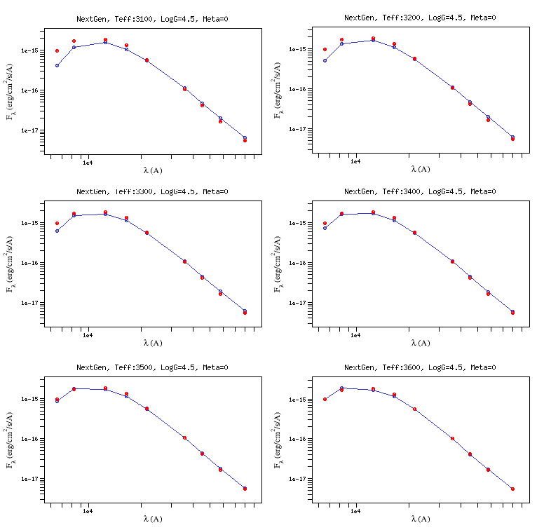
Figure 3: Forced fits to the SED of LOri055 for the range of effective temperatures estimated according to the different methods. According to our calculations, the $\chi^{2}$ improves one and a half orders of magnitude when comparing the 3100K and the 3600K fits.

5.2.3 Bolometric luminosity estimation.

In the case of the computation of the bolometric luminosity, we have applied different bolometric corrections to several photometric bands (I band by Kenyon & Hartmann 1995, J band by Lawson et al. 1996 and Ks band by Tinney et al. 1993) and as can be seen in Fig. 4, there are no systematic differences among the various methods. We must note however, than in our case we use the whole observed SED (but for the wavelength range where some excess is detected) to infer the total emitted flux, and therefore, the better the accuracy of the observations, the better the estimation.

Figure 4: Comparison between the bolometric luminosities estimated with different bolometric corrections applied to various photometrical bands and those obtained with VOSA. Open circles highlight sources harbouring disks.

5.3 Individual sources in C69

As mentioned previously, the location in a T_eff vs L_bol diagram of 20 of our sources made it impossible for VOSA to estimate their ages and masses. Besides, the age estimated with our methodology for three other sources was much higher than the average age estimated in the literature for Collinder 69. We have divided these 23 “peculiar sources” in four groups according to the cause that might explain their location in the HR diagram (we have used the same number code as in Table LABEL:all_param).

1. Sources with infrared excess caused by the presence of a disk. The dust belonging to the disk, reprocesses the light emitted by the central object, and in the cases where the angle of the disk and/or the amount of flaring is high enough, the light from the star can be blocked (see examples of very low mass stars and brown dwarfs surrounded by edge-on disks and the effects on the light from the central object in Fernández & Comerón 2001; Barrado y Navascués et al. 2004a; Pontoppidan et al. 2005; Luhman et al. 2007, and Huelamo et al. 2008, submitted).

   Whenever this is the case, our methodology will underestimate both, the effective temperature and the bolometric luminosity of the central object. We propose this hypothesis as the cause for the peculiar location in the HR diagram of LOri029, LOri034, LOri146, LOri147 and LOri156.

   We must note that we do not see this effect on any of the remaining 24 sources that show infrared excess. See as an example, in Fig 5, the comparison between the best fit obtained for one of the sources classified as “peculiar”, LOri034, and the one achieved for LOri062; in the latter case, all the derived parameters, mainly the age, are consistent with the hypothesis that the source belongs to C69. Thus we consider that a 18% of sources harbouring disks with inclinations or disk structures that block part of the stellar light is a reasonable percentage.

2. Sources previously flagged as possible non-members. Barrado y Navascués et al. (2007b) studied the photometrical properties of the sample, and flagged 16 sources as probable non-members according to these properties. With our methodology, we independently confirm this classification for all 16 sources (see Table LABEL:all_param for the corresponding IDs); 13 of the cases were very clear, since the location of those sources in the HR diagram fell outside the parameter space confined by the isochrones and evolutionary tracks, in the other three cases (LOri101, LOri141 and LOri165), the derived ages (32, 37 and 85 Myr, respectively) were inconsistent with the upper-limit age derived for the whole cluster (12.3–16 Myr, see Subsection 5.4 for details).

3. Degeneracy of the fitting process. In the case of LOri169 no conclusion can be assessed, since the number of points conforming the SED is as low as five (one of them, the R-band magnitude having a very large error), whilst we try to fit four independent parameters.

4. New non-member candidate. Even thought the best fit achieved for LOri162 seems to reproduce quite well the observational data (see Fig 7), the estimated luminosity is not compatible at all with the hypothesis that this object belongs to C69. Its luminosity is much higher than the one expected for a cluster member with the derived effective temperature of 1600 K. This luminosity would imply a radius of the star of $\sim$0.5 R_☉ (assuming a distance of 400 pc and the relationship: $M_{\rm d}=(R/D)^{2}$), whilst according to the isochrones from Baraffe et al. (2003), assuming an age of $\sim$10 Myr, the radius of this object should be $\sim$0.15 R_☉.

   The effective temperature of LOri162 suggests that it might be a field L dwarf that, due to its very low temperature, mimics the colours of the less massive members of Collinder 69. Using the $M_{\rm d}$ factor and assuming a typical radius for 1-5 Gyr dwarfs with the given temperature of 1600 K (according to isochrones from Baraffe et al. 2003), we estimate a distance to this object between 61 and 69 parsecs and a spectral type of L6-L7 according to the T_eff scale by Basri et al. (2000).

Figure 5: Comparison of the best fits achieved for two sources showing infrared excess (open circles for the observed photometry and open triangles joint with dashed line for the synthetic set). On the left hand side, LOri034, a source whose estimated location in the HR diagram does not allow VOSA to infer neither its mass or its age. On the right hand side, LOri062, another source harbouring a disk but for which al the parameters can be estimated by VOSA and with an inferred age of 12.3 Myr, consistent with the range of ages estimated previously, in the literature, for C69.

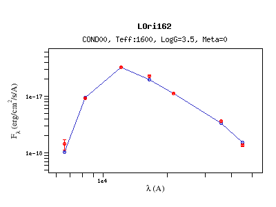
Figure 7: Best fit achieved for LOri162, a possible L field dwarf. We must note that (as mentioned previously in Section 3.2) the SED fitting process is quite insensitive to the surface gravity of the source; besides, at the beginning of the process, we constrained the values of $\log g$ to be between 3.5 and 4.5. Thus, the value of $\log g$ 3.5 shown in the caption should not be taken into account, instead, as reference, the radius assumed when estimating the distance to this source (61-69 parsecs) corresponds to a $\log g$ range of 5.2-5.5

5.4 The cluster C69 as a whole.

Dolan & Mathieu (1999) studied the $\lambda$ Orionis Star Forming Region (which includes the central cluster Collinder 69 and several younger, dark clouds), and, based on the presence of the Li I $\lambda$6708 absorption (in mid-resolution optical spectra) and different theoretical isochrone sets, they concluded that the star formation in this region (high- and low-mass) began 5–7 Myr ago with a dramatic change in the low-mass star formation happening 1–2 Myr ago: either an abrupt cease (through removal of the gas supply), or a burst (caused by star births via cloud compression).

Later on, Dolan & Mathieu (2001) derived a turnoff age of 6–7 Myr based on Strömgren photometry for the massive stars of the cluster.

Finally, Barrado y Navascués et al. (2007b) studied in detail Collinder 69, the older central cluster, and proposed an upper-limit for the age of 20 Myr based on colour-magnitude (optical/near-infrared) diagrams and isochrones by Baraffe et al. (1998), with an optimal age of 5 Myr for the isochrones (Baraffe et al. 2002) corresponding to the DUSTY models.

The methodology presented in this work, provides us with an estimation of the age of the association through the analysis of the statistics of the ages inferred for each individual member of the cluster. We have selected a subsample of 120 sources (out of the total of 167 candidates) that conforms the “least-possible biased” set in the sense that we do not include either sources flagged as possible non-member or sources with infrared excesses whose age estimation might be affected by the effect of the disk on the apparent luminosity of the central object. This set of sources can be considered as a representative sample of the Class III population of Collinder 69 in the 0.014–1.15M_⊙ range of masses. From the 120 sources, the SEDs of three of them are best reproduced with models from the DUSTY collection, while for the remaining 117 the best fitting model always corresponds to either the NextGen or the Kurucz collection. Since different sets of isochrones and evolutionary tracks have to be applied when using the DUSTY models or the NextGen and Kurucz models, we will split our sample in two sets:

• For the three sources where the DUSTY models reproduce the best the observed SEDs, we derive an upper-limit age of 5 Myr

• Among the remaining 117 sources, we find that while 90% of them are younger than 16 Myr, the 3rd Quartile is located at 12.3 Myr; therefore we infer an upper-limit age for Collinder 69 of 12.3-16 Myr.

This final upper-limit of 12.3-16 Myr is consistent with the estimated ages for the cluster by other authors.

A limitation of our methodology is that, since we are performing fitting with four free parameters, a minimum number of six data-points in the observed SED is desirable (to avoid degeneracy). Another issue to take into account is that our results (mainly the derivation of the effective temperatures) are quite discrete, since the minimum step in temperature in the grid of models is 100K.

On the other hand, a great advantage is that the process followed is completely automatic; therefore, if a new (denser) grid of models is published, new observational data become available or new candidate members are detected, our determination of the age can be easily and quickly re-computed.

6 Conclusions

We have presented a new VO-tool, VOSA, developed by the Spanish Virtual Observatory team for this particular scientific case (but with a wider applicability range) to easy the process of calculating synthetic photometry and performing $\chi^{2}$ tests to large sets of fittings as well as to interpolate among collections of isochrones and evolutionary tracks.

When applied to the case of Collinder 69, we have been able to perform the following studies:

1. We have estimated different physical parameters (effective temperatures, gravity, bolometric luminosity, and in most of the cases, mass and age) for 167 candidate members.

2. We have independently confirmed the classification from Barrado y Navascués et al. (2007b) of non-members for 16 of the sources of the sample, and we have added a new possible non-member to this list (LOri162).

3. We have derived an upper-limit for the age of 12.3-16 Myr consistent with previous estimations in the literature.

We must note that VOSA is a very efficient tool; as an example, it only takes $\sim$ 20 minutes to reproduce the whole workflow presented in this paper.

Appendix A: Synthetic photometry.

• Starting point: observed magnitudes (in filters $G_{i}$) that are translated with the zero point $ZP$ into Jy . Thus, we have a flux density per unit of frequency, that is $F_{\nu,G_{i}}$. We can also use $ZP$ for $F_{\lambda}$ and then have another flux density (in this case $F_{\lambda,G_{i}}$).

• The models are functions $F(\lambda)$ with values in $\rm{erg/cm^{2}/s/\AA}$, the filters are functions $G_{1}(\lambda)$ without physical units, but when we normalize the response curves:
  

  $N_{1}(\lambda)=G_{1}(\lambda)/\int_{\lambda}G_{1}(\lambda^{\prime})d\lambda^{\prime}$,
  

  this new function $N_{1}(\lambda)$ is not dimensionless anymore, it has physical units of $\lambda^{-1}$. This is the function that we multiply by the model to obtain a synthetic flux density. So,
  

  $F_{\rm{syn,N}}=\int_{\lambda}F_{\rm{mod},\lambda}(\lambda)\times N_{1}(\lambda)d\lambda$,
  

  with units of $\rm{erg/cm^{2}/s/\AA}$.

• Our observational data-point corresponds to a weighted average of the flux observed through a filter. The process is:

  • The light ($F_{*}$) passes through the filter (a function with values between 0 and 1): $F_{*}\times G_{1}(\lambda)$

  • This “total amount of light” is translated into a density by dividing by the area enclosed by the filter: $\int_{\lambda}G_{1}(\lambda)d\lambda$

• To recover the total flux that was observed through the filter $G_{1}$, we multiply the “observed flux density” by the integral of the flux:
  

  $F_{\rm{total,G_{1}}}=F_{G_{1}}\times\int_{\lambda}G_{1}(\lambda)d\lambda$.
  

  This $F_{\rm{total,G_{1}}}$ has the required physical units of a flux: $\rm{erg/cm^{2}/s}$.

• If we want to compute the bolometric correction using the model, we integrate it:
  

  $F_{M}=\int_{\lambda}F(\lambda)d\lambda$,
  

  subtract the density fluxes corresponding to each filter multiplied by the areas of the filters:
  

  $F_{M}-\sum_{i}(F_{syn,N_{i}}\times\int_{\lambda}G_{i}(\lambda)d\lambda)$),
  

  and add the $F_{\rm{total,G_{i}}}$ calculated in the previous step.
  

  This takes into the account the model to correct from possible intersections among the filters wavelength coverage.

Appendix B: Workflow.

Figure 8: Example of the three lines per object to include in the script. With the first line, the user access the VOSED form; with the second one, a query is performed (to the services available in the VOSED form) around the position written in the fields ra and de within the radius rad (in degrees). Finally with the third line the available data for those coordinates is retrieved. All the information in saved in one “zip-file”.

Figure 9: Part of the input data in the web interface of the SVO SED fitting tool.

Figure 10: Photometrical catalogs to be queried with the respective search radii.

Figure 11: 2MASS photometry found. We will use these JHKs measurements in those objects for which we do not have our own photometrical data.

Figure 12: Range of parameters queried for each collection of synthetic spectra.

Figure 14: First page from the graphical results output.

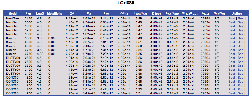
Figure 15: Example of the “small table” showing the 15 best fittings for an individual object (LOri086).

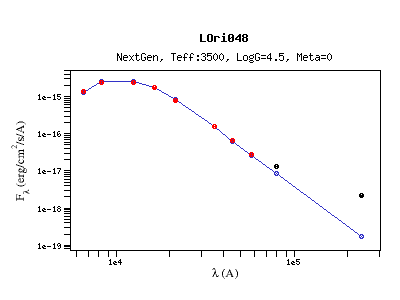
Figure 16: Graphical output from VOSA for a source with infrared excess (LOri048). The black dots highlight those data points not considered when performing the fitting process.

Figure 17: Range of parameters queried for each collection of isochrones and evolutionary tracks.

Table 2: Parameters derived for each individual source of the sample. For some of the sources, we have not been able to interpolate between the isochrones and evolutionary tracks (to infer ages and masses), because of their peculiar location in the HR diagram; we have grouped these sources in four possible categories according to the probable cause for this peculiar location (last column of the table): [1] Source with disk, [2] Previous “non-member” candidates according to the photometric properties (see Barrado y Navascués et al. 2007b for further details), [3] Degenerated fit due the small number of points to be fitted vs number of free parameters, and [4] possible foreground cool source (see Section  5.3 for details on each individual case). [*] For a more detailed analysis in LOri167 see Barrado y Navascués et al. (2007a)

ID	Model	Teff	logg	Fobs/FTot	L(L⊙)	$\Delta$L(L⊙)	Age(Myr)	M(M⊙)	Note
LOri001	Kurucz	4000	3.5	0.48	9.52e-1	2.80e-3	3.0	1.1265	-
LOri002	NextGen	3800	4.5	0.48	1.02e+0	3.18e-3	1.6	0.9508	-
LOri003	Kurucz	4000	3.5	0.47	8.78e-1	2.55e-3	3.2	1.105	-
LOri004	Kurucz	3750	4.0	0.48	8.23e-1	2.45e-3	1.7	0.8613	-
LOri005	NextGen	4000	4.0	0.48	9.10e-1	2.73e-3	3.2	1.113	-
LOri006	Kurucz	4000	3.5	0.47	7.66e-1	2.45e-3	4.0	1.0983	-
LOri007	Kurucz	4000	4.5	0.48	6.61e-1	2.17e-3	5.0	1.0471	-
LOri008	Kurucz	4000	3.5	0.48	7.44e-1	2.45e-3	4.0	1.0962	-
LOri009	NextGen	4000	3.5	0.49	5.96e-1	1.88e-3	5.8	1.0505	-
LOri010	NextGen	4200	4.0	0.48	5.73e-1	1.84e-3	10.0	1.1466	-
LOri011	NextGen	3900	4.5	0.47	7.06e-1	2.33e-3	3.7	1.037	-
LOri012	NextGen	4000	4.5	0.48	6.22e-1	2.00e-3	5.2	1.0544	-
LOri013	NextGen	3700	4.5	0.49	6.12e-1	1.93e-3	2.3	0.7737	-
LOri014	Kurucz	4000	4.5	0.49	5.37e-1	1.74e-3	6.4	1.0473	-
LOri015	Kurucz	4000	3.5	0.49	5.60e-1	1.77e-3	6.3	1.0495	-
LOri016	Kurucz	3750	4.5	0.47	5.06e-1	1.65e-3	3.4	0.8185	-
LOri017	NextGen	4200	4.0	0.48	4.52e-1	1.36e-3	13.7	1.0499	-
LOri018	Kurucz	3750	3.5	0.47	4.91e-1	1.51e-3	3.7	0.8153	-
LOri019	Kurucz	3750	3.5	0.48	4.65e-1	1.52e-3	4.0	0.8102	-
LOri020	NextGen	3600	4.5	0.48	4.86e-1	1.75e-3	2.0	0.624	-
LOri021	Kurucz	4000	3.5	0.47	4.10e-1	1.33e-3	9.9	0.9998	-
LOri022	Kurucz	3750	4.0	0.48	4.26e-1	1.29e-3	4.5	0.8043	-
LOri023	NextGen	4000	4.5	0.47	4.08e-1	1.30e-3	10.0	0.9996	-
LOri024	Kurucz	3750	3.5	0.48	4.11e-1	1.50e-3	4.9	0.8024	-
LOri025	NextGen	3700	4.5	0.44	4.71e-1	2.25e-3	3.2	0.7504	-
LOri026	NextGen	3700	4.5	0.48	4.30e-1	1.51e-3	3.7	0.75	-
LOri027	NextGen	4000	4.5	0.48	3.51e-1	1.11e-3	12.5	0.9586	-
LOri028	Kurucz	3750	4.0	0.49	2.93e-1	9.22e-4	7.4	0.7584	-
LOri029	NextGen	3100	4.5	0.4	4.49e-1	1.27e-3			[1]
LOri030	NextGen	3700	4.5	0.48	3.19e-1	1.11e-3	5.3	0.7237	-
LOri031	NextGen	3800	4.5	0.47	3.25e-1	1.12e-3	7.7	0.8366	-
LOri032	NextGen	3700	4.5	0.48	3.04e-1	1.05e-3	5.9	0.7128	-
LOri033	NextGen	3700	4.5	0.46	3.17e-1	1.34e-3	5.3	0.7231	-
LOri034	NextGen	3000	4.0	0.36	4.32e-1	1.08e-3			[1]
LOri035	NextGen	3700	4.5	0.48	2.67e-1	9.09e-4	6.6	0.7005	-
LOri036	NextGen	3600	4.5	0.49	2.49e-1	8.21e-4	5.0	0.5883	-
LOri037	NextGen	3700	4.5	0.48	2.82e-1	9.78e-4	6.3	0.7033	-
LOri038	NextGen	3800	4.5	0.4	2.55e-1	7.92e-4	10.1	0.8002	-
LOri039	NextGen	3800	4.5	0.47	2.41e-1	8.26e-4	11.1	0.7997	-
LOri040	NextGen	3600	4.5	0.48	2.56e-1	8.55e-4	5.0	0.5922	-
LOri041	NextGen	3400	4.5	0.49	2.54e-1	8.89e-4	2.0	0.3932	-
LOri042	NextGen	3800	4.5	0.47	2.22e-1	7.69e-4	12.6	0.7929	-
LOri043	NextGen	3600	4.5	0.49	2.25e-1	7.95e-4	5.6	0.5744	-
LOri044	Kurucz	3750	3.5	0.48	1.94e-1	6.37e-4	12.6	0.7261	-
LOri045	NextGen	3600	4.5	0.49	2.07e-1	7.30e-4	6.3	0.5703	-
LOri046	NextGen	3800	4.5	0.47	1.71e-1	5.72e-4	18.0	0.7508	-
LOri047	NextGen	3400	4.5	0.47	2.03e-1	7.80e-4	2.5	0.3614	-
LOri048	NextGen	3500	4.5	0.47	1.90e-1	7.20e-4	4.3	0.4516	-
LOri049	NextGen	3800	4.5	0.47	1.52e-1	5.52e-4	20.4	0.7471	-
LOri050	NextGen	3300	4.5	0.44	1.86e-1	6.76e-4	1.9	0.2996	-
LOri051	NextGen	3700	4.5	0.48	1.44e-1	4.64e-4	15.8	0.6508	-
LOri052	NextGen	3600	4.5	0.48	1.52e-1	5.03e-4	9.5	0.5604	-
LOri053	NextGen	3600	4.5	0.48	1.40e-1	5.42e-4	10.0	0.5588	-
LOri054	NextGen	3500	4.5	0.48	1.38e-1	4.66e-4	6.5	0.45	-
LOri055	NextGen	3600	4.5	0.49	1.36e-1	5.28e-4	10.4	0.5584	-
LOri056	NextGen	3400	4.5	0.47	1.27e-1	4.93e-4	4.6	0.35	-
LOri057	NextGen	3400	4.5	0.46	1.07e-1	3.76e-4	5.9	0.35	-
LOri058	NextGen	3500	4.5	0.49	9.87e-2	3.55e-4	10.5	0.4498	-
LOri059	NextGen	3500	4.5	0.48	9.79e-2	3.84e-4	10.7	0.4498	-
LOri060	NextGen	3500	4.5	0.49	9.28e-2	4.03e-4	12.2	0.4498	-
LOri061	NextGen	3300	4.5	0.44	1.06e-1	3.54e-4	3.7	0.2753	-
LOri062	NextGen	3500	4.5	0.46	9.20e-2	3.54e-4	12.3	0.4498	-
LOri063	NextGen	3100	4.0	0.39	1.05e-1	3.37e-4	1.5	0.157	-
LOri064	NextGen	3500	4.5	0.48	8.10e-2	3.05e-4	14.9	0.4496	-
LOri065	NextGen	3400	4.5	0.49	7.76e-2	3.10e-4	9.6	0.3503	-
LOri066	NextGen	3200	4.5	0.5	8.87e-2	3.66e-4	2.9	0.2098	-
LOri067	NextGen	3500	4.5	0.49	6.44e-2	2.94e-4	19.9	0.4469	-
LOri068	NextGen	3400	4.5	0.47	9.32e-2	3.52e-4	7.1	0.3501	-
LOri069	NextGen	3200	4.5	0.5	1.04e-1	4.29e-4	2.4	0.2151	-
LOri070	NextGen	3400	4.5	0.49	6.13e-2	2.78e-4	12.7	0.35	-
LOri071	NextGen	3200	4.5	0.48	7.37e-2	2.98e-4	3.4	0.2028	-
LOri072	NextGen	3100	4.5	0.43	9.69e-2	3.61e-4	1.6	0.1614	-
LOri073	NextGen	3400	4.5	0.46	8.71e-2	3.15e-4	7.9	0.3502	-
LOri074	NextGen	3300	4.5	0.49	8.33e-2	3.18e-4	4.9	0.2619	-
LOri075	NextGen	3200	4.5	0.46	1.01e-1	3.72e-4	2.5	0.2144	-
LOri076	NextGen	3400	4.5	0.48	5.31e-2	2.13e-4	15.8	0.3485	-
LOri077	NextGen	3200	4.5	0.5	5.65e-2	2.57e-4	4.3	0.1965	-
LOri078	NextGen	3300	4.5	0.48	5.28e-2	3.26e-4	8.1	0.2502	-
LOri079	NextGen	3300	4.5	0.5	4.84e-2	2.43e-4	9.5	0.25	-
LOri080	NextGen	3100	4.0	0.49	6.45e-2	2.56e-4	2.5	0.1519	-
LOri081	NextGen	3200	4.5	0.42	4.91e-2	1.96e-4	5.0	0.1783	-
LOri082	NextGen	3300	4.5	0.5	4.77e-2	2.34e-4	9.7	0.25	-
LOri083	NextGen	3300	4.5	0.49	4.69e-2	2.41e-4	9.8	0.25	-
LOri084	NextGen	3300	4.5	0.51	5.18e-2	2.36e-4	8.3	0.2501	-
LOri085	NextGen	3100	4.5	0.43	5.32e-2	2.12e-4	3.1	0.1497	-
LOri086	NextGen	3400	4.5	0.49	4.06e-2	2.04e-4	20.1	0.315	-
LOri087	NextGen	3300	4.5	0.5	4.76e-2	2.49e-4	9.7	0.25	-
LOri088	NextGen	3200	4.5	0.51	4.80e-2	2.64e-4	5.0	0.1762	-
LOri089	NextGen	3300	4.5	0.5	4.04e-2	2.15e-4	11.7	0.2482	-
LOri090	NextGen	3300	4.5	0.46	3.89e-2	1.83e-4	12.4	0.2471	-
LOri091	NextGen	3100	4.0	0.49	4.72e-2	2.32e-4	3.2	0.1432	-
LOri092	NextGen	3300	4.5	0.47	3.94e-2	1.92e-4	12.2	0.2475	-
LOri093	NextGen	3300	4.5	0.49	3.91e-2	2.24e-4	12.3	0.2473	-
LOri094	NextGen	3200	4.0	0.48	4.14e-2	2.10e-4	5.8	0.1743	-
LOri095	NextGen	3300	4.5	0.5	3.53e-2	1.95e-4	12.8	0.243	-
LOri096	NextGen	3100	4.5	0.44	3.66e-2	1.89e-4	4.0	0.1295	-
LOri098	NextGen	3400	4.0	0.49	3.37e-2	2.09e-4	25.0	0.3	-
LOri099	NextGen	3400	4.0	0.47	3.25e-2	1.64e-4	25.1	0.2998	-
LOri100	NextGen	3300	4.5	0.46	3.10e-2	1.80e-4	15.7	0.2337	-
LOri101	NextGen	3400	4.5	0.45	2.60e-2	1.49e-4	31.7	0.2989	-
LOri102	NextGen	3200	4.0	0.48	3.27e-2	2.34e-4	7.6	0.1653	-
LOri103	NextGen	3200	4.5	0.49	2.99e-2	1.50e-4	8.0	0.162	-
LOri104	NextGen	3000	4.0	0.45	3.10e-2	1.54e-4	3.1	0.0899	-
LOri105	NextGen	3200	4.0	0.49	2.51e-2	1.82e-4	10.0	0.1565	-
LOri106	NextGen	3100	4.0	0.45	2.91e-2	1.92e-4	4.9	0.116	-
LOri107	NextGen	3000	3.5	0.49	3.14e-2	2.08e-4	3.1	0.0899	-
LOri108	NextGen	3100	4.5	0.5	2.56e-2	1.75e-4	5.1	0.1103	-
LOri109	NextGen	3200	4.5	0.52	2.28e-2	5.08e-5	11.2	0.1544	-
LOri110	NextGen	3400	4.0	0.48	2.25e-2	1.74e-4	39.8	0.2947	-
LOri111	NextGen	3000	4.0	0.5	2.66e-2	1.86e-4	3.4	0.0882	-
LOri112	NextGen	3100	4.0	0.48	2.49e-2	1.77e-4	5.2	0.1101	-
LOri113	NextGen	3200	4.5	0.49	1.99e-2	4.14e-5	12.7	0.1513	-
LOri114	NextGen	3000	4.0	0.48	2.27e-2	1.73e-4	4.0	0.0822	-
LOri115	NextGen	3300	4.5	0.48	1.64e-2	1.48e-4	31.4	0.2	-
LOri116	NextGen	3200	4.0	0.47	1.75e-2	1.46e-4	15.6	0.1501	-
LOri117	NextGen	3100	3.5	0.5	2.10e-2	4.51e-5	6.3	0.1096	-
LOri118	NextGen	3000	4.0	0.43	1.99e-2	1.36e-4	4.3	0.08	-
LOri119	NextGen	3100	4.0	0.54	1.79e-2	5.97e-5	7.8	0.1084	-
LOri120	NextGen	3100	4.0	0.46	1.65e-2	1.38e-4	8.1	0.1072	-
LOri121	NextGen	3200	4.5	0.48	1.34e-2	1.35e-4	20.0	0.1476	-
LOri122	NextGen	3100	4.0	0.46	1.52e-2	1.37e-4	9.5	0.1057	-
LOri124	NextGen	3200	4.0	0.45	1.30e-2	1.36e-4	20.4	0.1464	-
LOri125	NextGen	3200	4.0	0.46	1.26e-2	1.40e-4	21.3	0.1452	-
LOri126	NextGen	3000	4.5	0.5	1.35e-2	2.80e-5	6.2	0.0736	-
LOri127	DUSTY00	1900	4.5	0.74	6.04e-2	4.21e-4			[2]
LOri128	NextGen	3100	4.0	0.49	1.26e-2	1.67e-4	11.9	0.1022	-
LOri129	NextGen	3000	3.5	0.44	1.61e-2	1.48e-4	5.0	0.075	-
LOri130	NextGen	3200	4.0	0.47	1.16e-2	1.23e-4	24.9	0.1439	-
LOri131	NextGen	3000	3.5	0.5	1.39e-2	1.44e-4	6.1	0.0742	-
LOri132	NextGen	3000	3.5	0.49	1.21e-2	1.53e-4	6.6	0.0723	-
LOri133	NextGen	3800	3.5	0.43	7.85e-3	1.24e-4			[2]
LOri134	NextGen	3100	3.5	0.49	1.17e-2	1.32e-4	12.6	0.1017	-
LOri135	NextGen	3100	3.5	0.46	1.11e-2	1.38e-4	12.9	0.1015	-
LOri136	NextGen	2900	3.5	0.5	1.24e-2	1.80e-4	5.0	0.0602	-
LOri137	NextGen	4000	4.0	0.31	3.50e-3	3.94e-5			[2]
LOri138	NextGen	3000	4.0	0.49	9.78e-3	1.28e-4	8.8	0.0738	-
LOri139	NextGen	3000	4.0	0.49	8.50e-3	1.84e-5	10.1	0.0745	-
LOri140	NextGen	2800	3.5	0.43	1.06e-2	1.23e-4	4.0	0.0405	-
LOri141	NextGen	3100	4.0	0.5	5.69e-3	1.67e-5	36.8	0.1088	-
LOri142	NextGen	3000	4.0	0.51	7.33e-3	1.92e-5	12.6	0.0749	-
LOri143	NextGen	3000	4.0	0.53	7.43e-3	2.29e-5	12.6	0.0749	-
LOri144	NextGen	3800	4.5	0.54	2.85e-3	4.29e-5			[2]
LOri146	NextGen	2700	3.5	0.44	8.00e-3	1.32e-4			[1]
LOri147	NextGen	3500	3.5	0.51	5.24e-3	2.00e-5			[1]
LOri148	NextGen	3000	4.5	0.54	5.19e-3	1.63e-5	20.4	0.0756	-
LOri149	Kurucz	3500	3.5	0.24	2.12e-3	4.22e-6			[2]
LOri150	NextGen	2800	3.5	0.48	4.79e-3	1.31e-4	9.8	0.0472	-
LOri151	NextGen	3200	4.5	0.51	2.81e-3	1.48e-5			[2]
LOri152	NextGen	3500	3.5	0.5	3.26e-3	1.17e-4			[2]
LOri153	NextGen	2900	4.5	0.52	3.49e-3	1.38e-5	25.1	0.0659	-
LOri154	NextGen	2700	3.5	0.48	4.17e-3	1.20e-4	7.9	0.0315	-
LOri155	NextGen	2700	4.5	0.53	3.63e-3	1.11e-5	9.4	0.0336	-
LOri156	COND00	1500	3.5	0.54	3.20e-3	1.43e-5			[1]
LOri157	NextGen	3700	3.5	0.47	1.54e-3	9.04e-6			[2]
LOri158	NextGen	3900	3.5	0.45	1.18e-3	8.72e-6			[2]
LOri159	NextGen	3000	4.5	0.49	1.28e-3	1.17e-5			[2]
LOri160	NextGen	2700	3.5	0.5	1.65e-3	1.02e-5	31.6	0.0467	-
LOri161	NextGen	2600	4.5	0.52	1.77e-3	1.37e-5	16.0	0.0308	-
LOri162	COND00	1600	3.5	0.6	1.71e-3	2.37e-5			[4]
LOri163	DUSTY00	2000	4.0	0.55	1.65e-3	2.13e-5	1.0	0.006	-
LOri164	NextGen	3800	3.5	0.45	7.29e-4	5.92e-6			[2]
LOri165	DUSTY00	2500	3.5	0.51	7.50e-4	1.50e-5	85.3	0.048	[2]
LOri166	DUSTY00	2200	4.5	0.43	9.35e-4	6.94e-6	4.7	0.0136	-
LOri167	DUSTY00	2000	3.5	0.51	1.35e-3	1.85e-5	1.0	0.006	[*]
LOri168	NextGen	2900	4.0	0.45	3.99e-4	7.44e-6			[2]
LOri169	NextGen	3100	4.5	0.45	2.21e-4	6.63e-6			[3]
LOri170	NextGen	3500	3.5	0.45	1.99e-4	8.21e-6			[2]

Table 2: continued.