Measurement of diffusion coefficients of francium and rubidium in yttrium based on laser spectroscopy

Abstract

We report the first measurement of the diffusion coefficients of francium and rubidium ions implanted in a yttrium foil. We developed a methodology, based on laser spectroscopy, which can be applied to radioactive and stable species, and allows us to directly take record of the diffusion time.
Francium isotopes are produced via fusion-evaporation nuclear reaction of a 100 MeV ¹⁸O beam on a Au target at the Tandem XTU accelerator facility in Legnaro, Italy. Francium is ionized at the gold-vacuum interface and Fr⁺ ions are then transported with a 3 keV electrostatic beamline to a cell for neutralization and capture in a magneto-optical trap (MOT). A Rb⁺ beam is also available, which follows the same path as Fr⁺ ions. The accelerated ions are focused and implanted in a 25 $\mu$m thick yttrium foil for neutralization: after diffusion to the surface, they are released as neutrals, since the Y work function is lower than the alkali ionization energies. The time evolution of the MOT and the vapor fluorescence signals are used to determine diffusion times of Fr and Rb in Y as a function of temperature.

I Introduction

In many experiments with radioactive atoms, elements are produced as ions and then neutralized. The most important requirement for a neutralization system is the fast release of neutral atoms, with respect to their radioactive decay time. In particular, in our francium experiment at INFN’s National Laboratories in Legnaro, Italy Atutov et al. (2003), we produce Fr ions that have to be neutralized before accumulation in a magneto-optical trap. The system must be very efficient, as a large sample of Fr atoms is requested for nuclear decay, atomic parity violation and permanent electric dipole studies.

Our apparatus follows the scheme of the Stony Brook experiment Gomez et al. (2006), where many measurements on Fr have been performed so far. Francium isotopes are produced at the Tandem accelerator facility in Legnaro via the fusion-evaporation reaction

$${}^{197}\mbox{Au}+^{18}\mbox{O}\longrightarrow^{215-x}\mbox{Fr}+x\mbox{n}.$$

With an energy of the primary beam around 100 MeV, we are able to produce Fr isotopes in the mass number range 208-211. These isotopes have a lifetime that is long enough for laser cooling and trapping. The system is at the moment optimized for maximum production of ²¹⁰Fr, which has a half-life of 191 s. Francium atoms are ionized at the surface of the gold target and transported through an electrostatic beamline at an energy of 3 keV towards a spectroscopic cell designed for laser cooling. The ionic beam is focused on a 99.96% pure yttrium foil, placed inside the cell on the opposite side with respect to the entrance aperture. In order to be able to detect the trap, we have to optimize all the processes, from production to laser trapping. With only a few days of beamtime per year, it is not convenient to test the setup with francium: we decided to use stable rubidium, always available in high quantities. To this purpose a Rb dispenser was placed in the reaction chamber near the target: Rb atoms that arrive on the gold surface are ionized and injected in the electrostatic line, following the same path as Fr. A sketch of the apparatus is shown in Fig. 1.

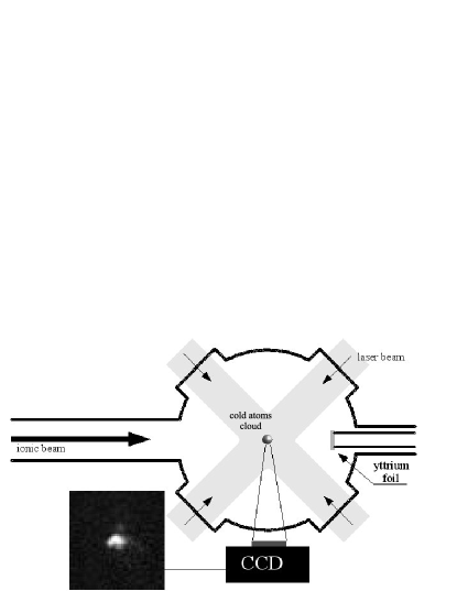
Figure 1: Scheme of the experimental setup (the two anti-Helmholtz coils for magneto optical trapping are not shown). In the inset, an image of the cold Fr trap is reported. The image is not to scale.

Yttrium has a work function $\phi=3.1$ eV, that is lower than Fr and Rb ionization potentials, respectively $\mathcal{I}_{\mbox{Fr}}=4.08$ eV and $\mathcal{I}_{\mbox{Rb}}=4.18$ eV. The probability of release in neutral form at the Y surface is close to unity, according to the Saha-Langmuir equation

$$\frac{n_{+}}{n_{a}}=\frac{g_{+}}{g_{a}}\exp{\left(\frac{\phi-\mathcal{I}}{k_{B}T}\right)}~{},$$

where $n_{+}$ and $n_{a}$ are the number of desorbed ions and neutral atoms, $g_{+}$ and $g_{a}$ are the statistical weights due to degeneracy of the ion and atom ground states respectively ($\frac{g_{+}}{g_{a}}=\frac{1}{2}$ for alkalis), and $k_{B}$ is Boltzmann’s constant. This ratio is $\sim 6\times 10^{-6}$ at 1000 K.

In spite of the fact that high temperature enhances diffusion, we fixed an upper limit of 1050 K in order to preserve the cell coating Stephens et al. (1994) and hence not to compromise the trapping efficiency. This is a limitation because melting point of Y is $T_{m}$=1799 K, and because the total release fraction grows with the ratio $T/T_{m}$ Melconian et al. (2005). In this context, our goal was to check whether the efficiency of the neutralizer was high enough at a chosen temperature. So far the release efficiency of radioactive atoms embedded in the neutralizer has been measured by monitoring their nuclear decay Melconian et al. (2005). We used atomic laser spectroscopy to observe the time evolution of the released neutrals and deduce the diffusion time. We also took advantage of the extraordinary sensitivity given by our magneto-optical trap, which allows us to observe as few as 50 atoms.

II 1-D Diffusion model

If an ion is implanted at a given depth inside the Y foil, then it has to diffuse towards the surface to be released in atomic form. In order to achieve a good release efficiency, the time necessary to complete this process has to be small compared with the radioactive lifetime of the investigated atom. Since the transverse dimension of the ionic beam is much larger than the penetration depth, we can use the one-dimensional diffusion equation for the concentration $N(x,t)$ of the diffusing species in the Y foil at the distance $x$ from the surface:

$$\frac{\partial N(x,t)}{\partial t}=D\frac{\partial^{2}N(x,t)}{{\partial x}^{2}}-\Gamma_{r}N(x,t)+\varphi(x,t).$$

$\Gamma_{r}$ is the radioactive decay rate ($\Gamma_{r}=0$ for Rb), $D$ the diffusion coefficient and $\varphi(x,t)$ is the incoming current of ions impinging on the Y foil. Note that $\varphi(x,t)$ is not directly observable: it has to be deduced from the measurement of its integral $I(t)$ (the total current) on the neutralizer volume and from the presumed implantation distribution, discussed in Sections II.1 and II.2.

Empirically, we expect that the dependence of $D$ on the temperature follows the Arrhenius’ law

$$D=D_{\infty}\exp{\left(-\frac{E_{a}}{k_{B}T}\right)}.$$

$E_{a}$ is the activation energy and $D_{\infty}$ is the theoretical asymptotic value of $D$ for large temperatures. The characteristic diffusion time is given by

$$\tau_{d}=\frac{d^{2}}{4D}~{},$$

where $d$ is the mean implantation depth of ions in the Y foil.

II.1 Pulsed regime

In the case of $N_{0}$ ions all implanted at the same distance $d$ from the surface at the time $t=0$, i.e. $N(x,0)=N_{0}\delta(x-d,0)$, the diffusion equation with $\varphi(x,t)\equiv 0$ has an analytical solution: the flux of neutral atoms released in the cell at the time $t$ is given by Liatard et al. (1997)

$$F_{0}(t)=\frac{2N_{0}}{\sqrt{\pi}}\sqrt{\frac{\tau_{d}}{t^{3}}}\exp{\left(-\frac{\tau_{d}}{t}\right)}\exp{(-\Gamma_{r}t)}.$$ (1)

For an implantation distribution with a finite extent, the function can be different, specially for $t<\tau_{d}$; in a rough approximation, this difference can be taken into account with a correction factor, which is expected to be of the order of unity in the case that $\Gamma_{r}\ll\tau_{d}^{-1}$ Liatard et al. (1997). For instance, Melconian et al. take the case of a distribution modelled by a Gaussian times a linear term, with a characteristic implantation depth $d$ Melconian et al. (2005). In this case, the function becomes

$$\tilde{F}_{0}(t)=\frac{N_{0}}{2}~{}\frac{1}{\tau_{d}}~{}\frac{1}{(1+t/\tau_{d})^{3/2}}~{}\exp(-\Gamma_{r}t).$$ (2)

II.2 Continuous regime

If a constant total ionic current $I_{0}$ is sent to the neutralizer starting at the time $t=0$, for stable isotopes ($\Gamma_{r}=0$) we see that the neutralized released current takes the form

$$F(t)=\int_{0}^{t}I_{0}\;\frac{F_{0}(t-t^{\prime})}{N_{0}}\;dt^{\prime}=I_{0}\left[1-\mbox{erf}\left(\sqrt{\frac{\tau_{d}}{t}}\right)\right].$$ (3)

In the case of the implantation distribution considered by Melconian et al., we have

$$\tilde{F}(t)=I_{0}\left[1-\frac{1}{\sqrt{1+t/\tau_{d}}}\right].$$ (4)

We will see in the following that we can operate in two modes. If we let ions accumulate in cold yttrium for a certain time and then we turn on the neutralizer (pulsed mode), all the implanted ions are released according to Eqs. (1) or (2). Instead, if we turn on the ionic beam with the neutralizer already working (continuous mode), we are in the case described by Eqs. (3) or (4).

In our model of the release process, we neglect the contribution of desorption to the release time. We can reasonably assume that, due also to the accuracy of such a model, discussed in Section IV.2, desorption contribution is well included in our uncertainty. In any case, as also discussed in Ref. Melconian et al. (2005), the diffusion coefficients derived from our data analysis can be properly considered as upper limits.

III Magneto-optical trapping dynamics

After being released, atoms can be either directly detected in the vapor phase (rubidium), or they can be first collected in a small volume (about 1 mm³) in order to enhance our sensitivity (rubidium and francium). The confinement is provided by a magneto-optical trap in the standard configuration: six trapping and repumping laser beams respectively tuned on the D2 and D1 lines, and a constant gradient magnetic field provided by two anti-Helmholtz coils.

The total number of atoms in the cell, when the six laser beams and the magnetic field are present, is the sum of two components: the number of trapped atoms $N_{t}$ and the number of atoms in the vapor phase $N_{v}$ which is supposed to be at thermal equilibrium with the cell walls. The time evolution of $N_{t}$ and $N_{v}$ is well described by the coupled rate equations de Mauro (2007)

$$\left\{\begin{aligned} \dot{N_{t}}&=LN_{v}-CN_{t}-\Gamma_{r}N_{t}\\ \dot{N_{v}}&=-(L+W)N_{v}+CN_{t}-\Gamma_{r}N_{v}+f~{},\end{aligned}\right.$$ (5)

where $L$ is the rate related to the loading process (the product $LN_{v}$ represents the number of atoms per unit time loaded from the vapor to the MOT), $C$ is the rate describing the collisional loss of atoms from the MOT ($CN_{t}$ represents the number of trapped atoms per unit time which go back from trap to vapor phase due to collisions with background gas in the cell) and $W$ is the rate characterizing the loss of atoms from the vapor phase ($WN_{v}$ represents the number of atoms per unit time definitively lost to the vacuum system or by chemisorption to the cell walls). $f$ is the current of atoms released by the neutralizer and suitable for trapping. We did not report the quadratic terms due to collisions between trapped atoms, which are negligible. We can find the quasi-stationary state solution $\dot{N_{t}}\simeq\dot{N_{v}}\simeq 0$ of Eqs.(5) under the condition $\dot{f}/f\ll C,W$ (slowly varying incoming current hypothesis):

$$\left\{\begin{aligned} N_{t}(t)&=\frac{L}{(W+\Gamma_{r})(C+\Gamma_{r})+L\Gamma_{r}}\;f(t)\\ N_{v}(t)&=\frac{C+\Gamma_{r}}{(W+\Gamma_{r})(C+\Gamma_{r})+L\Gamma_{r}}\;f(t)\end{aligned}\right.$$ (6)

In practice, provided that $f$ varies with a time scale much longer than $1/C$, we obtain that the detected number of trapped atoms and the total number of atoms in the vapor phase are proportional to the released current at any time. Therefore, the measurement of the trap signal or of the fluorescence signal directly gives all the information about diffusion inside the neutralizer. This constitutes an innovative way of measuring the diffusion coefficient, with respect to other experiments that measure the release efficiency by detecting the radioactivity from the residual ions in the neutralizer.

IV Measurements methods

IV.1 Vapor fluorescence and MOT detection

At room temperature the Rb vapor density is high enough to be directly detected through resonant excitation and looking at the atomic fluorescence. In order to minimize changes in the apparatus we made measurements by only switching off the trapping magnetic field, but keeping in place the six laser beams. The laser frequency is scanned across the whole profile of the D2 Rb line to search for the maximum signal. Fluorescence light is in this case collected on a Si photodiode. We tried different spectroscopic schemes and we obtained the best signal-to-noise ratio with the one described above. In the case of francium, it is not possible to directly observe the atomic vapor fluorescence, because the signals are extremely weak. The solution is given by the MOT, that allows to accumulate Fr (and also Rb) atoms in a small volume at low temperature. In fact the signal increases by about two orders of magnitude because of Doppler broadening elimination and, at low densities, far from saturated vapor pressures, by several orders of magnitude because of higher densities. As already stressed, we are able to detect traps of only a few tens of atoms. Atomic fluorescence from trapped atoms is detected by a CCD cooled camera (Fig. 1). A dedicated software performs background subtraction, to reduce the contribution of scattered light to the noise, and real time correction for laser intensity fluctuations de Mauro (2007). The detector was accurately calibrated and the software directly gives the number of atoms in the cold cloud.

IV.2 Continuous and pulsed regime

When we turn on the ionic beam and send it on a hot neutralizer set at a constant temperature, we expect the spectroscopic signals to be well described by Eqs. (3) and (4) (Fig. 2). The main advantage of this method is that the temperature of yttrium is kept constant during the measurement, and the vacuum conditions for the MOT are very stable. We analyzed Rb data taken in the continuous regime for several temperatures. The comparison of the results for the fits with Eq. (3) and with Eq. (4) showed an interesting feature, which allows us to estimate the impact of the implantation distribution on our results: while the two resulting curves are almost indistinguishable, assuming a sharp implantation distribution yields diffusion times that are systematically lower by a factor 0.7 with respect to the results obtained in the hypothesis of an extended initial distribution such as the one used by Melconian et al.. This means that the accuracy for the measured diffusion coefficient is anyway limited at the 30% level by the theoretical model, also for previous experiments Melconian et al. (2005); Liatard et al. (1997).

Figure 2: Fluorescence signal from the Rb atoms desorbed by the neutralizer. The curve from Eq. (4) (with an additional offset) was fitted to the experimental data.

In order to enhance the signals, it is possible to operate in a pulsed mode. We let the ions accumulate in cold yttrium: at room temperature, the diffusion coefficient is very small, and the ions stay embedded in the neutralizer. When the neutralizer is turned on, the atoms are released all together in a time scale of the order of $\tau_{d}$, according to Eq. (1) or (2). In practice, for both Rb and Fr we usually kept the ionic current on for 600 s (which corresponds to more than three ²¹⁰Fr radioactive half-lives). This method gave excellent results to estimate the neutralizer release efficiency, and to determine the best operating temperature for our neutralizer.

V Experimental results

V.1 Rubidium

Most measurements have been done in the pulsed mode, because of the higher signal-to-noise ratio. We obtained a set of data for each neutralizer operating temperature: the main goal was to optimize the yttrium temperature in order to obtain a good release efficiency.

The function $G(G_{0},S_{0},\tau_{d},t_{0};t)=G_{0}+S_{0}/(1+(t-t_{0})/\tau_{d})^{3/2}$, corresponding to the flux $\tilde{F}_{0}(t)$ (Eq. (2)), was fitted to each acquired data set, with the free parameters $G_{0}$, $S_{0}$ and $\tau_{d}$ (Fig. 3). The offset $G_{0}$ is due to the presence of Rb impurities in yttrium: even with fresh neutralizers, never exposed to Rb current, we detect Rb vapor in the cell coming from the heated yttrium foil. Note that $t_{0}$ is not left as a free parameter, because it is totally correlated with the other parameters $S_{0}$ and $\tau_{d}$: for any value $t_{0}^{\prime}$, we can find the parameters $S_{0}^{\prime}=S_{0}/(1+\frac{t_{0}^{\prime}-t_{0}}{\tau_{d}})^{3/2}$ and $\tau_{d}^{\prime}=\tau_{d}~{}(1+\frac{t_{0}^{\prime}-t_{0}}{\tau_{d}})$, such that $G(G_{0},S_{0},\tau_{d},t_{0};t)\equiv G(G_{0},S_{0}^{\prime},\tau_{d}^{\prime},t_{0}^{\prime};t)$. Therefore, $t_{0}$ is manually set to the time at which the signal begins rising, just after turning on the neutralizer. Since the neutralizer does not reach the operating temperature instantaneously, $t_{0}$ is affected by an error corresponding to the signal rising time.

The initial part of the curve critically depends on the way the neutralizer is turned on, and on the initial distribution of ions inside yttrium (cf. Eqs. (1) and (2)). Therefore, we decided to consider data after a time $t_{\text{in}}$, corresponding to a signal which is equal to 3/4 of the maximum signal for the whole curve (Fig. 3).

Figure 3: Fluorescence signal from Rb neutralized ions in the pulsed mode and fit curve from Eq.(2), at a temperature of 960 K.

Figure 4: Diffusion time of Rb in yttrium as a function of temperature, fitted with the Arrhenius’ function (Eq.(7)).

Release time data are consistent with Arrhenius’ law for the diffusion coefficient $D$. Our experimental results are then fitted accordingly (Fig. 4):

$$\tau_{d}=\tau_{1000}\;\exp{\left[\frac{E_{a}}{k_{B}}\left(\frac{1}{T}-\frac{1}{1000\mbox{K}}\right)\right]}$$ (7)

where $\tau_{1000}$ is the diffusion time at 1000 K; fit parameters are both the time $\tau_{1000}$ and the activation energy $E_{a}$. The choice of such a fit function lies in the fact that $\tau_{1000}$ better describes the diffusion time in the temperature range of our measurements, while $\tau_{\infty}$ would be affected by a larger error, due to the extrapolation to infinite temperature. Results of fit are $\tau_{1000}=(6.1\pm 2.3)$ s and $E_{a}=(1.8\pm 0.4)$ eV. We used the TRIM code Ziegler (2007) to evaluate the mean implantation depth for Rb in Y at 3 keV, which gives a value of 4.9 nm. From this data we can then deduce the diffusion coefficient at 1000 K:

$$D_{1000}=\frac{d^{2}}{4\tau_{1000}}=(1.0\pm 0.4)\times 10^{-14}\;\mbox{cm}^{2}\mbox{s}^{-1}.$$

We also performed measurements on Rb using the MOT detection method, to prepare the Fr measurements and to test our diffusion model also for the MOT signal evlution. Experimental data and fit curve for Rb MOT in pulsed regime are shown in Fig. (5). A good agreement was found between data and model, and also with the results obtained from vapor fluorescence detection described above. The fit procedure used in this case is discussed in Section V.2.

Figure 5: Rubidium MOT in pulsed regime: experimental data and fit curve. Neutralizer temperature was about 960 K

V.2 Francium

The diffusion time of francium in yttrium has been measured using the magneto-optical trap. We operate in the pulsed mode in order to get higher signals: we use the same method as for Rb, with detection of trapped atoms. With a collisional rate $C$ of about 0.5 s^-1, we checked that the condition $\dot{f}/f\ll C,W$ is verified for all the acquired data.

As compared to vapor fluorescence data, MOT fluorescence is quite difficult to analyze in the pulsed mode, to deduce the diffusion time. When we turn on the neutralizer, francium atoms come out of yttrium along with many other impurities already contained in the neutralizer (as Rb): vacuum suddenly deteriorates, and then slowly comes back to the equilibrium value. Since the coefficient $C$ in Eq. (6) strongly depends on vacuum quality, in the first part of the curve ($t-t_{0}<\tau_{d}$) $C$ depends on time and it is not easy to interpret the data. However, retaining only data with $t-t_{0}\gg\tau_{d}$ cannot be a solution, because in this regime $S_{0}$ and $\tau_{d}$ are totally correlated (it is not possible to distinguish them in the fitting procedure). Our compromise was to consider data after a time $t_{\text{in}}$ that corresponds to a signal which is equal to half the maximum signal of the whole curve (Fig. 6). For these data vacuum effects are satisfactorily reduced and the order of magnitude is reasonable.

It was not always easy to reach convergence in fits: in practice, we kept $S_{0}$ and $\tau_{d}$ as free parameters, and we set the offset and $t_{0}$ to a reasonable value for each fit. In some cases, $\tau_{d}$ and $S_{0}$ were too correlated to obtain a good convergence: we had to repeat the fitting procedure with $S_{0}$ set by hand to realistic values. The error for the obtained parameters includes several contributions: statistical error from the fit and uncertainties of $G_{0}$ and $t_{0}$.

We saw in Section V.1 that the methodology was checked with Rb atoms. The agreement between MOT and vapor data demonstrates the validity of our measurements and of the fitting procedure.

We expect to be able to improve our results. Because the presented measurements were initially intended to test the final release efficiency, in terms of number of atoms $N_{0}$ rather than release time $\tau_{d}$, we preferred to begin with the pulsed method, which gives higher signals and higher signal-to-noise ratios. Nevertheless, in our limited beam-time we managed to acquire data in the continuous regime for one neutralizer temperature: we remind that in this regime we expect no vacuum-related problems. The analysis for the obtained curve gave very promising results, in agreement with the pulsed method.

Figure 6: Trapped Fr fluorescence and fit curve according to Eq. (2) with $\Gamma_{r}=3.633\times 10^{-3}\;\mbox{s}^{-1}$. The exposure time of the CCD camera was set to 1 s.

Figure 7: Diffusion time of Fr in Y as a function of temperature: experimental data and fit curve according to Arrhenius’ law.

In Fig. 7 the results for the fitted parameter $\tau_{d}$ are reported as a function of temperature. We performed release time measurements using also the $\alpha$ decay rate signal, and we obtained similar results, at least as order of magnitude, thus confirming the consistency of our method. Fit results according to Eq.(7) are:

$$\tau_{1000}=(4.1\pm 2.5)\;\mbox{s}\qquad E_{a}=(1.8\pm 1.1)\;\mbox{eV}$$

An activation energy of $E_{a}=(1.59\pm 0.15)$ eV was measured for ³⁷K in yttrium in Ref. Melconian et al. (2005), so our results for both Fr and Rb are consistent with literature. We used the TRIM code Ziegler (2007) to evaluate the mean implantation depth for Fr in Y at 3 keV, which gives a value of 5.1 nm. The measured diffusion coefficient at 1000 K is then

$$D_{1000}=(1.6\pm 0.9)\times 10^{-14}\;\mbox{cm}^{2}\mbox{s}^{-1}$$

This is to our knowledge the first determination of diffusion time of francium ions in yttrium and the first time that diffusion parameters are derived from the study of the time evolution of the signal from a magneto-optical trap.

According to Ref. Liatard et al. (1997) it is possible to define a parameter $\varepsilon(\Gamma_{r})=\exp{(-2\sqrt{\Gamma_{r}\;\tau_{d}})}$, which takes into account the loss of atoms due to nuclear decay during the diffusion towards surface. This is the so-called “release fraction” which gives the percentage of radioactive ions neutralized before the decay and then suitable for trapping. In other words, one could interpret $\varepsilon(\Gamma_{r})$ as a sort of neutralization efficiency. From the diffusion time measurement we determine the release fraction as a function of temperature as shown in Fig. 8.

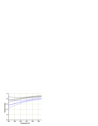
Figure 8: (Color online) Calculated release fraction vs temperature for isotope 210 (black curve) and 209 (blue curve), according to Arrhenius’ law and $E_{a}$ and $\tau_{1000}$ given from our fit. Dashed curves give the uncertainty interval.

Note that our measurements of the diffusion coefficients for ²¹⁰Fr allow us to predict the release fraction for ²⁰⁹Fr, which we also produce and trap, since we can reasonably suppose that diffusion features are identical for the two isotopes with negligible mass difference. Because the apparatus was not optimized for the production of this isotope, we did not perform systematic measurements on ²⁰⁹Fr. Nevertheless, our prediction of $\varepsilon$ provides an estimation of the optimal conditions for the ²⁰⁹Fr neutralization: due to shorter lifetime of about 72 s, we expect ²⁰⁹Fr neutralization to be more efficient at higher temperatures with respect to ²¹⁰Fr (Fig. 8). Analog considerations can be applied to ²¹¹Fr: due to very similar radioactive lifetime, the curve calculated for ²¹¹Fr is indistinguishable from the ²¹⁰Fr one.

VI Conclusions

We measured for the first time the diffusion parameters of francium and rubidium ions in yttrium. The methodology that we developed takes advantage of laser spectroscopy techniques, and of the very high sensitivity offered by laser cooling and trapping. Since we directly measure diffusion times, our method can be considered complementary of release efficiency measurements by nuclear decay. Another advantage is the possibility to measure diffusion coefficients also for stable elements.
Experimental data are consistent with the diffusive model considered, demonstrating the validity and the potential useful application of our method. The diffusion coefficient is determined together with an activation energy consistent with previous measurements. For Fr, a release fraction of more than 80% is obtained for the 210 isotope at 1050 K, while for the short-lived 209 isotope we predict a release fraction around 70% at the same temperature.

References

- Atutov et al. (2003) S. N. Atutov, R. Calabrese, V. Guidi, B. Mai, E. Scansani, G. Stancari, L. Tomassetti, L. Corradi, A. Dainelli, V. Biancalana, et al., J. Opt. Soc. Am. B 20 (2003).
- Gomez et al. (2006) E. Gomez, L. A. Orozco, and G. D. Sprouse, Rep. Prog. Phys. 69, 79 (2006).
- Stephens et al. (1994) M. Stephens, R. Rhodes, and C. Wieman, J. Appl. Phys. 76, 3479 (1994).
- Melconian et al. (2005) D. Melconian, M. Trinczek, A. Gorelov, W. P. Alford, J. A. Behr, J. M. D’Auria, M. Dombsky, U. Giesen, K. P. Jackson, T. B. Swanson, et al., Nucl. Instrum. Methods A 538, 93 (2005).
- Liatard et al. (1997) E. Liatard, G. Gimond, G. Perrin, and F. Schussler, Nucl. Instrum. Methods A 385, 398 (1997).
- de Mauro (2007) C. de Mauro, Ph.D. thesis, Università degli Studi di Siena (2007).
- Ziegler (2007) J. Ziegler, http://www.srim.org (2007).