Delayed currents and interaction effects in mesoscopic capacitors

Abstract

We propose an alternative derivation for the dynamic admittance of a gated quantum dot connected by a single-channel lead to an electron reservoir. Our derivation, which reproduces the result of Prêtre, Thomas, and Büttiker for the universal charge-relaxation resistance, shows that at low frequencies, the current leaving the dot lags after the entering one by the Wigner-Smith delay time. We compute the capacitance when interactions are taken into account only on the dot within the Hartree-Fock approximation and study the Coulomb-blockade oscillations as a function of the Fermi energy in the reservoir. In particular we find that those oscillations disappear when the dot is fully ‘open’, thus we reconcile apparently conflicting previous results.

I Introduction

The low-frequency conductance of a mesoscopic conductor with capacitive elements has recently attracted renewed interest due to the experimental verification GL of the fascinating prediction made in Ref.  B00, (see also Refs.  B0, ,  B1, and  ROSA, ), concerning the universal value of the charge-relaxation resistance. The setup of the device is depicted in Fig. 1: a mesoscopic system consisting of a quantum dot coupled by a single-channel wire to an electron reservoir. A macroscopic gate, which is connected to an ac source, is placed nearby. This source induces an ac potential on the dot, $U(\omega)$, and consequently a current, $I(\omega)$, is flowing between the dot and the reservoir, such that $I(\omega)=g(\omega)U(\omega)$, where $g(\omega)$ is the frequency-dependent conductance of the dot. Note that in this formalism the current $I$ is created by the effective potential on the dot (denoted here by $U$) that includes screening effects, and not by the bare potential, $V$. As is shown in Ref.  B1, , the total ac conductance (often referred to as admittance) of this device is $[g^{-1}_{\rm gate}(\omega)+g^{-1}(\omega)+(-i\omega C_{0})^{-1}]^{-1}$, where $C_{0}$ is the capacitance of the dot and the nearby gate, and $g_{\rm gate}(\omega)$ is the conductance between the gate and the wire connecting it to the voltage source. However, for large enough $C_{0}$ and $g_{\rm gate}(\omega)$, the ac conductance of the device, which is the quantity probed in the experiment, is given by $g(\omega)$.

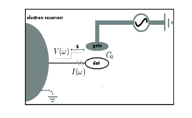
Figure 1: The mesoscopic capacitor: the ac source excites a periodic accumulation of charges on the gate and the latter affects the charges on the dot via the potential $V$ created in-between the dot and the gate. This in turn causes the ac current $I$ flowing between the dot and the electron reservoir.

The ac conductance of noninteracting electrons can be presented in terms of the scattering matrix of the mesoscopic system (see Refs.  B1, ,  BUTTI, , and  YEHOSHUA, ). When the dot is connected by a single-channel lead to an electron reservoir, as in Fig. 1, the ac conductance is

$$g(\omega)=\frac{e^{2}}{h}\int_{E_{F}-\hbar\omega}^{E_{F}}\frac{dE}{\hbar\omega}\Bigl{(}1-S^{\ast}(E)S(E+\hbar\omega)\Bigr{)}\ ,$$ (1)

where the scattering matrix $S(E)$ is just a phase factor

$$S(E)=\exp[i\phi(E)]\ .$$ (2)

In writing down Eq. (1) we have assumed low enough temperatures, such that the Fermi functions factor $f(E)-f(E+\hbar\omega)$ is replaced by unity within the indicated integration limits; $E_{F}$ is the Fermi energy of the reservoir. The universal value of the charge-relaxation resistance predicted in Ref.  B1, and confirmed experimentally GL , emerges upon comparing the low-frequency expansion of Eq. (1) with the ac conductance, $g_{a}(\omega)$, of a conventional capacitor, $C$, connected in series to a dc-resistance, $R$,

$$g_{a}(\omega)=-i\omega C+\omega^{2}C^{2}R+{\cal O}(\omega^{3})\ .$$ (3)

One then finds for $R$ the value $h/2e^{2}$, which is half the quantum unit of the resistance, and in particular is independent of the scattering properties of the quantum dot, embedded in the scattering matrix $S(E)$. The capacitance, on the other hand, is given by $C=(e^{2}/2\pi)\phi^{\prime}(E_{F})$, where $\phi^{\prime}(E_{F})$ is the energy-derivative of the phase (2) at the Fermi energy. Since it is related to coherent properties of the device, this capacitance is usually referred to as the “quantum capacitance” B1 ; GL .

Performing ac measurements without contacts or with only one ohmic contact might be very useful for molecules due to the difficulty in properly and nondestructively contacting them. However, the interest there is in specific, more than in universal, properties. The quantum capacitance of a molecule may well therefore be of genuine interest.

The quantum capacitance is expected to exhibit mesoscopic oscillations, related to Coulomb blockade (CB), as function of the Fermi energy. BS The discussion of this effect necessitates the consideration of electronic correlations in the system, notably on the quantum dot. The original derivation of the low-frequency conductance used a Hartree-type approximation to capture the effects of electronic interactions. B1 This was followed up in Ref.  ROSA, , and studied in great detail in particular in Ref.  BS, . However, the latter reference reports on the persistence of those oscillations even when the dot is fully open to its lead (see Fig. 2 and Sec. V of Ref.  BS, ). This result has been obtained for relatively small values of $E_{c}/{\rm d}$, where $E_{c}$ is the charging energy of the dot and ${\rm d}$ is the mean-level spacing at the Fermi level. Nonetheless, one should note that in the other limit, $E_{c}\gg{\rm d}$, MatveevMT has shown that these oscillations should disappear for a sufficiently large dot which is completely open.

In this paper we expound on the two components of the low-frequency conductance, the charge-relaxation resistance, $R$, and the quantum capacitance, $C$. In the next section we present an alternative derivation of the frequency-dependent conductance (1), which emphasizes the different roles played by the current flowing into the dot and the one leaving it. In particular, our derivation sheds some light on the origin of the intriguing observation of a universal-valued charge-relaxation resistance, describing it in terms of a delayed current. Our simple model does not include dephasing effects. For a clear discussion of those see Ref.  DEPHASING, . In Sec. III we analyze the effects of the Coulomb interaction on the dot. We treat the electronic interactions within a full Hartree-Fock calculation. In particular, we examine in Sec. III the result of Ref.  BS, concerning the persistence of mesoscopic oscillations in the capacitance when the dot is completely open, and show that by including systematically all Fock correlations, the results are reconciled with the prediction of Matveev MT . Namely, we find that in a completely open dot with a large number of equally spaced levels, the on-dot interactions do not induce CB effects in the capacitance. Compared to Matveev MT , our treatment is not confined to strong interactions only. It is, however, limited by our use of the mean-field approach. Moreover, our theory ignores effects related to disorder which may modify the results considerably (see for example Ref.  CHAOTIC, ).

II Delayed currents

Here we show that the total current $I(t)$ (see Fig. 1) can be written in the form

$$I(t)=\frac{e^{2}}{h}\Bigl{(}U(t)-U(t-\tau)\Bigr{)}\ ,$$ (4)

where $\tau$ is the Wigner-Smith SM delay time,

$$\tau=\hbar\frac{\partial\phi(E)}{\partial E}\ ,$$ (5)

evaluated at the Fermi energy COM2 . This result applies to the low-frequency ($\omega<<1/\tau$) components of $U(t)$ or to a slowly varying $U(t)$. The result (4) gives a vivid interpretation of the dynamics of the device. The current flowing between the dot and the reservoir consists of an ingoing (into the dot) component, $I_{\rm in}=(e^{2}/h)U(t)$, which responds instantaneously to the effective voltage $eU(t)$, and an outgoing one (away from the dot), $I_{\rm out}=(e^{2}/h)U(t-\tau)$, which lags after the effective voltage. The incoming current is excited around the region where the potential drop occurs (see Fig. 1) and flows towards the dot; it obeys the Landauer formula for an ideal single-channel wire. After a delay time $\tau$ that current is reflected back and flows towards the reservoir as $I_{\rm out}$, again obeying the Landauer formula for a perfect conductor. This means that in terms of the Wigner-Smith delay time $\tau$, the conductance $g(\omega)$ is

$$g(\omega)=\frac{e^{2}}{h}(1-e^{i\omega\tau})\ .$$ (6)

Comparing the low-frequency expansion of $g(\omega)$ of Eq. (6) with the classical ac conductance of the equivalent RC circuit, Eq. (3), yields for the charge-relaxation resistance, $R$, and the capacitor, $C$, the expressions B1

$$R=\frac{h}{2e^{2}}\ ,\ \ C=\frac{e^{2}}{h}\tau\ .$$ (7)

Note that $\tau=2RC$. The proof of Eq. (4), or alternatively, Eqs. (6) and (7), is based on the linear-response expression for the ac conductance in the framework of the scattering formalism, as derived e.g., in Refs.  B1, ,  BUTTI, , and  YEHOSHUA, . Our derivation (unlike previous treatments employing the scattering formalism) makes use of the spatial dependence of the current operator in order to identify separately the incoming and the reflected current operators. This separation, in turn, allows for the calculation of the respective partial response functions of the two currents. As a result, one finds that the incoming current obeys the Landauer formula for a perfect (single-channel) wire, while the reflected one is delayed by the Wigner-Smith time, leading finally to Eq. (4). This provides a qualitative interpretation of the results of Ref.  B1, .

We employ the results of Ref.  B1, to show that (details are given in Appendix A) the current operator can be written in the form

$$\hat{I}(x,t)=\hat{I}_{\rm in}(x,t)-\hat{I}_{\rm out}(x,t)\ ,$$ (8)

where $\hat{I}_{\rm in}$ denotes the current operator of particles moving into the dot,

$$\hat{I}_{\rm in}(x,t) =\frac{e}{h}\int dEdE^{\prime}e^{i(E-E^{\prime})t/\hbar}$$

$$\times a^{\dagger}(E)a(E^{\prime})e^{i(|k(E^{\prime})|-|k(E)|)x}\ ,$$ (9)

and $\hat{I}_{\rm out}$ is the current operator for particles moving out of the dot into the reservoir,

$$\hat{I}_{\rm out}(x,t) =\frac{e}{h}\int dEdE^{\prime}e^{i(E-E^{\prime})t/\hbar}S^{\ast}(E)S(E^{\prime})$$

$$\times a^{\dagger}(E)a(E^{\prime})e^{i(|k(E)|-|k(E^{\prime})|)x}\ .$$ (10)

Here $a(E)$ ($a^{\dagger}(E)$) creates (destroys) a carrier of energy $E$ moving into the dot, whose momentum is $k(E)$.

The current operators are used in the Kubo linear-response formula to compute the (measurable, in principle) currents flowing in the system. In the present case, the perturbation (resulting from the ac voltage source to which the macroscopic gate of Fig. 1 is connected) induces periodic charge accumulation on the dot and on part of the lead to which it is connected. We assume that the resulting potential is roughly uniform on the dot and beyond it, until it drops to zero further away in the lead due to screening, say at the point $x=-\delta$ (see Fig. 1; the origin of the $x-$axis is taken at the entrance to the dot). The temporal derivative of the charge accumulation yields the current at $x=-\delta$. Measuring the current at the entrance to the lead then gives the conductance of the dot in the form

$$g(\omega)=\frac{1}{\hbar\omega}\int_{0}^{\infty}dte^{i(\omega+i\eta)t}\langle[\hat{I}(0,t),\hat{I}(-\delta,0)]\rangle\ ,\ \ \eta\rightarrow 0^{+}\ .$$ (11)

The magnitude of $\delta$, within a rather large range of values, does not really matter for the total current. Actually, it is argued in Refs.  B1, and  BUTTI, that for the relevant (relatively low) frequencies $\omega$, the factor $\exp[i(k-k^{\prime})x]$ [see Eqs. (9) and (10)] may be replaced by unity. Indeed, the expression (1) is obtained upon setting $\delta$ of Eq. (11) equal to zero. However, in order to establish the different temporal behaviors of the incoming and the outgoing currents it is useful to retain $\delta\neq 0$ for the time-being.

Evidently, inserting Eq. (8) for the decomposition of the current operator into the Kubo formula (11), the conductance $g(\omega)$ is decomposed as well into

$$g=g_{\rm in,in}+g_{\rm out,out}-g_{\rm in,out}-g_{\rm out,in}\ ,$$ (12)

where $g_{\rm a,b}$ stands for the response of the current flowing in the a$-$direction to the current (due to the perturbation) along the b$-$one. We show in Appendix A that two response functions out of the four listed in Eq. (12) vanish, $g_{\rm out,out}(\omega)=g_{\rm in,out}(\omega)=0$, and hence there is no response to the perturbing outgoing current (since $\delta$ is chosen as positive, see Eqs. (41) and the following discussion). The remaining response functions are finite. We show in Appendix A that $g_{\rm in,in}(\omega)=e^{2}/h$, leading to an instantaneous response of the incoming current to the perturbing incoming current, and consequently to the first term in Eq. (4). On the other hand, $g_{\rm out,in}(\omega)=(e^{2}/h)\exp[i\omega\tau]$ [see Eq. (42)], causing a delayed outgoing current.

III Capacitance oscillations

Monitoring the frequency dependence of the mesoscopic conductance enables one to study the ‘quantum capacitance’, GL ; B1 ; BS in particular its dependence on the transmission of the quantum dot and on the Fermi energy. As mentioned above, for ‘open dots’, previous theoretical studies of the dependence of Coulomb oscillations on the dot-wire coupling appear to be in a certain conflict MT ; BS . In this section we attempt to shed some light on this intriguing issue.

For noninteracting electrons, the capacitance of the quantum dot [see Eq. (7)] is given by the Wigner-Smith time, i.e., by the energy-derivative of the transmission phase at the Fermi level. A possible route to include the effect of interactions on the dot is hence to find the modifications they cause in the scattering matrix, Eq. (2). Such a procedure, adopted in Ref.  BS, , necessitates the reduction of the (interacting) Hamiltonian to a quadratic form, e.g., by using an approximation to treat the interactions (see below). However, once the Hamiltonian is reduced to a quadratic form, one may circumvent the calculation of the scattering matrix by using the Friedel sum-rule HEUSON which relates the scattering-matrix phase to the total occupancy of the dot levels, $N_{d}$. As shown in Ref.  BLY, ,

$$\frac{d\phi(E_{F})}{dE}=2\pi\frac{dN_{d}(E_{f})}{dE}\ ,$$ (13)

and therefore the capacitance is given by the energy-derivative of this total occupancy.

The Hamiltonian of our model system (see Fig. 1) is written as

$${\cal H}={\cal H}_{\rm wire}+{\cal H}_{\rm dot}+{\cal H}_{\rm tun}\ .$$ (14)

We describe the single-channel wire by a one-dimensional tight-binding Hamiltonian,

$${\cal H}_{\rm wire}=-J\sum_{\ell=-\infty}^{-1}\Bigl{(}c^{\dagger}_{\ell}c_{\ell-1}+{\rm hc}\Bigr{)}\ .$$ (15)

Here, $c_{\ell}$ ($c^{\dagger}_{\ell}$) destroys (creates) an electron on the $\ell$th ‘site’ of the wire (the lattice constant of the entire system is taken as unity), and $J$ is the hopping amplitude (in energy units) between adjacent sites. The Hamiltonian of the dot, ${\cal H}_{\rm dot}$, includes the single-particle part and the interactions. COM5 The former is a ‘continuation’ of the single-channel wire, while the interactions are described by the charging Hamiltonian,

$${\cal H}_{\rm dot}=-J\sum_{\ell=1}^{n_{d}-1}\Bigl{(}c^{\dagger}_{\ell}c_{\ell-1}+{\rm hc}\Bigr{)}+\frac{E_{c}}{2}\Bigl{(}\hat{N}-\frac{n_{d}}{2}\Bigr{)}^{2}\ ,$$ (16)

where $E_{c}$ is the charging energy, $\hat{N}$ is the number operator on the dot,

$$\hat{N}=\sum_{\ell=0}^{n_{d}-1}c^{\dagger}_{\ell}c_{\ell}\ ,$$ (17)

and $n_{d}$ denotes the number of sites on the dot. Finally, the tunneling Hamiltonian of Eq. (14) gives the coupling between the dot and the wire,

$${\cal H}_{\rm tun}=-J_{0}\Bigl{(}c^{\dagger}_{0}c_{-1}+c^{\dagger}_{-1}c_{0}\Bigr{)}\ .$$ (18)

The magnitude of the capacitance oscillations is determined by the strength of the coupling between the dot and the wire.

The model Hamiltonian (14) is close in spirit to the system considered by Matveev, MT who has employed advanced techniques to treat the effects of the electronic correlations. Here we confine ourselves to the simpler type of approximations used in the previous studies of the ac conductance BS . However, since one of our aims in this section is to explore the relation between the results of Büttiker and Nigg BS and those of Ref.  MT, , it is useful to show the equivalence of the Hamiltonian (14) and the Hamiltonian used in Ref.  BS, .

To this end, one diagonalizes the single-particle part of the dot Hamiltonian Eq. (16), by introducing the unitary transformation

$$d^{\dagger}_{n}=\sqrt{\frac{n_{d}}{2}}\sum_{\ell=0}^{n_{d}-1}\sin\Bigl{(}\frac{\pi(\ell+1)}{n_{d}+1}\Bigr{)}c^{\dagger}_{\ell}\ ,$$ (19)

which turns the dot Hamiltonian into the form

$${\cal H}_{\rm dot}=\sum_{n=1}^{n_{d}}E_{n}d^{\dagger}_{n}d_{n}+\frac{E_{c}}{2}\Bigl{(}\hat{N}-\frac{n_{d}}{2}\Bigr{)}^{2}\ ,$$ (20)

where the number operator is $\hat{N}=\sum_{n=1}^{n_{d}}d^{\dagger}_{n}d_{n}$ and the energy levels are given by

$$E_{n}=-2J\cos(\pi n/(n_{d}+1))\ .$$ (21)

In addition, the unitary transformation (19) changes the tunneling part of the Hamiltonian into

$${\cal H}_{\rm tun} =\sum_{n=1}^{n_{d}}V_{n}\Bigl{(}c^{\dagger}_{-1}d_{n}+{\rm hc}\Bigr{)}\ ,$$

$$V_{n} =-\sqrt{\frac{2}{n_{d}}}J_{0}\sin\Bigl{(}\frac{\pi n}{n_{d}+1}\Bigr{)}\ ,$$ (22)

such that in the transformed system each level on the dot is coupled to the wire.

The energy levels on the dot, $E_{n}$, are almost equally-spaced around mid-band (zero energy in our scheme) when the dot is rather large, $n_{d}\gg 1$. Equation (21) then can be approximated by

$$E_{n}\simeq n{\rm d}\ ,\ \ {\rm d}=J\frac{2\pi}{n_{d}}\ ,$$ (23)

where ${\rm d}$ denotes the level spacing. In practice, we allow $n$ to be within the range $|n|\leq N$ (i.e., $N\ll n_{d}$ or equivalently $Nd<<J$) thereby truncating the spectrum to $2N+1$ levels. These levels are also approximately uniformly coupled to the wire, with coupling energy

$$V=-J_{0}\sqrt{\frac{{\rm d}}{J\pi}}\ .$$ (24)

In this way, our model Hamiltonian (14) becomes identical to the one employed in Ref.  BS, .

In order to find the capacitance of the dot described by the truncated Hamiltonian, we need to find the quantum average of the occupations of the dot levels. This is accomplished by treating the interactions in the Hartree-Fock approximation, replacing the interaction term of the dot Hamiltonian ${\cal H}_{\rm d}$ by

$${\cal H}_{\rm HF}=E_{c}\sum_{m,n}\Bigl{(}Q_{nn}d^{\dagger}_{m}d_{m}-Q_{nm}d^{\dagger}_{m}d_{n}\Bigr{)}\ ,$$ (25)

where the generalized occupancies, $Q_{nm}$,

$$Q_{nm}=\langle d^{\dagger}_{n}d_{m}\rangle\ ,$$ (26)

are computed self-consistently. Thus, the Hamiltonian of the dot becomes

$${\cal H}_{\rm dot}=\sum_{n}n{\rm d}d^{\dagger}_{n}d_{n}+{\cal H}_{\rm HF}\ .$$ (27)

The occupations of the dot levels are given by the diagonal ($n=m$) generalized occupancies, but their determination requires the computation of the non-diagonal ones as well.

The generalized occupancies can be found from the imaginary part of the dot Green function, in which the coupling to the wire appears as the width of the dot levels

$$Q_{nm}=\int_{-\infty}^{E_{F}}\frac{dE}{\pi}{\rm Im}\Bigl{[}{\cal H}_{\rm dot}-E-i\gamma\Bigr{]}^{-1}_{nm}\ .$$ (28)

The form of the width $\gamma$ is a somewhat subtle point. In our simple model, the dot is entirely open when $J=J_{0}$ [see Eqs. (15) and (18)], and then $\gamma$ becomes of the order of the level spacing, ${\rm d}$. However, it is more realistic to imagine a point contact coupling the dot and the wire, and then the transmission between the dot and the wire depends on the energy of the moving electrons. We hence follow Ref.  BS, and adopt the result of Brouwer and Beenakker BB , which relates the level widths of a very large dot to the transmission coefficient ${\cal T}$ of the point contact,

$$\gamma({\cal T})=\frac{{\rm d}}{\pi{\cal T}}\Bigl{(}1-\sqrt{1-{\cal T}}\Bigr{)}^{2}\ .$$ (29)

The transmission coefficient of a point contact modeled by a saddle point potential varies rather sharply with the Fermi energy of the reservoir. We have chosen the parameters of this potential so that

$${\cal T}(E_{F})=\frac{1}{1+e^{-2E_{F}/{\rm d}}}\ .$$ (30)

Note that the dot is open when $E_{F}$ exceeds vastly the level spacing, and then the width $\gamma$ tends to its maximal value (of the order of the level-spacing). When $-E_{F}$ vastly exceeds ${\rm d}$, the point contact closes, and concomitantly the width $\gamma$ vanishes.

The computations described below have been carried out for a dot with 61 levels ($N=30$) in the truncated Hamiltonian. The Fermi energy $E_{F}$, the charging energy $E_{c}$, and the width $\gamma$ [see Eq. (29)] are measured in units of the level-spacing ${\rm d}$, with $-2\leq(E_{F}/{\rm d})\leq 5$, $\gamma$ changing accordingly following Eq. (30), and $E_{c}$ taking various values, indicated on the figures.

A simple iteration algorithm has been used to solve Eq. (28) for the generalized occupancies. In order to achieve reliable convergence, Eq. (28) has been solved gradually: instead of directly solving with the chosen parameter set (using some arbitrary initial values), we have solved with a series of sets, beginning with a certain trivial one (e.g., for $E_{c}=0$ or for a very weak coupling) and varying the parameters gradually till the desired set is reached. For each set, the iteration algorithm has been initiated with the solution of the previously solved set.

Our computation and the one presented in Ref.  BS, differ in their treatment of the generalized occupancies. Whereas we keep the non-diagonal occupancies, those have been discarded by Büttiker and Nigg.BS These non-diagonal occupancies vanish when the dot is isolated. It is therefore not surprising that our results coincide with those of Ref.  BS, when the dot is weakly coupled to the lead. However, when the coupling is strong and the dot is ‘open’, these non-diagonal occupancies, albeit being rather small (see Fig. 2) play a crucial role.

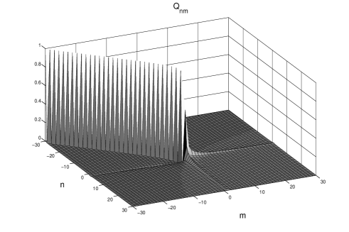
Figure 2: Generalized occupancies, $Q_{nm}$, of an open dot with $E_{c}={\rm d}$. The Fermi energy is chosen such that level number 3 is half full ($\langle d^{\dagger}_{3}d_{3}\rangle=0.5$) and therefore the off-diagonal occupancies are maximal. Still, the largest ones are smaller than $0.15$.

A detailed comparison between our results and those obtained according to the approximation carried out in Ref.  BS, is shown in Figs. 3 and 4. Those figures depict the capacitance as function of the Fermi energy (solid lines). Figure 3 exhibits the capacitance computed without the non-diagonal occupancies, i.e., according to the procedure of Ref.  BS, , while Fig. 4 shows the same quantity computed in the presence of the non-diagonal occupancies, i.e., employing the full Hartree-Fock approximation of the model. In all panels, the dotted lines represent the transmission between the dot and lead. At small values of the Fermi energy, i.e., on the left part of each plot, the dot is loosely coupled to the lead [see Eq. (30)], and the Coulomb-blockade peaks are well-defined, separated from each other by ${\rm d}+E_{c}$. As the transmission increases, i.e., on the right side of each plot, the capacitance oscillations are more smeared. However, the smearing is much more pronounced when all the Hartree-Fock terms are included in the computations: whereas in Fig. 3 the peaks persist and their heights even increase with interaction strength, they decay into a weaker oscillation which does not increase with the interaction strength in Fig. 4.

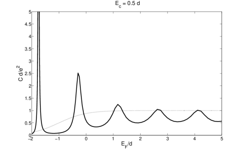
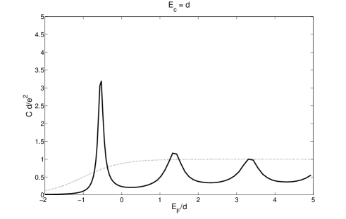
Figure 3: The capacitance as a function of the Fermi energy computed without including the non-diagonal occupancies, for two values of $E_{c}/{\rm d}$ (solid lines). The dashed lines are the transmission at the entrance of the dot computed from Eq. (30). The capacitance is measured in units of $e^{2}/{\rm d}$.

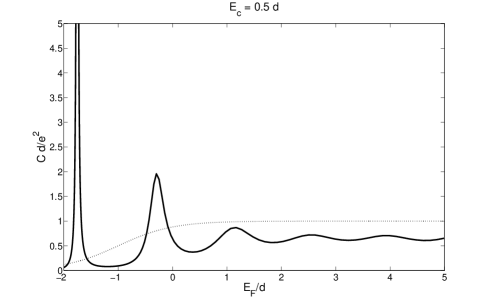
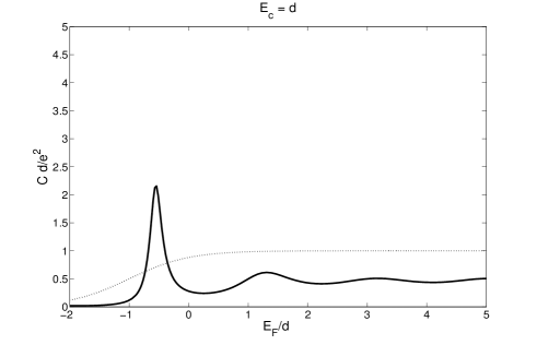
Figure 4: The capacitance as a function of the Fermi energy computed with the non-diagonal occupancies, for two values of $E_{c}/{\rm d}$ (solid lines). The dashed lines are the transmission at the entrance of the dot computed from Eq. (30). The capacitance is measured in units of $e^{2}/{\rm d}$.

The weaker oscillations appearing on the right side of each of the plots in Fig. 4 are not a signature of the CB effect but rather an artifact related to the truncation of the spectrum. Note that these oscillations appear already in the interaction-free case ($E_{c}=0$) [see Fig. 4 ] and decay rather than increase as the interaction strengthens. Figure 5 presents the decay of these oscillations as a function of the dot-level number, $N$. Thus, at least up to order $1/N$, the Hartree-Fock approximation establishes the vanishing of Coulomb blockade effects in an open dot, even for small values of $E_{c}/{\rm d}$.

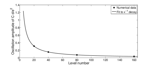
Figure 5: The peak height of the interaction-free capacitance C, measured in units of $e^{2}/{\rm d}$, as function of the level number ($2N+1$).

Using a different approach, Matveev MT predicted the vanishing of CB effects in open quantum dots, for large values of $E_{c}$/d. Figure 6 portrays the capacitance for $E_{c}/{\rm d}=10$ , both for the case where the non-diagonal occupancies are included (solid line) and for the case when they are absent (dashed line). Note the disappearance of the CB peaks in the first case, compared to the second one.

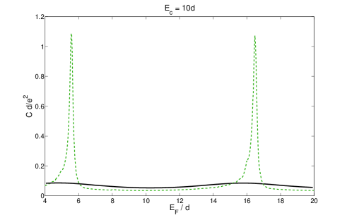
Figure 6: The capacitance as a function of the Fermi energy computed with and without off-diagonal occupancies (solid and dashed lines, respectively), for $E_{c}=10{\rm d}$. The transmission throughout the scanned energy range is essentially one, following Eq. (30). The capacitance is measured in units of $e^{2}/{\rm d}$.

IV Conclusions

We have considered here the ac conductance of a quantum dot connected by an ideal single-channel wire to an electron reservoir and driven by a nearby gate at frequency $\omega$. This conductance can, at low frequencies, be represented in terms of a conventional RC circuit. It was predicted in Ref.  B1, and confirmed experimentally in Ref.  GL, that R is given by half the quantum resistance and that $C$ exhibits, in general, quantum oscillations. These are due to the varying density of states of the dot.

In Sec. II we showed that the results for the ac conductance could be interpreted in terms of an “incoming” current, synchronous with the driving voltage and an “outgoing” current delayed by $\tau$ with respect to the latter, [see Eq. (4)] where $\tau$ is the Wigner-Smith delay time of the dot, given by the derivative of the reflection phase of the dot with respect to the incoming energy. The identification of these two currents is obtained using a space-dependent linear response analysis. Equations (7) follow almost trivially, and provides a vivid physical picture for the results.

In Sec. III we address the issue of Coulomb blockade oscillations in the limit in which the dot is strongly coupled to the lead (dot-level width comparable with its level spacing). Reference  BS, found, from a modified Hartree procedure, that the oscillations persist. On the other hand, it had been found by Matveev MT that they should vanish in the limit of a fully open dot. We have treated the problem including the full Hartree-Fock approximation, i.e., taking into account the non-diagonal occupancies. We have found that the CB oscillations do vanish in the limit of a open dot, up to possible $1/N$-type corrections, where N is the number of the levels on the dot. this result follows from a Hartree-Fock treatment, and does not require the more elaborate treatment of the electronic correlations on the dot MT .

*

Appendix A The current operators in the scattering formalism

In the scattering-formalism approach one expands the current operator, $\hat{I}$, in terms of operators which create (destroy) the incoming or the outgoing electrons COM3 ,

$$\hat{I}(x,t) =\sum_{\sigma\sigma^{\prime}}\int dEdE^{\prime}e^{i(E-E^{\prime})t/\hbar}$$

$$\times a^{\dagger}_{\sigma}(E)a_{\sigma^{\prime}}(E^{\prime})I_{\sigma\sigma^{\prime}}(x;E,E^{\prime})\ .$$ (31)

Here, $a^{\dagger}_{\sigma}(E)$ [$a_{\sigma}(E)$] creates (destroys) a carrier of energy $E$ moving in the direction defined by $\sigma$: $\sigma=+$ denotes incoming (into the dot) particles, whose momentum is positive, while $\sigma=-$ denotes the particles going away from the dot. These operators obey the anti-commutation relations

$$[a^{\dagger}_{\sigma}(E),a_{\sigma^{\prime}}(E^{\prime})]_{+}=\delta_{\sigma\sigma^{\prime}}\delta(E-E^{\prime})\ ,$$ (32)

and are normalized such that

$$\langle a^{\dagger}_{\sigma}(E)a_{\sigma^{\prime}}(E^{\prime})\rangle=\delta_{\sigma\sigma^{\prime}}\delta(E-E^{\prime})f(E)\ ,$$ (33)

where $f(E)$ is the Fermi function of the particles in the reservoir. The two sets of operators, those belonging to the incoming particles and those of the outgoing ones are related by the scattering matrix,

$$a_{-}(E)=S(E)a_{+}(E)\ .$$ (34)

The matrix elements of the quantum-mechanical current density operator in the scattering states which appear in Eq. (31) are

$$I_{\sigma\sigma^{\prime}}(x;E,E^{\prime})=\frac{e}{h}\frac{v_{k}+v_{k^{\prime}}}{2\sqrt{|v_{k}v_{k^{\prime}}|}}e^{i(k^{\prime}-k)x}\ ,$$ (35)

where $v_{k}$ is the velocity of the $k-$ state, $v_{k}=\partial E/(\hbar\partial k)$, and $k=\sigma|k|\equiv k(E)$ (and similarly, $k^{\prime}=\sigma^{\prime}|k^{\prime}|\equiv k(E^{\prime})$).

At low enough frequencies, the relevant energies in Eq. (31) are close to the Fermi level. Then, the magnitude of both $v_{k}$ and $v_{k^{\prime}}$ is $v_{F}$, the Fermi velocity, and they only differ in their signs. COM4 It follows that the velocity factor of Eq. (35) becomes $\sigma\delta_{\sigma\sigma^{\prime}}$, i.e.,

$$I_{\sigma\sigma^{\prime}}(x;E,E^{\prime})=\frac{e}{h}\delta_{\sigma\sigma^{\prime}}\sigma e^{i(k^{\prime}-k)x}\ .$$ (36)

As a result one may unambiguously distinguish in the current operator Eq. (31) the incoming current operator, $\hat{I}_{\rm in}$, for which both $\sigma$ and $\sigma^{\prime}$ are positive, from the outgoing one, $\hat{I}_{\rm out}$, for which $\sigma=\sigma^{\prime}=-$, leading to Eqs. (9) and (10). For brevity, we have omitted in the main text the subscript $+$ from the operators $a$ and $a^{\dagger}$.

We next consider the partial response functions that appear in Eq. (12). Each of those involves the same thermal average [see Eqs. (9), (10), and (11)],

$$\langle [a^{\dagger}(E)a(E^{\prime}),a^{\dagger}(\tilde{E})a(\tilde{E}^{\prime})]\rangle$$

$$= \delta(E-\tilde{E}^{\prime})\delta(E^{\prime}-\tilde{E})(f(E)-f(E^{\prime}))\ ,$$ (37)

where $a(E)\equiv a_{+}(E)$, and $a^{\dagger}(E)\equiv a^{\dagger}_{+}(E)$. Performing also the temporal integration, we find

$$g_{\rm in,in}(\omega) =i\frac{e^{2}}{h^{2}\omega}\int dEdE^{\prime}\frac{f(E)-f(E^{\prime})}{E-E^{\prime}+\omega+i\eta}e^{i(|k(E^{\prime})|-|k(E)|)\delta}\ ,$$

$$g_{\rm out,out}(\omega) =i\frac{e^{2}}{h^{2}\omega}\int dEdE^{\prime}\frac{f(E)-f(E^{\prime})}{E-E^{\prime}+\omega+i\eta}e^{i(|k(E)|-|k(E^{\prime})|)\delta}\ ,$$

$$g_{\rm in,out}(\omega) =i\frac{e^{2}}{h^{2}\omega}\int dEdE^{\prime}\frac{f(E)-f(E^{\prime})}{E-E^{\prime}+\omega+i\eta}e^{i(|k(E)|-|k(E^{\prime})|)\delta}S(E)S^{\ast}(E^{\prime})\ ,$$

$$g_{\rm out,in}(\omega) =i\frac{e^{2}}{h^{2}\omega}\int dEdE^{\prime}\frac{f(E)-f(E^{\prime})}{E-E^{\prime}+\omega+i\eta}e^{i(|k(E^{\prime})|-|k(E)|)\delta}S^{\ast}(E)S(E^{\prime})\ .$$ (38)

Here $|k(E)|$ stands for $+\sqrt{2mE}/\hbar$. In each of the expressions of Eqs. (38) we may carry out one of the energy integrations. For example, the integrals appearing in $g_{\rm in,in}(\omega)$ may be written as

$$i\int dEdE^{\prime}\frac{f(E)-f(E^{\prime})}{E-E^{\prime}+\omega+i\eta}e^{i(|k(E^{\prime})|-|k(E)|)\delta}=i\int dEf(E)\int dE^{\prime}\Biggl{(}\frac{e^{i(|k(E^{\prime})|-|k(E)|)\delta}}{E-E^{\prime}+\omega+i\eta}-\frac{e^{i(|k(E)|-|k(E^{\prime})|)\delta}}{E^{\prime}-E+\omega+i\eta}\Biggr{)}\ ,$$ (39)

and then the $E^{\prime}-$integration is performed by closing the integration contour in the appropriate half of the complex plane. In the right-hand-side of Eq. (39), we close the contour of the first term in the upper half-plane, and that of the second term in lower half-plane. Since $\exp[i|k(E^{\prime})|\delta]$ is just the scattering matrix of an ideal piece of wire (of length $\delta$), it must be analytic in the upper half of the complex $E^{\prime}-$plane and decay to zero at very large values of $E^{\prime}$ (and similarly $\exp[-i|k(E^{\prime})|\delta]$ is analytic in lower half-plane). Computing then the $E^{\prime}-$integration by the Cauchy theorem yields

$$i\int dEdE^{\prime}\frac{f(E)-f(E^{\prime})}{E-E^{\prime}+\hbar\omega+i\eta}e^{i(|k(E^{\prime})|-|k(E)|)\delta}$$

$$=2\pi\int dE\Bigl{(}f(E)-f(E+\hbar\omega)\Bigr{)}e^{i(|k(E+\hbar\omega)|-|k(E)|)\delta}$$

$$\simeq h\omega\ ,$$ (40)

where in the last step we have taken the very low-temperature limit, and have used $\omega\delta/2v_{F}\ll 1$. The same procedure, when applied to $g_{\rm out,out}(\omega)$ yields zero, since for this quantity the appropriate closures of the integrations are the same as for the ones in Eq. (39), but now the contours do not enclose any poles. The choice of the contours for the integrations in $g_{\rm in,out}(\omega)$ and in $g_{\rm out,in}(\omega)$ is opposite to the one of Eq. (39). For this reason $g_{\rm in,out}(\omega)$ vanishes while $g_{\rm out,in}(\omega)$ does not (note that the combination $\exp[i|k(E^{\prime})|\delta]S(E^{\prime})$ is again a scattering matrix, and as such is analytic in the upper half-plane). It therefore follows that

$$g_{\rm in,out}(\omega)=g_{\rm out,out}(\omega)=0\ ,$$

$$g_{\rm in,in}(\omega)=\frac{e^{2}}{h}\ ,$$

$$g_{\rm out,in}(\omega)=\frac{e^{2}}{h}\int_{E_{F}-\hbar\omega}^{E_{F}}\frac{dE}{\hbar\omega}S^{\ast}(E)S(E+\hbar\omega)\ .$$ (41)

Namely, the current responds to the perturbing incoming current alone; had we interchanged the locations of the perturbing and the responding currents, i.e., had we chosen $\delta<0$, we would have obtained the complementary result, for which “in” is interchanged with “out” in Eqs. (41). As the relevant energies in the final integral yielding the expression for $g_{\rm out,in}(\omega)$ are confined to the vicinity of the Fermi level, it follows that [upon using Eq. (2)]

$$g_{\rm out,in}(\omega)=\frac{e^{2}}{h}e^{i\omega\tau}\ ,$$ (42)

where $\tau$ is given by Eq. (5).

References

- (1) J. Gabelli, J. M. Berrior, G. Féve, B. Plaçais, Y. Jin, B. Etienne, and D. C. Glattli, Science 313, 499 (2006).
- (2) M. Büttiker, H. Thomas, and A. Prêtre, Phys. Rev. Lett. 70, 4114 (1993).
- (3) M. Büttiker, H. Thomas, and A. Prêtre, Phys. Lett. A 180, 364 (1993).
- (4) A. Prêtre, H. Thomas, and M. Büttiker, Phys. Rev. B 54, 8130 (1996).
- (5) Simon E. Nigg, R. López and M. Büttiker, Phys. Rev. Lett. 97, 206804 (2006).
- (6) M. Büttiker, Phys. Rev. B 45, 3807 (1992); ibid. 46, 12485 (1992).
- (7) Y. Levinson, Phys. Rev. B 61, 4748 (2000).
- (8) M. Büttiker and Simon E. Nigg, Nanotechnology 18, 044029 (2007).
- (9) K. A. Matveev, Phys. Rev. B 51, 1743 (1995).
- (10) Simon E. Nigg and M. Büttiker, Phys. Rev. B 77, 085312 (2008).
- (11) P. W. Brouwer and M. Büttiker, Europhys. Lett. 37, 441 (1997).
- (12) E. P. Wigner, Phys. Rev. 98, 145 (1955).
- (13) It is straightdorward to verify that corretions to this value (i.e., derivatives of the Wigner-Smith time) do not affect the low-frequency properties of the conductance. In fact, the first derivative is cancelled in the expansion of up to second order in the frequency.
- (14) A. C. Hewson, The Kondo Problem to Heavy Fermions, Cambridge University Press, Cambridge, United Kingdom, 2003.
- (15) A. Levy Yeyati and M. Büttiker, Phys. Rev. B 62, 7307 (2000).
- (16) Our discussion is confined to the case where interactions are dominant on the dot, while they are assumed to be screened away on the wire (see Fig. 1).
- (17) P. W. Brouwer and C. W. J. Beenakker, Phys. Rev. B 55, 4695 (1997).
- (18) In detailing the linear-response derivation within scattering theory, we confine ourselves to the simple case at hand: a dot connected by a single-channel wire to a single reservoir.
- (19) One may wonder whether a full treatment of the electronic dispersion (beyond the linearization around the Fermi level) may modify our picture of incoming and outgoing current operators. However, it turns out that such deviations affect the ac conductance only at frequency orders higher than the second.