Efficient Turbulent Compressible Convection in the Deep Stellar Atmosphere

Abstract

This paper reports an application of gas-kinetic BGK scheme to the computation of turbulent compressible convection in the stellar interior. After incorporating the Sub-grid Scale (SGS) turbulence model into the BGK scheme, we tested the effects of numerical parameters on the quantitative relationships among the thermodynamic variables, their fluctuations and correlations in a very deep, initially gravity-stratified stellar atmosphere. Comparison indicates that the thermal properties and dynamic properties are dominated by different aspects of numerical models separately. An adjustable Deardorff constant in the SGS model $c_{\mu}=0.25$ and an amplitude of artificial viscosity in the gas-kinetic BGK scheme $C_{2}=0$ are appropriate for current study. We also calculated the density-weighted auto- and cross-correlation functions in Xiong’s ([1977]) turbulent stellar convection theories based on which the gradient type of models of the non-local transport and the anisotropy of the turbulence are preliminarily studied. No universal relations or constant parameters were found for these models.

1 Introduction

Turbulent convection has tight relations to the unsolved problems in the theory of stellar structure and evolution, especially, for the massive stars (Deng et al. [1996a]; [1996b] and references therein). These problems cannot be settled with pure analytical ways. Along with the development of computing science, numerical simulations become a powerful tool to investigate the hydrodynamic properties of astrophysical flows. It is widely used in the study of formation of cluster, accretion disk and evolution of galaxies. The convection in stellar interior have also been studied by many authors with numerical experiments. Due to the difficulties in this problem, the progress made in this field is limited. However, it is generally believed that numerical testing of some analytical models and local high-resolution simulations can make a lot of sense to our understanding of stellar convection. So far, the numerical hydrodynamic scheme applied to the stellar convection are Lax-Wendroff scheme (Graham [1975], etc.), alternating direction implicit method on staggered mesh (ADISM) (Chan et al. [1982]; [1986], etc.), pseudo-spectrum scheme (Hossain & Mullan [1990]; [1991], etc.), piecewise-parabolic method (PPM) (Porter & Woodward [1994]; [2000], etc.), upwind scheme and so on. At the present time, the most suitable numerical scheme for the turbulent flow is the spectrum method, but it cannot handle the discontinuity in the motion of fluids.

Gas-kinetic BGK scheme is a recently matured method for computational fluid dynamics and attached much attention in the practical problems (Xu [2001]). It is accurate and robust for computing supersonic unsteady flows. However its application to astrophysical flows is not popular attributed to its complex. Theoretical analysis shows that near the surface of stellar envelope, the motion of fluids becomes supersonic which cannot be self-consistently treated by traditional mixing-length theory (MLT) (Deng & Xiong [2001]). Our original aim is to simulate the supersonic turbulent convection in the outer region of yellow giants by gas-kinetic BGK scheme which would involve many efforts in different directions. We have already extend the BGK scheme to include the gravitational acceleration (Tian et al. [2007]). Before using it to compute the supersonic stellar convection, the turbulence model, radiation transfer model and realistic input physics must be correctly implemented.

Restricted by the capacity of digital computer, we cannot afford the very high resolution numerical experiments for the stellar type of turbulent convection. Large eddy simulation (LES) which calculates the large eddies explicitly while mimics the sub-grid eddies by models may be the most feasible way in current stage. In current paper we implement the SGS turbulence model (Smagorinsky [1963]; Deardorff [1971]) into the BGK scheme and validate the three-dimensional BGK code by calculating the turbulent compressible convection in a deep stellar atmosphere. For very high Reynolds number, the behaviors of the turbulent flows are greatly affected by the numerical and physical dissipation in the scheme. A investigation of these effects is very necessary before the code is applied to the practice. By varying the Deardorff number in the SGS model and artificial viscosity parameter introduced to capture the shock, we constructed three models which are similar to those studied by Chan & Sofia ([1989], hereafter CS89; [1996], hereafter CS96). The empirical relations derived by them were re-examined. A study of density-weighted auto- and cross-correlation function, anisotropy of turbulence and diffusive type of models of non-local turbulent transports in the turbulent stellar convection theory of Xiong ([1977]) was conducted too.

In the next section, we give a description of gas-kinetic BGK scheme and mainly focus on the incorporation of SGS model. The computed physical models are formulated in Sect. 3. The numerical results are shown in Sect. 4 where the discussions are also presented. The conclusions are summarized in the last section.

2 Gas-kinetic BGK Scheme

General numerical method for hydrodynamic problems is to directly discretize the Navier-Stokes equations,

$$\partial\rho/\partial t = -\nabla\cdot\rho\vec{v},$$ (1)

$$\partial\rho\vec{v}/\partial t = -\nabla\cdot\rho\vec{v}\vec{v}-\nabla p+\nabla\cdot\vec{\Sigma}+\rho\vec{g},$$ (2)

$$\partial E/\partial t = -\nabla\cdot[(E+p)\vec{v}-\vec{v}\cdot\vec{\Sigma}+\vec{F}_{d}]+\rho\vec{v}\cdot\vec{g},$$ (3)

where $\rho$ is the density, $\vec{v}$ is the velocity, $p$ is the pressure, $\vec{g}$ is the gravitational acceleration and $E$ is the summation of internal energy and kinetic energy.

$$\vec{\Sigma}=2\mu\vec{\sigma}+\varsigma(\nabla\cdot\vec{v})\vec{I}$$

is the viscous stress tensor, where $\vec{\sigma}$ is the strain rate tensor, $\vec{I}$ is the identity tensor, $\mu$ and $\varsigma$ are the dynamical and bulk viscosity coefficient, respectively. $\vec{F}_{d}$ is the diffusive type of energy flux. Differently, the BGK scheme works on the BGK equation,

$$\frac{\partial f}{\partial t}+\vec{c}\cdot\nabla{f}+\vec{g}\cdot\nabla_{\vec{c}}f=\frac{f^{eq}-f}{\tau},$$ (4)

which is an approximation of Boltzmann equation (Bhatnagar et al.[1954]). In above expression, $f(\vec{x},\vec{c},t)$ is the gas distribution function in the phase space, $\vec{c}$ is the particle velocity, $\tau$ is the collision time, and $\nabla_{\vec{c}}=(\partial/\partial c_{1},\partial/\partial c_{2},\partial/\partial c_{3})$. The right-hand side of equation (4) is the so-called relaxation model, which is a simplification of the complicated collision term in the Botlzmann equation (Vincent et al. [1965]). It physically means that the initially non-equilibrium distribution $f$ will approach the equilibrium state $f^{eq}$ after the particles collide once. A larger $\tau$ corresponds to a further state $f$ from $f^{eq}$, i.e., the stronger non-equilibrium transport effects, such as viscosity and conduction. In our study, the equilibrium state, $f^{eq}$, in equation (4) is taken to be Maxwellian distribution. It can be proved mathematically that the solutions of Navier-Stokes equations (1–3) are automatically obtained through solving the BGK equation with the following definitions of dissipative coefficients:

$$\mu=\tau p,\qquad\varsigma=\frac{2}{3}\frac{\mathcal{N}}{\mathcal{N}+3}\tau p,\qquad\kappa=\frac{\mathcal{N}+5}{2}\frac{k}{m}\tau p,$$ (5)

where $\kappa$ is the thermal conductivity, $\mathcal{N}$ is the internal degree of freedom for particles, $m$ is the molecule mass and $k$ is the Boltzmann constant.

The basic idea of BGK method is to find a local approximation to the non-linear equation (4). Then evaluate the macro quantities (e.g., fluxes) using the micro distribution function $f$. Finally, the cell average values are updated according to the conservation laws (finite volume method). In our first attempt, the BGK method (Xu [2001]) has been extended to include the external force. A detailed description of the three dimensional multidimensional gas-kinetic BGK scheme for the Navier-Stokes equations under gravitational fields was given by Tian et al. ([2007]). Here, we only outline the new implements, i.e., the incorporation of turbulence model.

In the study of convection, the combined effects of viscosity, heat conduction and temperature difference on the instability of flows are measured by Rayleigh number: $Ra=g\alpha\Delta Td^{3}/(\nu\kappa)$, where $\alpha$ is the thermal expansion coefficient and $\nu$ is the kinematic viscosity. For the polytropic gas defined in Sect. 3, the Rayleigh number can be written as:

$$Ra=\frac{PrRT_{t}\mathcal{Z}^{2}d^{2}\rho_{t}^{2}}{\mu^{2}}\left[\frac{1-(\gamma-1)n}{\gamma}\right](n+1),$$ (6)

where $R$ is the gas constant, $d$ is the depth of computational domain and $\gamma$ is the ratio of specific heat, the meaning of other symbols can be found in Sect. 3. In the gas-kinetic BGK scheme, the viscosity is controlled by collisions of particles. We can relate the Rayleigh number to the collision time by the following way. Suppose during each time-step $\Delta t$, the particles collide $\beta$ times. Then we have

$$\Delta t=\beta\tau=\frac{\delta\Delta x}{(c_{s}+v)},$$ (7)

where $\delta$ is Courant number, $\Delta x$ is the spatial resolution, $v$ is speed of fluids and $c_{s}$ is the sound speed. From equation (5), (6) and (7), we get

$$Ra\approx\frac{N^{2}Pr\mathcal{Z}^{2}(1+Ma)^{2}}{\delta^{2}}\left[1-(\gamma-1)n\right](n+1)\beta^{2},$$ (8)

where $Ma=v/c_{s}$ is the Mach number, $N$ is the vertical grids size and $Pr$ is Prandtl number. For current study, we have $N\sim 50$, $Ma\sim 1$, $\mathcal{Z}=15$, $\delta=0.3$, $\gamma=5/3$ and $n=0.999/(\gamma-1)$. In efficient turbulent convection, the energy transfer by heat conduction is negligible which means the Prandtl number is very large. In all of our simulations, the $Pr$ is set to be $10^{4}$. Therefore, approximately we have $\max{(Ra)}\sim 6\times 10^{8}\beta^{2}$. Similarly, we have Reynolds number $Re=NM_{a}(1+M_{a})\beta/\delta\sim 3\times 10^{2}\beta$. While in the typical stellar convection, $Re\sim 10^{10}$. Hence, $\beta\sim 10^{8}$ is needed when we do a direct numerical simulation (DNS) of stellar convective flows where $Ra\sim 10^{24}$. These values can be reduced by increasing grids number which is very expensive for the present generation hardware. At the same time, a very small $\tau$ would introduce large computational error. An alternate way is the LES which simulate the large eddies directly and approximate the small eddies with models. There are a lot of approaches to perform the LES, the simplest way may be the SGS model (Smagorinsky [1963]; Deardorff [1971]).

In the BGK scheme, the viscosity is introduced through the collisions of particles. The natural way of implementing SGS model is to modify the collision time. Chen et al. ([2003]) included the renormalization group $\tilde{k}-\epsilon$ large eddy model into the BGK equation, where $\tilde{k}$ is the turbulent kinetic energy and $\epsilon$ is the turbulent dissipation. In the $\tilde{k}-\epsilon$ model, tow additional equations are needed to be solved. For sake of simplicity, we consider the Smagorinsky ([1963]) model. In current study, the collision time is defined as

$$\tau_{tot}=\tau+C_{2}\frac{|p_{l}-p_{r}|}{|p_{l}+p_{r}|}\Delta t+\frac{\mu_{sgs}}{p},$$ (9)

where the first term of right-hand side represents the molecule viscosity and the second term is introduced to increase the numerical dissipation when there is a jump in pressure around the control volume boundary. $C_{2}$ is an adjustable constant, $p_{l}$ and $p_{r}$ are the reconstructed pressures at the left and right side of a cell interface (see sketch in Fig. 1). In the strong supersonic region, additional dissipation caused by this term is essential to stabilize the computing.

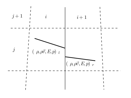
Figure 1: Reconstruction of conservative variables and pressure where discontinuity is introduced at the cell interface. The dashed lines represent the boundaries of the of the control volumes numbered by $i$ and $j$; the vertical solid line is the interface where the flux-splitting is performed. The discontinuity of the values and their slopes are depicted by oblique solid lines.

The last term in right-hand side of equation (9) is implemented to account for the SGS viscosity,

$$\mu_{sgs}=\rho(c_{\mu}\Delta)^{2}(2\vec{\sigma}:\vec{\sigma})^{1/2},$$ (10)

where $c_{\mu}$ is an adjustable constant, usually has the value: 0.1 $\sim$ 0.2, the filter width $\Delta$ is taken to be the local resolution, colon stands for the contract of tensor and $\vec{\sigma}=\partial_{i}v_{j}+\partial_{j}v_{i}$. Above model is called Smagorinsky model or sometimes Smagoringsky-Lilly model. In our calculations, the eddy viscosity is computed in the control volume by staggered mesh strategy and then interpolated to the cell interface. In the BGK scheme, there is intrinsic diffusion caused by particle collisions. In current study, we are only interested in the turbulent properties. So, the molecule Prandtl number $Pr$ is set very large. And the following diffusive flux (CS96) is implemented explicitly into the BGK scheme,

$$\vec{F}_{d}=-C_{T}\nabla T-C_{S}\nabla S,$$ (11)

where $S=C_{p}(\ln{T}-\nabla_{a}\ln{p})$ is the specific entropy, $C_{p}$ is the specific heat at constant pressure and $\nabla_{a}$ is the adiabatic gradient. In the stable layer, $C_{T}$ is set to make the diffusion carry out the input energy flux. In the convection zone, $C_{T}$ is very close to zero. $C_{S}=\mu_{sgs}/Pr_{sgs}$ represents the turbulent diffusion and is set to zero in the stale region, where $Pr_{sgs}$ is the effective Prandtl number of SGS turbulence and taken to be $1/3$.

3 Physical Models

Our physical problem is very similar to those studied by CS89 and CS96. An ideal gas ($p=\rho RT$) in a rectangular box is considered with gravity in the vertical direction. The side boundaries are periodic and the top and bottom boundaries are impenetrable and stress free. In order to avoid boundary effects, a very thin stable layer is placed below the upper boundary and the diffusive flux is gradually enhanced near the lower boundary to make it carry out total flux at the lower boundary. A constant energy flux $F_{b}=0.25$ is fed at the bottom. At the top, the entropy is fixed. The system is initially static:

$$T = (1+\mathcal{Z}(d-z)/d)T_{t},$$ (12)

$$\rho = (T/T_{t})^{n}\rho_{t},$$ (13)

$$p = (T/T_{t})^{n+1}p_{t},$$ (14)

$$g = (n+1)p_{t}\mathcal{Z}/(\rho_{t}d)$$ (15)

where $\mathcal{Z}=(T_{b}-T_{t})/T_{t}$ is the normalized parameter, $0\leq z\leq 1$ and $n$ is the polytropic gas index. The gravitational acceleration $g$ comes from the hydrostatic equilibrium $\partial p/\partial z=-\rho g$. The subscripts $t$ and $b$ denote top and bottom values respectively. Above solutions to Navier-Stokes equations are not stable against small perturbations. In all of our calculations, the velocity field is slightly perturbed initially. After long-time thermodynamic relaxation, the system will reach a statistical steady state. We defined a series of runs to test the effects of numerical parameters. The numerical effects of a variety of parameters were studied by Chan & Sofia ([1986], hereafter CS86) and CS89 in details. The effects of changing turbulent Prandtl number was tested by Singh & Chan([1993]). Here, we just focus on the important parameter $c_{\mu}$ in the SGS model and new parameter $C_{2}$ appearing in the BGK scheme. The details are given in the second line of Table 1.

All the cases we computed use a $29\times 29\times 45$ mesh. The vertical grid decreases smoothly with height (about $6$ grids per PSH) and the horizontal grid is uniform. The aspect ratio (width/depth) of the box is $1.5$.

4 Results

Figure 2: Distribution of temporally and horizontally averaged energy fluxes with depth. Dash dot line: diffusive flux; dotted line: kinetic energy flux; diamonds: enthalpy flux; solid line: total energy flux.

In this part, we show the results from the numerical simulations. All the runs were evolved $2000000$ numerical time-steps, corresponding to a dimensionless time around $858$, before the statistical analysis is performed. The statistical steady state is indicated by the balance of the input energy flux from the bottom and the outgoing energy flux through the top. In our calculations, the spatial variation of averaged total energy flux from $0.25$ is within $0.1\%$ (see solid line in Fig. 2). Another criterion is the averaged vertical mass flux which is less then $10^{-5}$ everywhere in all cases. Hence, the system will not undergo substantial adjustment any more. The statistical average covers $500000$ numerical time-steps.

Except for the instant velocity fields, all the other quantities investigated here are the mean values. For an arbitrary quantity $q$, $\langle q\rangle$ represents its combined horizontal and temporal mean, $q^{\prime}$ denotes the deviation from $\langle q\rangle$, $q^{\prime\prime}$ stands for the root mean square (rms) fluctuation from the $\langle q\rangle$.

In some figures, the integral pressure scale height (PSH) is shown by the vertical lines. For example, in Fig. 2, the vertical solid line denotes the location of stable-unstable interface near the upper boundary. The second dashed line at the left side of the solid line is 2 PSHs away from the upper stable-unstable interface. Although the numerical parameters are different for case A to case C, their relaxed thermal structure are nearly equivalent and the discrepancy between the integral PSH locations is very small. So, we can plot the results from all runs in the same figures.

4.1 Velocity Fields

Figure 3: Instant velocity fields at time $858$. Left: projection in vertical plane at $y=0.45$; right: projection in horizontal plane at $z=0.6$.

In CS86, the three-dimensional turbulent flow structure was well depicted by the pseudo stream lines. For sake of clarity, Fig. 3 shows the velocity fields projected in x-z plane and x-y plane. From the left panel of Fig.  3, it is evident to see that the high speed motions exist in the top region and are associated with the downward streams. In our calculations, the maximum Mach number $Ma$ occasionally exceeds one. In CS96, the SGS viscosity was enhanced by a factor $[1+0.5(v_{x}^{6}+v_{y}^{6}+v_{z}^{6})/c_{s}^{6}]$ to suppress the shocks occurring in the top region which would easily trigger the instability of the numerical computation, especially, during the early thermal relaxation. Based on flux-splitting (see Fig. 1), such implement can be avoided in gas-kinetic BGK scheme. If the nonlinear van Leer limiter is replaced by central interpolation, the supersonic motion cannot be handled correctly. Numerical tests also show that a $Ra$ less than $10^{9}$ will smooth the turbulence, the circulations become laminar. The solutions are almost unchanged when $Ra$ great than $10^{15}$. In current study, we adopt $Ra=10^{19}$. The networks of downward streams can be seen the right panel of Fig. 3.

4.2 Approximate Relations

Table 1: Quantitative Estimates of Some Approximate Relations.

Relation   Parameter	A	B	C	CS89	Deviation	ID	Category
$c_{\mu}$	0.2	0.25	0.2	0.2	(%)
$C_{2}$	1	1	0	- - -
$v^{\prime\prime}_{x}/v^{\prime\prime}_{z}$	0.69 ( 0.12 )	0.66 ( 0.11 )	0.62 ( 0.11 )	0.61 ( 0.05 )	8	R0†	III
$v^{\prime\prime}_{y}/v^{\prime\prime}_{z}$	0.57 ( 0.10 )	0.58 ( 0.10 )	0.64 ( 0.11 )	0.61 ( 0.05 )	2	R1	III
$(\rho^{\prime\prime}/\langle\rho\rangle)/(T^{\prime\prime}/\langle T\rangle)$	0.83 ( 0.01 )	0.83 ( 0.02 )	0.83 ( 0.01 )	0.89 ( 0.04 )	7	R2	I
$(p^{\prime\prime}/\langle p\rangle)/(T^{\prime\prime}/\langle T\rangle)$	0.57 ( 0.04 )	0.56 ( 0.04 )	0.57 ( 0.04 )	0.57 ( 0.07 )	1	R3	I
$S^{\prime\prime}/(C_{p}T^{\prime\prime}/\langle T\rangle)$	0.90 ( 0.01 )	0.90 ( 0.01 )	0.90 ( 0.01 )	0.94 ( 0.03 )	4	R4	I
$(p^{\prime\prime}/\langle p\rangle)/(v^{\prime\prime 2}/\langle T\rangle)$	0.48 ( 0.01 )	0.47 ( 0.01 )	0.48 ( 0.00 )	0.26 ( 0.01 )	83	R5‡	II
$p^{\prime\prime}/\langle\rho\rangle v^{\prime\prime 2}_{z}$	0.88 ( 0.14 )	0.85 ( 0.13 )	0.87 ( 0.14 )	0.51 ( 0.03 )	70	R6	IV
$T^{\prime\prime}/v^{\prime\prime 2}_{z}$	1.52 ( 0.15 )	1.51 ( 0.13 )	1.51 ( 0.15 )	0.90 ( 0.10 )	68	R7	IV
$C(T^{\prime},S^{\prime})$	0.98 ( 0.00 )	0.98 ( 0.02 )	0.98 ( 0.03 )	0.99 ( 0.01 )	1	R8	I
$C(\rho^{\prime},S^{\prime})$	-0.93 ( 0.01 )	-0.92 ( 0.01 )	-0.92 ( 0.01 )	-0.89 ( 0.06 )	4	R9	I
$C(\rho^{\prime},T^{\prime})$	-0.83 ( 0.02 )	-0.83 ( 0.02 )	-0.82 ( 0.03 )	-0.82 ( 0.05 )	1	R10	I
$C(p^{\prime},T^{\prime})$	0.59 ( 0.04 )	0.59 ( 0.04 )	0.59 ( 0.03 )	0.49 ( 0.05 )	20	R11	II
$C(v_{z},T^{\prime})$	0.78 ( 0.02 )	0.79 ( 0.02 )	0.77 ( 0.02 )	0.81 ( 0.03 )	4	R12	I
$C(v_{z},S^{\prime})$	0.76 ( 0.02 )	0.78 ( 0.03 )	0.75 ( 0.02 )	0.81 ( 0.03 )	6	R13	I
$C(v_{z},\rho^{\prime})$	-0.64 ( 0.01 )	-0.67 ( 0.01 )	-0.63 ( 0.01 )	-0.74 ( 0.03 )	13	R14	II
$\langle v_{z}\rho^{\prime}\rangle/\langle v_{z}\rangle\langle\rho\rangle$	-1.00 ( 0.02 )	-0.99 ( 0.02 )	-1.00 ( 0.02 )	-1.00 ( - - - )	0	R15	I
$\langle v_{z}p\rangle/\langle v_{z}\rangle\langle p\rangle$	1.49 ( 0.06 )	1.44 ( 0.05 )	1.50 ( 0.06 )	1.24 ( 0.08 )	19	R16	II
$\langle v_{z}T^{\prime}\rangle/\langle v_{z}\rangle\langle T\rangle$	1.46 ( 0.06 )	1.41 ( 0.06 )	1.46 ( 0.06 )	1.26 ( 0.08 )	15	R17	II
$\langle v_{z}S^{\prime}\rangle/C_{p}\langle v_{z}\rangle$	1.28 ( 0.05 )	1.24 ( 0.04 )	1.28 ( 0.05 )	1.20 ( 0.08 )	6	R18	I
$\langle v_{z}\rangle/\langle{v^{\prime\prime}}_{z}^{3}\rangle\langle T\rangle$	0.81 ( 0.08 )	0.85 ( 0.07 )	0.80 ( 0.09 )	0.58 ( 0.07 )	41	R19	IV
$F_{ep}/C_{p}\langle p\rangle\langle v_{z}\rangle$	1.49 ( 0.06 )	1.44 ( 0.05 )	1.50 ( 0.06 )	1.25 ( 0.08 )	18	R20	II
$F_{ep}/C_{p}\langle\rho\rangle{v^{\prime\prime}}_{z}^{3}$	1.20 ( 0.15 )	1.23 ( 0.13 )	1.20 ( 0.15 )	0.72 ( 0.06 )	68	R21	IV
$T^{\prime\prime}/\langle T\rangle=a\Delta\nabla+b$	$a=1.92$	$a=1.88$	$a=1.95$	$a=1.05$	83	R22	II
	$b=0.0029$	$b=0.0025$	$b=0.0030$	$b=0.0027$
	( $0.0004^{\ast}$ )	( $0.0001^{\ast}$ )	( $0.0002^{\ast}$ )	( $0.0008^{\ast}$ )
$v^{\prime\prime}/\langle T\rangle=a\Delta\nabla+b$	$a=1.01$	$a=1.03$	$a=1.03$	$a=1.17$	13	R23	II
	$b=0.0027$	$b=0.0023$	$b=0.0028$	$b=0.0032$
	( $0.0004^{\ast}$ )	( $0.0002^{\ast}$ )	( $0.0004^{\ast}$ )	( $0.0008^{\ast}$ )
$\Delta\nabla=a[F_{b}/(0.8C_{p}\langle p\rangle\langle T\rangle^{1/2})]^{2/3}+b$	$a=0.71$	$a=0.71$	$a=0.70$	$a=0.9$	21	R24	II
	$b=-0.0013$	$b=-0.0011$	$b=-0.0013$	$b=-0.002$
	( $0.0002^{\ast}$ )	( $0.0002^{\ast}$ )	( $0.0001^{\ast}$ )	( $0.0008^{\ast}$ )

• New relation defined in current paper.

• ${v^{\prime\prime}}^{2}={v^{\prime\prime}}_{x}^{2}+{v^{\prime\prime}}_{y}^{2}+{v^{\prime\prime}}_{z}^{2}$.

• These are standard deviations of the least-squares fits.

Our BGK code has been extensively tested for laminar flows (Tian et al. [2007]). In order to validate the incorporation of SGS model, we re-estimate quantitatively some approximate relations among the thermodynamic variables and their fluctuations. The results are given in Table 1 where the results from CS89 are also listed for comparison. Our computational models are partially similar to CS89 and partially to CS96. Models of CS89 undergo substantially adjustment near the boundaries and we cannot afford the high-resolution desired in CS96. During the data analysis, the correlation function of quantity $q$ and $p$ is defined as $C[q,p]=\langle qp\rangle/({\langle q^{2}\rangle^{1/2}}{\langle p^{2}\rangle^{1/2}})$. The standard deviations of these approximations ($\sigma_{1}$) are given in the brackets. The deviation of $Ri$ from CS89 is calculated by $\sigma_{2}=|((Ri_{A}+Ri_{B}+Ri_{C})/3-Ri_{CS89})/Ri_{CS89}|$. We only concentrate on the middle region in the convection zone, namely, 1 PSH from the bottom and 2 PSHs from the upper stable-unstable interface. The investigated layer expands about 3 PSHs.

Figure 4: Height distributions of fluctuations and relative fluctuations for case C. Left: $p^{\prime\prime}/\langle{p}\rangle$ (solid line), $T^{\prime\prime}/\langle{T}\rangle$ (dotted line), $\rho^{\prime\prime}/\langle{\rho}\rangle$ (dashed line); right: $v^{\prime\prime}_{x}$ (dashed line), $v^{\prime\prime}_{y}$ (dotted line), $v^{\prime\prime}_{z}$ (solid line).

The approximate relations and correlations in Table 1 are classified roughly into four categories which are indicated by Roman numerals in the last column according to the goodness of fit and discrepancy from CS89. These categories are: Category I: $\sigma_{1}\leq 0.6$ and $\sigma_{2}\leq 10$%; Category II: $\sigma_{1}\leq 0.6$ and $\sigma_{2}>10$%; Category III: $\sigma_{1}>0.6$ and $\sigma_{2}\leq 10$%; Category IV: $\sigma_{1}>0.6$ and $\sigma_{2}>10$%.

Category I contains the best relations where the thermal variables are mainly involved, i.e. $\rho$, $p$, $T$ and their fluctuations. These relations should be weekly affected by numerical scheme and details of the computational models. In the work of Kim et al. ([1995]) where a realistic equation of state (EOS) was used, these relations are different from current studies. Therefore, Category I may be dominantly determined by EOS.

Most relations of Category II are functions of pressure $p$ , velocity $\vec{v}$ and their fluctuations. The amplitude of the fluctuations of the components of velocity in our computation is lower than those in CS89 (Fig. 1 therein) and CS96 (Fig. 2 therein) while the amplitude of the relative fluctuations of thermal quantities are around two times larger than those in CS89 (see Fig. 2 therein) and in Singh’s work ([1993]). Hence when the fluctuations of thermal variables are expressed in terms of $v^{\prime\prime}$, $v^{\prime\prime}_{z}$, etc., the coefficients are nearly doubled, e.g., $R5$ and $R22$. This can also be seen in Fig. 3a in CS96.

Ratios of $v^{\prime\prime}_{x}/v^{\prime\prime}_{z}$ and $v^{\prime\prime}_{y}/v^{\prime\prime}_{z}$ do not deviate from CS89 very much, but the fitting is not accurate. This may be caused by the effects of the boundary and transition layers. It is obvious from Fig. 4 that the height distribution of $v^{\prime\prime}_{z}$ is not flat as CS89. There is a small hump below the upper transition layer (one PHS from the unstable-stable interface) which can also be found in CS96. We believe that the unstable-stable transition is responsible for this. The large difference in Category IV should be caused by the high order powers of velocity fluctuations.

$R22$ $\sim$ $R24$ are commonly approximated in MLT. In current study, these relations are fitted by linear approximation very well. However, the slopes are different from the CS86 and CS96. The situation of $R22$ can be explained as above. For $R23$, the reasons may lie in the fact that in the upper convective region, the amplitude of $v^{\prime\prime}_{z}$ from CS96 is larger than ours and therefor we need a smaller $R23$. CS96 got a smaller $R24$ (0.78) than CS89. In current study, it is even smaller which implies a smaller super-adiabatic gradient $\Delta\nabla$.

The cause of most of the discrepancies between current study and CS89 may be the larger $T^{\prime\prime}$ and smaller $v_{z}^{\prime\prime}$. In the traditional theory of stellar convection, the enthalpy flux is proportional to the fluctuations of temperature and velocity, i.e., $F_{e}\sim C_{p}v^{\prime\prime}T^{\prime\prime}$ and the kinetic flux is totally neglected. When the kinetic flux is comparable to the total flux, this kind of proportional relation is not exactly held any more. Based on the following facts:

1. $F_{b}=0.0625$, $\max{T^{\prime\prime}}\sim 0.022$, $\max{v^{\prime\prime}_{z}}\sim 0.2$ (Singh [1993], Fig. 1 and Fig. 5);

2. $F_{b}=0.1250$, $\max{T^{\prime\prime}}\sim 0.023$, $\max{v^{\prime\prime}_{z}}\sim 0.22$ (CS89, Fig. 1 and Fig. 2);

3. $F_{b}=0.2500$, $\max{T^{\prime\prime}}\sim 0.065$, $\max{v^{\prime\prime}_{z}}\sim 0.35$ (CS96, Fig. 2);

4. $F_{b}=0.2500$, $\max{T^{\prime\prime}}\sim 0.078$, $\max{v^{\prime\prime}_{z}}\sim 0.23$ (current, Fig. 4);

5. $F_{b}=0.6551$, $\max{T^{\prime\prime}}\sim 0.129$, $\max{v^{\prime\prime}_{z}}\sim 0.27$ (Kim [1995], Fig. 7 and Fig. 8),

we can conclude that the $T^{\prime\prime}$ and $v_{z}^{\prime\prime}$ are proportional to $F_{b}$ in a nonlinear way. Note that current study use a different numerical scheme and Kim adopted a realistic EOS. It is beyond the scope of current study to perform a quantitative analysis of such relations.

Above comparison shows that the dynamical properties and thermal properties for stellar type of convection may be affected by different aspects of the numerical models separately. Thermal structure is mainly determined by physical parameters while dynamic motions can easily affected by numerical parameters.

Figure 5: Height distributions of natural logarithm of $\chi$, $V$ and $Z$. Solid line: case A; dotted line: case B; dashed line: case C.

4.3 Anisotropic Turbulence

Xiong’s non-local time-dependent stellar convection theory is based on Reynolds stress method. It is dynamic theory of auto- and cross-correlation functions of turbulent velocity and temperature fluctuations. These fluctuations are defined as the derivation from the density weighted average, i.e.,

$$u^{\prime}_{i}=v_{i}-\frac{\langle\rho v_{i}\rangle}{\langle\rho\rangle},\quad\tilde{T}^{\prime}=T-\frac{\langle\rho T\rangle}{\langle\rho\rangle}.$$ (16)

The start point of Xiong’s theory is a set of partial differential equations of

$$\chi^{2}=\langle{w^{\prime}_{i}w^{\prime i}}\rangle/3,\quad Z=\langle{\tilde{T}^{\prime 2}}\rangle/\langle{\tilde{T}}\rangle^{2},\quad V=\langle{\tilde{T}^{\prime}w^{\prime}_{i}}\rangle/\langle{\tilde{T}}\rangle,$$ (17)

where $w^{\prime}_{i}=\rho u^{\prime}_{i}/\langle{\rho}\rangle$, $\langle{\tilde{T}}\rangle={\langle\rho T\rangle}/{\langle\rho\rangle}$ and the summation convention is adopted. The numerical results of $\chi$, $Z$ and $V$ are given in Fig. 5. In the closure models of Xiong’s theory, three adjustable parameters, i.e., $c_{1}$, $c_{2}$ and $c_{3}$ are introduced. $c_{3}$ is used to describe the anisotropic turbulent motions. In Deng’s ([2006]) work, $c_{3}$ was related to turbulent velocity by ${w^{\prime}}_{z}^{2}/({w^{\prime}}_{x}^{2}+{w^{\prime}}_{y}^{2})=(3+c_{3})/2c_{3}$ in the fully unstable zone. In the upper overshooting region, they proposed that ${w^{\prime}}_{z}^{2}/({w^{\prime}}_{x}^{2}+{w^{\prime}}_{y}^{2})\sim 0.5$ and is independent of $c_{3}$. In the lower overshooting zone, ${w^{\prime}}_{z}^{2}/({w^{\prime}}_{x}^{2}+{w^{\prime}}_{y}^{2})\leq 0.5$ and decrease as $c_{3}$ decrease. There is no enough room for overshooting in our models. The ratio of ${w^{\prime}}_{z}^{2}/({w^{\prime}}_{x}^{2}+{w^{\prime}}_{y}^{2})$ from numerical simulations is given in Fig. 6 from which we can see this ratio is slightly dependent on $c_{\mu}$ and $C_{2}$. In the upper efficient-inefficient convection interface (about 1 PSH from unstable-stable interface), this value approximately equals to $0.5$. It takes its maximum at the location where the turbulent convection starts to become inefficient near the bottom. Its maximum is affected evidently by $c_{\mu}$ and $C_{2}$. Current study cannot give a definite solution for anisotropic turbulence. Here, we present preliminary suggestions. Suppose that ${w^{\prime}}_{z}^{2}/({w^{\prime}}_{x}^{2}+{w^{\prime}}_{y}^{2})=(3+c_{3})/2c_{3}$ is held in current models, we can conclude that $c_{3}$ is infinitely large at the upper efficient-inefficient interface and decreases as the distance from the boundaries increases. The minimum of $c_{3}$ is about $0.75$.

Figure 6: Height distribution of ${w^{\prime}}_{z}^{2}/({w^{\prime}}_{x}^{2}+{w^{\prime}}_{y}^{2})$. Solid line: case A; dotted line: case B; dashed line: case C.

4.4 Non-local Transport Models

Figure 7: (a) Non-local turbulent transports (in common logarithm). (b)$\sim$(d) The approximate coefficients. Solid line: case A; dotted line: case B; dashed line: case C.

Generally, a Reynolds stress method suffers the so-called closure problem. CS96 numerically studied the popular closures and found they were poor. Some third order moments representing the non-local transport effects were approximated by gradient models in Xiong’s work ([1989]), i.e.,

$$NLT1 = \langle{u^{\prime}_{k}w^{\prime}_{i}w^{\prime i}}\rangle=-\chi l_{1}\nabla_{k}\langle{w^{\prime}_{i}w^{\prime i}}\rangle,$$ (18)

$$NLT2 = \langle{u^{\prime}_{k}\tilde{T}^{\prime 2}}\rangle/\langle{\tilde{T}}\rangle^{2}=-\chi l_{3}\nabla_{k}(\langle{\tilde{T}^{\prime 2}}\rangle/\langle{\tilde{T}}\rangle^{2}),$$ (19)

$$NLT3 = \langle{u^{\prime}_{k}w^{\prime i}\tilde{T}^{\prime}}\rangle/\langle{\tilde{T}}\rangle=-\chi l_{5}\nabla_{k}(\langle{w^{\prime i}\tilde{T}^{\prime}}\rangle/\langle{\tilde{T}}\rangle),$$ (20)

with $l_{1}\simeq l_{3}\simeq l_{5}=\Lambda$, where $\Lambda$ is the Lagrangian integral length scale of turbulence. The non-local transports and coefficients from numerical simulations for all cases are shown in Fig. 7 . From panel (a) of Fig. 7, we can see that the $|\langle{u^{\prime}_{k}w^{\prime}_{i}w^{\prime i}}\rangle|$ is about one order larger than $|\langle{u^{\prime}_{k}w^{\prime i}\tilde{T}^{\prime}}\rangle/\langle{T}\rangle|$ and $|\langle{u^{\prime}_{k}\tilde{T}^{\prime 2}}\rangle/\langle{T}\rangle^{2}|$ is three orders less than $|\langle{u^{\prime}_{k}w^{\prime i}\tilde{T}^{\prime}}\rangle/\langle{T}\rangle|$. Hence, the non-local transports are dominated by turbulent kinetic energy. Panel (b)$\sim$(d) of Fig. 7 show that the $l_{1}$, $l_{3}$ and $l_{5}$ gradually increase with the distance from the top boundary and change this trend near the interface where the turbulent convection become inefficient. The variation of $l_{1}$ is slow in the lower half convection zone around the value of 1.8. But it is affected by $c_{\mu}$ and $C_{2}$ obviously. $l_{5}$ is about ten times larger than $l_{3}$. Both of $l_{3}$ and $l_{5}$ vary rapidly which suggests that there may not exist the universal constant for these closure models.

4.5 Effects of Numerical Parameters: $c_{\mu}$ and $C_{2}$

Figure 8: Comparison of auto-correlations of the vertical velocity. Solid line: case A; dotted line: case B; dashed line: case C. $p_{i}$ is the pressure at the unstable-stable interface.

In current LES, the local effective grid Reynolds number is enlarged by SGS model whose amplitude is controlled by Deardorff constant $c_{\mu}$. An inadequately small $c_{\mu}$ would cause the building-up of the kinetic energy at the two-grid level and make the computation crashed. If $c_{\mu}$ is too large, the turbulent motions will be damped down. The proper value of $c_{\mu}$ is resolution- and method-dependent since the numerical dissipation also plays an important role in the behavior of turbulence. Deardorff ([1971]) suggested a value of $0.2$ for $c_{\mu}$ which was used in the CS89. In CS96, this value was increased to $0.25$.

In the flux-splitting method, the discontinuity is introduced at the cell interface (see Fig. 1) by limiters. Additional dissipation (the second term in the left hand side of equation (9)) is employed to handle the strong shock waves near the sharp jumps of pressure. The typical value of $C_{2}$ is 1. In the smooth region this kind of discontinuity should be very small. However, our simulations have lower resolution and the computing zone extends about seven PSHs. So it is necessary to check if these values are adequate for studying the stellar type of convection.

Relations $R2$ $\sim$ $R4$ and $R9$ $\sim$ $R11$ in Table 1 show that the effects of changing these parameters on the thermal structure are really slight. They both affect the eddy properties with very small amplitude which can be seen from Fig. 8 where the auto-correlations of the vertical velocity are shown. Their profiles are nearly symmetrical except in the upper stable and transition zone. The half width at half maximum (HWHM) of these profiles should be sensitive on the viscosity (CS86). $R0$ and $R1$ in Table 1 are the $v^{\prime\prime}_{x}/v^{\prime\prime}_{z}$ and $v^{\prime\prime}_{y}/v^{\prime\prime}_{z}$, respectively. They should be nearly equal to each other for isotropic turbulent flows. In our study, for case A ($c_{\mu}=0.2$, $C_{2}=1$), the discrepancy between them is clear which becomes slight for case B ($c_{\mu}=0.25$, $C_{2}=1$) and further slight for case C ($c_{\mu}=0.2$, $C_{2}=0$). This kind of anisotropy comes from the initially perturbation and can also bee found in Fig.7 and Fig.11 in CS86. So it seems that $c_{\mu}=0.25$ is more suitable for current study. In the deep stellar convection, the shock waves are mild. Hence, the flux-splitting may enough to handle it as in our tests. We suggest that it is better to make $C_{2}$ as small as possible because it would enhance the anisotropy which can be diminished by larger $c_{\mu}$.

5 Conclusions

In this paper, we present a preliminary application of gas-kinetic BGK scheme to the simulation of turbulent convection in stellar atmosphere. The approximate relations among thermodynamic variables, their fluctuations and correlations were examined. The anisotropy and diffusive models of non-local transport were investigated too. The effects of varying numerical parameters were also tested. The main conclusions are summarized as follows:

1. The behavior of the thermal variables and dynamic variables are affected by different aspects of the models and numerical scheme. For example, the fluctuations of density and pressure are dominantly determined by physical models while the fluctuations of velocity are sensitively dependent on numerical parameters, e.g., $c_{\mu}$ and $C_{2}$.

2. There is no constant ratio of $w^{\prime\prime}_{z}/(w^{\prime\prime}_{x}+w^{\prime\prime}_{y})$ for anisotropic turbulence in current models. We suggest that $c_{3}$ take an infinite value at the boundary and approach its minimum ($0.75$) in the deep convective region.

3. The diffusive models for non-local transport are not applicable since the coefficients for different quantities are dramatically different. The best situation is the turbulent transport of turbulent kinetic energy where a roughly flat region exists for $l_{1}$.

4. For current resolutions, $c_{\mu}=0.25$ is better than $c_{\mu}=0.2$. And $C_{2}$ should be set as small as possible in any cases. A flux-splitting technique is needed to stabilized the shock waves near the top. A Rayleigh number less than $10^{9}$ may smear the turbulent motions.

Our simulations may suffer from the lower resolutions, aspect ratio and the number of testing cases. But it is enough for the purpose of validation and get some preliminary results. A further study will be performed in the future.