Analysis of regular inflationary cosmological models with two torsion functions in Poincaré gauge theory of gravity

Abstract

Analysis of regular inflationary cosmological models with two torsion functions filled with scalar field with quadratic potential and ultrarelativistic matter is carried out numerically. Properties of different stages of regular inflationary cosmological solutions are studied, restrictions on admissible values of parameters and initial conditions at transition from compression to expansion are found. The structure of extremum surface in space of physical variables is investigated.

,

1 Introduction

As it was shown in a number of papers (see [1-5] and references herein), the Poincaré gauge theory of gravity (PGTG) offers opportunities to solve some principal problems of general relativity theory (GR) and modern cosmology. It is because the gravitational interaction in the framework of PGTG can have the repulsive character under certain physical conditions in usual gravitating systems with positive values of energy density and pressure. As a result the PGTG allows to build totally regular Big Bang scenario with an accelerating stage of cosmological expansion at present epoch. Such scenario is based on homogeneous isotropic models (HIM) with two torsion functions built in the framework of PGTG in our previous paper [4], where as an example a particular regular inflationary cosmological solution was obtained by numerical calculations.

The present paper is devoted to analysis of regular inflationary cosmological HIM with two torsion functions in the PGTG. In Section 2 cosmological equations for such models in dimensionless form are given. In Section 3 the most important general properties of regular inflationary cosmological solutions are analyzed numerically. In Section 4 we study extremum surfaces, on which the Hubble parameter vanishes and initial conditions for investigated solutions are given.

2 Cosmological equations for HIM with two torsion functions in dimensionless form

In the framework of PGTG any HIM is described by three geometric characteristics: the scale factor of Robertson-Walker metrics $R$ and two torsion functions $S_{1}$ and $S_{2}$ as functions of time $t$. By using general form of gravitational Lagrangian including both a scalar curvature and various invariants quadratic in gravitational field strengths — curvature and torsion tensors, cosmological equations for HIM with two torsion functions were deduced in [4]. The energy density $\rho$ and pressure $p$ of gravitating matter play the role of sources of gravitational field in cosmological equations. These equations contain three indefinite parameters: parameter $\alpha$ with inverse dimension of energy density determining the scale of extremely high energy densities, parameter $b$ with dimension of parameter $f_{0}=(16\pi G)^{-1}$ ($G$ is Newton’s gravitational constant, the light velocity $c=1$) and dimensionless parameter $\varepsilon$. As was shown in [4], by certain restrictions on indefinite parameters cosmological equations for HIM lead to observable accelerating cosmological expansion at present epoch. According to obtained estimations the parameter $b$ has to be close to $f_{0}$ and the parameter $\varepsilon$ satisfies the following conditions $0<\varepsilon\ll 1$.

In order to analyze inflationary cosmological solutions we will consider HIM filled with scalar field $\phi$ with a potential $V$ and usual gravitating matter (values of gravitating matter are denoted by means of index “${m}$”). In this case we have:

$$\rho=\frac{1}{2}\left(\frac{\partial\phi}{\partial t}\right)^{2}+V+\rho_{m}\quad(\rho>0),\quad p=\frac{1}{2}\left(\frac{\partial\phi}{\partial t}\right)^{2}-V+p_{m}.$$

To investigate inflationary solutions we transform cosmological equations obtained in [4] to dimensionless form by introducing dimensionless units for all variables and parameter $b$ entering these equations and denoted by means of  $\tilde{}$  by the following way:

$$\begin{array}[]{lcl}t\to\tilde{t}=t/\sqrt{6f_{0}\alpha},&&R\to\tilde{R}=R/\sqrt{6f_{0}\alpha},\\ \rho\to\tilde{\rho}=\alpha\,\rho,&&p\to\tilde{p}=\alpha\,p,\\ \phi\to\tilde{\phi}=\phi/\sqrt{6f_{0}},&&b\to\tilde{b}=b/f_{0},\\ H\to\tilde{H}=H\sqrt{6f_{0}\alpha},&&S_{1,2}\to\tilde{S}_{1,2}=S_{1,2}\sqrt{6f_{0}\alpha}.\end{array}$$ (1)

where dimensionless Hubble parameter $\tilde{H}$ is defined by usual way $\tilde{H}=\tilde{R}^{-1}\frac{d\tilde{R}}{d\tilde{t}}$. Numerical analysis in Section 3 will be made by choosing quadratic potential $V=\frac{1}{2}m^{2}\phi^{2}$, then in accordance with (1) the transition to dimensionless units gives:

$$V\to\tilde{V}=\alpha V,\qquad\tilde{V}=\frac{1}{2}\tilde{m}^{2}\tilde{\phi}^{2},\qquad m\to\tilde{m}=m\sqrt{6f_{0}\alpha}.$$

Because of the transformation (1) cosmological equations ((22)–(23) in [4]) take the following dimensionless form, where the differentiation with respect to dimensionless time $\tilde{t}$ is denoted by means of the prime and the sign of  $\tilde{}$  is omitted below:

$$\frac{k}{R^{2}}+(H-2S_{1})^{2}=\frac{1}{Z}\left[{\rho+\left(Z-b\right)S_{2}^{2}+\frac{1}{4}\left({\rho-3p-12bS_{2}^{2}}\right)^{2}}\right]$$

$$-\frac{\varepsilon}{2Z}\left[{\left({HS_{2}+S_{2}^{\prime}}\right)^{2}+4\left({\frac{k}{{R^{2}}}-S_{2}^{2}}\right)S_{2}^{2}}\right],$$ (2)

$$H^{\prime}+H^{2}-2HS_{1}-2S_{1}^{\prime}=-\frac{1}{2Z}\left[\rho+3p-\frac{1}{2}\left({\rho-3p-2bS_{2}^{2}}\right)^{2}\right]$$

$$-\frac{\varepsilon}{Z}\left({\rho-3p-2bS_{2}^{2}}\right)S_{2}^{2}+\frac{{\varepsilon}}{2Z}\left[{\left({HS_{2}+S_{2}^{\prime}}\right)^{2}+4\left({\frac{k}{{R^{2}}}-S_{2}^{2}}\right)S_{2}^{2}}\right],$$ (3)

($Z\equiv 1+\rho-3p-2\left({b+\varepsilon}\right)S_{2}^{2}=1+4V-\phi^{\prime 2}+\rho_{\mathrm{m}}-3p_{\mathrm{m}}-2\left({b+\varepsilon}\right)S_{2}^{2}$). The torsion function $S_{1}$ in dimensionless form entering (2)–(3) is

$$S_{1}=-\frac{3}{4Z}\left[2\frac{\partial V}{\partial\phi}\phi^{\prime}\ +H\left({Y+2\phi^{\prime 2}}\right)-\frac{2}{3}\left({2b-\varepsilon}\right)S_{2}\,S_{2}^{\prime}\right],$$ (4)

where

$$Y\equiv\left(\rho_{\mathrm{m}}+p_{\mathrm{m}}\right)\left(3\frac{dp_{\mathrm{m}}}{d\rho_{\mathrm{m}}}-1\right)+2\varepsilon S_{2}^{2}$$

and dimensionless torsion function $S_{2}$ satisfies the following differential equation of the second order:

$$\varepsilon\left[S_{2}^{\prime\prime}+3HS_{2}^{\prime}+3H^{\prime}S_{2}-4\left(S_{1}^{\prime}-3HS_{1}+4S_{1}^{2}\right)S_{2}\right]$$

$$-2\left({\rho-3p-2bS_{2}^{2}}\right)S_{2}-2\left({1-b}\right)S_{2}=0\,.$$ (5)

By using dimensionless units the equation for scalar field and conservation law for gravitating matter have the usual form

$$\phi^{\prime\prime}+3H\phi^{\prime}=-\frac{\partial V}{\partial\phi}\,,$$ (6)

$$\rho_{m}^{\prime}+3H\left(\rho_{\mathrm{m}}+p_{\mathrm{m}}\right)=0.$$ (7)

By means of (6)–(7) and (4) for $S_{1}$-function we can transform cosmological equations (2)–(3) and (5) for $S_{2}$-function to the following form:

$$H^{2}\left\{\left[Z+\frac{3}{2}\left(Y+2\phi^{\prime}\right)\right]^{2}+\frac{1}{2}\varepsilon S_{2}^{2}Z\right\}$$

$$+6H\left\{\left[Z+\frac{3}{2}\left(Y+2\phi^{\prime 2}\right)\right]\times\left[\frac{\partial V}{\partial\phi}\phi^{\prime}-\frac{1}{3}\left(2b-\varepsilon\right)S_{2}S_{2}^{\prime}\right]+\varepsilon S_{2}S_{2}^{\prime}Z\right\}$$

$$+9\left[\frac{\partial V}{\partial\phi}\phi^{\prime}-\frac{1}{3}\left(2b-\varepsilon\right)S_{2}S_{2}^{\prime}\right]^{2}+\frac{1}{2}\varepsilon\left[S_{2}^{\prime 2}+4\left(\frac{k}{R^{2}}-S_{2}^{2}\right)S_{2}^{2}\right]Z$$

$$-\left[\rho_{\mathrm{m}}+\frac{1}{2}\phi^{\prime}+V-bS_{2}^{2}+\frac{1}{4}\left(\rho_{\mathrm{m}}-3p_{\mathrm{m}}+4V-\phi^{\prime 2}-2bS_{2}^{2}\right)^{2}\right]Z$$

$$+\left(\frac{k}{R^{2}}-S_{2}^{2}\right)Z^{2}=0,$$ (8)

$$H^{\prime}\left[1+\frac{3}{2Z}\left(Y+2\phi^{\prime 2}\right)\right]+H^{2}\left\{1+\frac{3}{2Z}\left(Y+2\phi^{\prime 2}\right)-\frac{9}{2Z^{2}}\left(Y+2\phi^{\prime 2}\right)\left(Y+2\phi^{\prime 2}-2\varepsilon S_{2}^{2}\right)\right.$$

$$\left.-\frac{9}{2Z}\left[3\frac{d^{2}p_{\mathrm{m}}}{d\rho_{\mathrm{m}}^{2}}\left(\rho_{\mathrm{m}}+p_{\mathrm{m}}\right)^{2}+\left(3\frac{dp_{\mathrm{m}}}{d\rho_{\mathrm{m}}}-1\right)\left(1+\frac{dp_{\mathrm{m}}}{d\rho_{\mathrm{m}}}\right)\left(\rho_{\mathrm{m}}+p_{\mathrm{m}}\right)+4\phi^{\prime 2}\right]\right\}$$

$$-\frac{3}{Z}H\left\{\left[4\frac{\partial V}{\partial\phi}\phi^{\prime}+\frac{1}{3}\left(2b-7\varepsilon\right)S_{2}S_{2}^{\prime}\right]+\frac{3}{Z}\left[\left(\frac{\partial V}{\partial\phi}\phi^{\prime}-\frac{1}{3}\left(2b-\varepsilon\right)S_{2}S_{2}^{\prime}\right)\right.\right.$$

$$\left.\left.\times\left(Y+2\phi^{\prime 2}-2\varepsilon S_{2}^{2}\right)+\left(Y+2\phi^{\prime 2}\right)\times\left(\frac{\partial V}{\partial\phi}\phi^{\prime}-\frac{2}{3}\left(b+\varepsilon\right)S_{2}S_{2}^{\prime}\right)\right]\right\}$$

$$+\frac{3}{Z}\left\{\frac{\partial^{2}V}{\partial\phi^{2}}\phi^{\prime 2}-\left(\frac{\partial V}{\partial\phi}\right)^{2}\right.$$

$$\left.-\frac{6}{Z}\left(\frac{\partial V}{\partial\phi}\phi^{\prime}-\frac{1}{3}\left(2b-\varepsilon\right)S_{2}S_{2}^{\prime}\right)\times\left(\frac{\partial V}{\partial\phi}\phi^{\prime}-\frac{2}{3}\left(b+\varepsilon\right)S_{2}S_{2}^{\prime}\right)\right.$$

$$\left.-\frac{1}{3}\left(2b-\varepsilon\right)\left(S_{2}^{\prime 2}+S_{2}S_{2}^{\prime\prime}\right)\right\}$$

$$=-\frac{1}{2Z}\left[\rho_{\mathrm{m}}+3p_{\mathrm{m}}-2\left(V-\phi^{\prime 2}\right)-\frac{1}{2}\left(\rho_{\mathrm{m}}-3p_{\mathrm{m}}+4V-\phi^{\prime 2}-2bS_{2}^{2}\right)^{2}\right]$$

$$-\frac{\varepsilon}{Z}\left(\rho_{\mathrm{m}}-3p_{\mathrm{m}}+4V-\phi^{\prime 2}-2bS_{2}^{2}\right)S_{2}^{2}$$

$$+\frac{\varepsilon}{2Z}\left[\left(HS_{2}^{2}+S^{\prime 2}\right)^{2}+4\left(\frac{k}{R^{2}}-S_{2}^{2}\right)S_{2}^{2}\right],$$ (9)

$$S_{2}^{\prime\prime}\left[1-\frac{2}{Z}\left(2b-\varepsilon\right)S_{2}^{2}\right]+3H^{\prime}S_{2}\left[1+\frac{1}{Z}\left(Y+2\phi^{\prime 2}\right)\right]+3HS_{2}^{\prime}$$

$$-\frac{9}{Z}H^{2}S_{2}\left[Y+6\phi^{\prime 2}+3\frac{d^{2}p_{\mathrm{m}}}{d\rho_{\mathrm{m}}^{2}}\left(\rho_{\mathrm{m}}+p_{\mathrm{m}}\right)^{2}\right.$$

$$\left.+\left(3\frac{dp_{\mathrm{m}}}{d\rho_{\mathrm{m}}}-1\right)\left(1+\frac{dp_{\mathrm{m}}}{d\rho_{\mathrm{m}}}\right)\left(\rho_{\mathrm{m}}+p_{\mathrm{m}}\right)+\frac{1}{Z}\left(Y+2\phi^{\prime 2}\right)\right.$$

$$\left.\vphantom{\frac{dp_{\mathrm{m}}}{d\rho_{\mathrm{m}}}}\times\left(Y+2\phi^{\prime 2}-2\varepsilon S_{2}^{2}\right)\right]-3HS_{2}\left\{\frac{4}{Z}\left(4\frac{\partial V}{\partial\phi}\phi^{\prime}-\frac{1}{2}\left(2b+\varepsilon\right)S_{2}S_{2}^{\prime}\right)\right.$$

$$\left.+\frac{6}{Z^{2}}\left[\left(\frac{\partial V}{\partial\phi}\phi^{\prime}-\frac{1}{3}\left(2b-\varepsilon\right)S_{2}S_{2}^{\prime}\right)\left(Y+2\phi^{\prime 2}-2\varepsilon S_{2}S_{2}^{\prime}\right)\right.\right.$$

$$\left.\left.-\left(Y+2\phi^{\prime 2}\right)\left(\frac{\partial V}{\partial\phi}\phi^{\prime}-\frac{2}{3}\left(b+\varepsilon\right)S_{2}S_{2}^{\prime}\right)\right]\right\}$$

$$-\frac{9}{Z^{2}}S_{2}\left[H\left(Y+2\phi^{\prime 2}\right)+2\left(\frac{\partial V}{\partial\phi}\phi^{\prime}-\frac{1}{3}\left(2b-\varepsilon\right)S_{2}S_{2}^{\prime}\right)\right]^{2}$$

$$-\frac{6}{Z}S_{2}\left[\left(\frac{\partial V}{\partial\phi}\right)^{2}-\frac{\partial^{2}V}{\partial\phi^{2}}\phi^{\prime 2}+\frac{1}{3}\left(2b-\varepsilon f_{0}\right)S_{2}^{\prime 2}\right.$$

$$\left.+\frac{6}{Z}\left(\frac{\partial V}{\partial\phi}\phi^{\prime}-\frac{1}{3}\left(2b-\varepsilon\right)S_{2}S_{2}^{\prime}\right)\left(\frac{\partial V}{\partial\phi}\phi^{\prime}-\frac{2}{3}\left(b+\varepsilon\right)S_{2}S_{2}^{\prime}\right)\right]$$

$$-\frac{1}{\varepsilon}\left[2\left(\rho_{\mathrm{m}}-3p_{\mathrm{m}}+4V-\phi^{\prime 2}-2bS_{2}^{2}\right)+2\left(1-b\right)\right]S_{2}=0.$$ (10)

The cosmological equation (8) leads to the following equation for extremum surface in space of variables ($\phi$, $\phi^{\prime}$, $S_{2}$, $S_{2}^{\prime}$, $\rho_{\mathrm{m}}$), in points of which $H=0$:

$$\left[\rho_{\mathrm{m}0}+\frac{1}{2}{\phi^{\prime}_{0}}^{2}+V_{0}-bS_{20}^{2}+\frac{1}{4}\left(\rho_{\mathrm{m}0}-3p_{\mathrm{m}0}+4V_{0}-{\phi^{\prime}_{0}}^{2}-2bS_{20}^{2}\right)^{2}\right]Z_{0}$$

$$-\left[3\left(\frac{\partial V}{\partial\phi}\right)_{\!0}\phi^{\prime}_{0}-\left(2b-\varepsilon\right)S_{20}S_{20}^{\prime}\right]^{2}$$

$$-\frac{1}{2}\varepsilon\left[{S_{20}^{\prime}}^{2}+4\left(\frac{k}{R_{0}^{2}}-S_{20}^{2}\right)S_{20}^{2}\right]Z_{0}-\left(\frac{k}{R_{0}^{2}}-S_{20}^{2}\right)Z_{0}^{2}=0,$$ (11)

where variables on extremum surface are denoted by means of index $0$. Then from (9) we obtain the following expression for derivative of the Hubble parameter $H_{0}^{\prime}$ in points of extremum surfaces

$$H_{0}^{\prime}Z_{0}^{2}\left\{1+\left[\rho_{\mathrm{m}0}-3p_{\mathrm{m}0}+\frac{3}{2}\left(3\left(\frac{dp_{\mathrm{m}}}{d\rho_{\mathrm{m}}}\right)_{\!0}-1\right)\left(\rho_{\mathrm{m}0}+p_{\mathrm{m}0}\right)+4V_{0}+2{\phi^{\prime}_{0}}^{2}\right]\right\}$$

$$=\left[1+\left(\rho_{\mathrm{m}0}-3p_{\mathrm{m}0}+4V_{0}-{\phi^{\prime}_{0}}^{2}-6bS_{20}^{2}\right)\right]\times\left\{3Z_{0}\left[\frac{1}{2}\left(\rho_{\mathrm{m}0}-p_{\mathrm{m}0}\right)+V_{0}\right.\right.$$

$$\left.\left.-\frac{2}{3}bS_{20}^{2}+\frac{1}{4}\left(\rho_{\mathrm{m}0}-3p_{\mathrm{m}0}+4V_{0}-{\phi^{\prime}_{0}}^{2}-2bS_{20}^{2}\right)^{2}\right]\right.$$

$$\left.+3Z_{0}\left[\left(\frac{\partial V}{\partial\phi}\right)_{\!0}^{2}-\left(\frac{\partial^{2}V}{\partial\phi^{2}}\right)_{\!0}{\phi^{\prime}_{0}}^{2}+\frac{1}{6}\left(4b-3\varepsilon\right){S_{20}^{\prime}}^{2}-\frac{2}{3}\varepsilon\left(\frac{k}{R_{0}^{2}}-S_{20}^{2}\right)S_{20}^{2}\right.\right.$$

$$\left.\left.-\frac{1}{3}\varepsilon\left(\rho_{\mathrm{m}0}-3p_{\mathrm{m}0}+4V_{0}-{\phi^{\prime}_{0}}^{2}-2bS_{20}^{2}\right)S_{20}^{2}\right]-2\left(\frac{k}{R_{0}^{2}}-S_{20}^{2}\right)Z_{0}^{2}\right.$$

$$\left.-18\varepsilon S_{20}{S_{20}^{\prime}}\left[\left(\frac{\partial V}{\partial\phi}\right)_{\!0}\phi^{\prime}_{0}-\frac{1}{3}\left(2b-\varepsilon\right)S_{20}{S_{20}^{\prime}}\right]\right\}$$

$$+\left(2b-\varepsilon\right)S_{20}^{2}\left\{72\left[\left(\frac{\partial V}{\partial\phi}\right)_{\!0}\phi^{\prime}_{0}-\frac{1}{3}\left(2b-\varepsilon\right)S_{20}{S_{20}^{\prime}}\right]\right.$$

$$\left.\times\left[\left(\frac{\partial V}{\partial\phi}\right)_{\!0}\phi^{\prime}_{0}-\frac{1}{6}\left(4b+\varepsilon\right)S_{20}{S_{20}^{\prime}}\right]+6Z_{0}\left[\left(\frac{\partial V}{\partial\phi}\right)_{\!0}^{2}-\left(\frac{\partial^{2}V}{\partial\phi^{2}}\right)_{\!0}{\phi^{\prime}_{0}}^{2}\right.\right.$$

$$\left.\left.+\frac{1}{3}\left(2b-\varepsilon\right){S_{20}^{\prime}}^{2}\right]\right.$$

$$\left.+\frac{1}{\varepsilon}Z_{0}^{2}\left[2\left(\rho_{\mathrm{m}0}-3p_{\mathrm{m}0}+4V_{0}-{\phi^{\prime}_{0}}^{2}-2bS_{20}^{2}\right)+2\left(1-b\right)\right]\right\}.$$ (12)

The transition from compression stage to expansion stage takes place on extremum surface. In the case of HIM filled at the beginning of cosmological expansion with scalar field with quadratic potential $V$ and ultrarelativistic matter ($p_{\mathrm{m}}=\frac{1}{3}\rho_{\mathrm{m}}$) analyzed below the equation (11) for extremum surface takes the following form:

$$\left[\rho_{\mathrm{m}0}+\frac{1}{2}{\phi^{\prime}_{0}}^{2}+\frac{1}{2}m^{2}\phi_{0}^{2}-bS_{20}^{2}+\left(2V_{0}-\frac{1}{2}{\phi^{\prime}_{0}}^{2}-bS_{20}^{2}\right)^{2}\right]Z_{0}-\left[3m^{2}\phi_{0}\phi^{\prime}_{0}-\left(2b-\varepsilon\right)S_{20}S_{20}^{\prime}\right]^{2}$$

$$-\frac{1}{2}\varepsilon\left[{S_{20}^{\prime}}^{2}+4\left(\frac{k}{R_{0}^{2}}-S_{20}^{2}\right)S_{20}^{2}\right]Z_{0}-\left(\frac{k}{R_{0}^{2}}-S_{20}^{2}\right)Z_{0}^{2}=0.$$ (13)

3 Numerical analysis of regular inflationary cosmological solutions

We will obtain cosmological solutions by integrating the system of differential equations (9), (10), (6), (7) and by choosing initial conditions for independent physical variables given on extremum surface in accordance with (13). Because the most important properties of cosmological inflationary solutions at the beginning of cosmological expansion are connected with the presence of scalar fields, at first we will analyze HIM filled by scalar field without other gravitating matter ($\rho_{\mathrm{m}}=0$). For simplicity we will consider flat HIM ($k=0$). By taking into account restrictions on indefinite parameters leading to cosmological acceleration at asymptotics [4], we will use $b=1$ for numerical calculations.

Any regular inflationary cosmological solution includes the following stages: the compression stage, the transition from compression to expansion, the inflationary and post-inflationary stages. Properties of various stages of regular inflationary cosmological solution, generally speaking, depend on parameters $\varepsilon$ and $m$ and initial conditions for independent physical variables. Because of relation (13) only three variables from the following four quantities ($\phi_{0}$, $\phi^{\prime}_{0}$, $S_{20}$, $S_{20}^{\prime}$) are independent. We will give the initial conditions at the moment $t=0$ for ($\phi_{0}$, $S_{20}$, $S_{20}^{\prime}$), then the initial value of derivative $\phi_{0}^{\prime}$ will be determined from (13). At first, we will study the transition stage from compression to expansion. The temporal behaviour of the Hubble parameter $H(t)$, scalar field $\phi(t)$, torsion function $S_{2}(t)$ and its derivative $S_{2}^{\prime}(t)$ at this stage are presented in Figures 1–3. The graphs in Figures 1–3 are obtained at the following values of parameters $\varepsilon=10^{-5}$, $m=1{.}1$ and initial conditions: $\phi_{0}=10$, $S_{20}=0$ and $S_{20}^{\prime}=10^{-4}$. The characteristic feature of transition stage is essentially non-linear oscillating behaviour of the Hubble parameter. There is the correlation between the frequency of such oscillations and that of the function $S_{2}^{\prime}$ (see Fig. 1 and Fig. 4).

Figure 1: The temporal behaviour of $H(t)$ (firm line) and $S_{2}^{\prime}(t)$ (dotted line) at the transition stage ($S_{2}^{\prime}$ is normalized by the factor 0.1).

Figure 2: The temporal behaviour of $\phi(t)$ at the transition stage.

Figure 3: The temporal behaviour of $S_{2}(t)$ at the transition stage.

Figure 4: The correlation between $H$- and $S_{2}^{\prime}$-oscillations in the middle of the transition stage.

The oscillating behaviour of the Hubble parameter at transition stage allows to estimate its duration only approximately. As numerical analysis shows, the duration of transition stage is smaller in one order or more than duration of inflationary stage. At the end of transition stage the amplitude of $H$-oscillations decreases with time, the value of $H$ becomes positive, and at some moment the transition to inflationary stage with slow rolling regime of scalar field takes place. The inflationary stage is finished at $t_{\mathrm{end}}$, when the scalar field becomes equal to zero and then it becomes to oscillate. Because, as was noted above, the duration of inflationary stage is greater in one order or more than duration of transition stage, we can consider the value of $t_{\mathrm{end}}$ as estimation of duration of inflationary stage. Numerical investigation of dependence of time $t_{\mathrm{end}}$ on parameters $m$, $\varepsilon$ and on initial conditions for $\phi_{0}$, $S_{20}$, $S_{20}^{\prime}$ leads us to the following results. The value of $t_{\mathrm{end}}$ depends essentially only on parameter $m$ and initial value of $\phi_{0}$, and by given values of $\phi_{0}$ and $m$ it depends weakly on admissible values of $\varepsilon$ and initial values of $S_{20}$, $S_{20}^{\prime}$ (Figures 5–9).

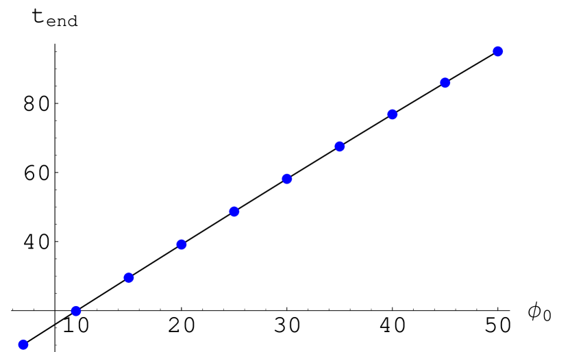
Figure 5: The dependence of $t_{\mathrm{end}}$ on $\phi_{0}$ ($\varepsilon=10^{-5}$, $m=1{.}1$, $S_{20}=10^{-5}$, $S_{20}^{\prime}=0$).

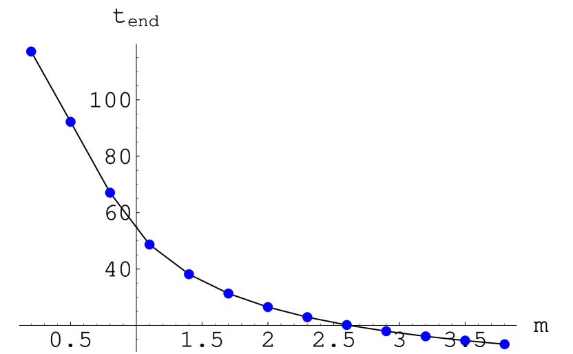
Figure 6: The dependence of $t_{\mathrm{end}}$ on $m$ ($\varepsilon=10^{-5}$, $\phi_{0}=25$, $S_{20}=10^{-5}$, $S_{20}^{\prime}=0$).

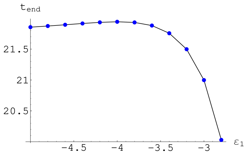
Figure 7: The dependence of $t_{\mathrm{end}}$ on $\varepsilon$ ($\varepsilon=10^{\varepsilon_{1}}$, $\phi_{0}=10$, $m=1{.}0$, $S_{20}=10^{-5}$, $S_{20}^{\prime}=0$).

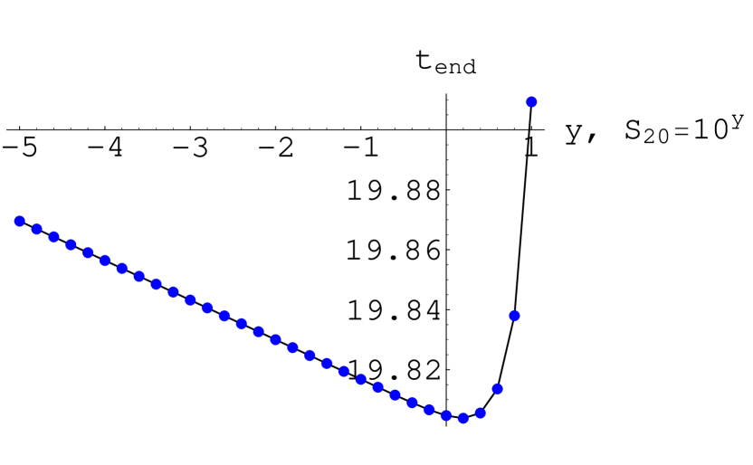
Figure 8: The dependence of $t_{\mathrm{end}}$ on $S_{20}$ ($\varepsilon=10^{-5}$, $m=1.0$, $\phi_{0}=25$, $S_{20}^{\prime}=10^{-4}$).

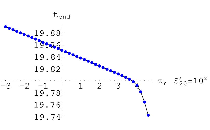
Figure 9: The dependence of $t_{\mathrm{end}}$ on $S_{20}^{\prime}$ ($\varepsilon=10^{-5}$, $\phi_{0}=10$, $m=1.0$, $S_{20}=10^{-5}$).

Similar to GR, the value of duration of inflationary stage depends on initial value of $\phi_{0}$ in linear way (Fig. 5). From numerical analysis of the value of $t_{\mathrm{end}}$ in dependence on parameters and initial conditions follows:

1. similar to GR, there is a lower limit for initial value of $|\phi_{0}|$ to have sufficient number of e-folds during the inflationary stage ($|\phi_{0}|\approx 10$);

2. for given value of $\varepsilon$ admissible values for $|\phi_{0}|$ have upper limit;

3. the parameter $\varepsilon$ has upper limit depending on values $m$, $\phi_{0}$ and $S_{20}^{\prime}$ (in Fig. 7: $\varepsilon\leq 10^{-3}$);

4. there are upper limits for admissible values of $S_{20}$ and $S_{20}^{\prime}$ at given values of $m$, $\varepsilon$ and $\phi_{0}$ (Fig. 8–9).

Note that the presence of relativistic matter besides of scalar field leads only to quantitative corrections and does not change general conclusions given above. In particular, the presence of ultrarelativistic matter at transition stage changes the amplitude of oscillations $S_{2}^{\prime}$-function. The influence of ultrarelativistic matter at inflationary and postinflationary stages is negligibly small because the energy density of ultrarelativistic matter rapidly decreases during inflationary stage.

The behaviour of $H$ and $\phi$ during the inflationary stage are similar to that of GR. (Figures 10). There are small differences for $H$ at the start and the end of inflationary stage. The graphs in Fig. 10 and also in Fig. 11 for $S_{2}$-function are obtained for $m=1.1$, $\varepsilon=10^{-5}$, $\phi_{0}=10$, $S_{20}=0$, $S_{20}^{\prime}=10^{-4}$. During the inflationary stage the following relations are satisfied with a rather high accuracy

$$H\approx\sqrt{\frac{1}{2}m^{2}\phi^{2}+\frac{1}{2}{\phi^{\prime}}^{2}},\qquad S_{2}\approx\sqrt{m^{2}\phi^{2}-\frac{1}{2}{\phi^{\prime}}^{2}}.$$

Figure 10: The behaviour of $H$ (firm line) and $\phi$ (dashed line) during the inflationary stage.

Figure 11: The behaviour of $S_{2}$ during the inflationary stage.

The behaviour of scalar field $\phi$, torsion function $S_{2}$ and Hubble parameter $H$ during the postinflationary stage are presented in Figures 12–14. The graphs in Figures 12, 13 and 14a are obtained at the following values of parameters $\varepsilon=10^{-5}$, $m=1{.}1$ and initial conditions: $\phi_{0}=10$, $S_{20}=0$ and $S_{20}^{\prime}=10^{-4}$. Similar to GR during the postinflationary stage the scalar field $\phi$ oscillates with decreasing amplitude. The frequency of $\phi$-oscillations increases by increasing of the parameter $m$. The oscillations of the Hubble parameter have the character of beats (Fig. 14). Two subsequent pulsation of beats are divided by domain of oscillations with small amplitude. Similar to inflationary models without torsion function $S_{2}$ investigated in [3], for sufficiently large values of the parameter $m$ the oscillating Hubble parameter changes its sign (in Figures 14a and 14b the value of $m$ is equal to 1.1 and 0.4 respectively). In this case the cosmological model vibrates during some time interval after inflation. The amplitude of $H$-beats increases by increasing of parameter $m$. By decreasing of $\varepsilon$ the frequency of oscillation inside one pulsation increases although the frequency of beats oneself practically does not change. There is the correlation between $\phi$-oscillations, $H$-beats and the temporal behaviour of $S_{2}$-function during the postinflationary stage. When instantaneous value of $\phi$ is small in absolute value, then $S_{2}$-function oscillates near zero and $H$ decreases being between two subsequent pulsations. When absolute value of $\phi$ is near to its maximum, the $H$-parameter oscillates inside of pulsation and the absolute value of $S_{2}$-function increases.

Figure 12: The behaviour of $\phi$ during the postinflationary stage.

Figure 13: The behaviour of $S_{2}$ during the postinflationary stage.

Figure 14: The behaviour of $H$ during the postinflationary stage.

As result of this Section, we can conclude that physically interesting solutions exist for some restrictions on parameters $m$, $\varepsilon$ and for sufficiently large domain of initial conditions.

4 Extremum surface for initial conditions

It is interesting to investigate more particularly the structure of extremum surface defined by (13), on which initial conditions for regular inflationary cosmological solutions are given. Supposing below $\rho=0$ and $k=0$, we will have extremum surface in 4-dimensional space of variables ($\phi_{0}$, $\phi_{0}^{\prime}$, $S_{20}$, $S_{20}^{\prime}$). By taking into account results concerning the duration of time $t_{\mathrm{end}}$ obtained in previous Section, we will consider 3-dimensional subspace $P_{3}$ of variables ($S_{20}$, $S_{20}^{\prime}$, $\phi_{0}^{\prime}$), then the relation (13) determines 2-dimensional surface $P_{2}$ in $P_{3}$ depending parametrically on variable $\phi_{0}$ and also on parameters $m$ and $\varepsilon$. The 2-dimensional surface $P_{2}$ has sufficiently complicated structure and includes a closed cover $P_{20}$ and also some complicated surfaces surrounding the closed cover $P_{20}$. A part of surface $P_{2}$ is presented in Figure 15.

As numerical analysis shows, we obtain regular inflationary cosmological solutions by choosing initial conditions on closed cover $P_{20}$. The study of geometrical properties of surface $P_{2}$ allows to understand some important properties of regular inflationary cosmological solutions at transition stage from compression to expansion. With this purpose we will consider cross-sections of the surface $P_{2}$ with planes orthogonal to coordinate axes $S_{20}$, $S_{20}^{\prime}$ and $\phi_{0}^{\prime}$. As example, in Fig. 16 corresponding cross-section in the plane $S_{20}^{\prime}=10^{-4}$ is presented ($m=1{.}1$, $\varepsilon=10^{-5}$, $\phi_{0}=10$).

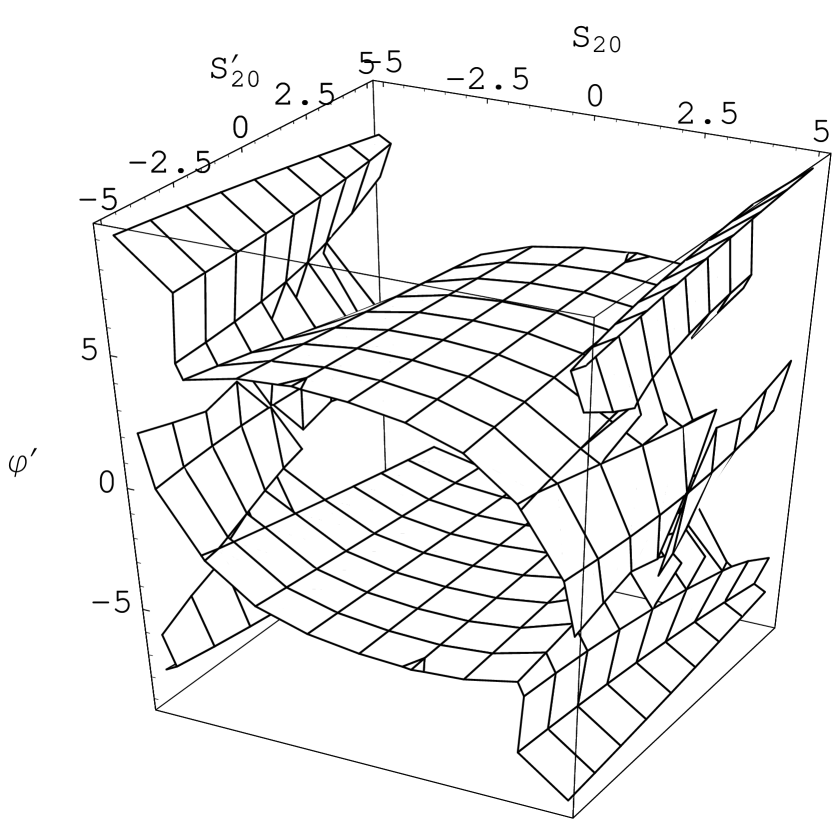
Figure 15: Part of extremum surface $P_{20}$.

Figure 16: Cross-section of extremum surface $P_{20}$ by the plane $S_{20}^{\prime}=10^{-4}$.

By increasing of $m$ and the value of variable $\phi_{0}$ linear sizes of the closed cover $P_{20}$ increase. By decreasing of $\varepsilon$ linear sizes of $P_{20}$ increase only in directions of axes $S_{20}$ and $S_{20}^{\prime}$ and do not change practically in direction of $\phi_{0}^{\prime}$.

As it was discussed in previous Section, the Hubble parameter oscillates at transition stage from compression to expansion. This means that during this stage the quantities $H$, $S_{2}$, $S_{2}^{\prime}$, $\phi$, $\phi^{\prime}$ are changing by intersecting the extremum surface $H=0$ and by changing the sign of derivative $H^{\prime}$. In order to find domains on closed cover $P_{20}$, where the sign of $H^{\prime}$ is positive and negative, we have to consider the intersection of $P_{20}$ with surface $H^{\prime}=0$ defined by (12). The sign of $H^{\prime}$ on $P_{20}$ is different from different sides of intersection line. The place of intersection of $P_{20}$ with surface $H^{\prime}=0$ depends on the value of $\phi_{0}$. So, in the case $\phi_{0}=10$ the domain of intersection corresponds to small values of $S_{20}^{\prime}$ and to values of $S_{20}$ near to its maximum. By increasing of $\phi_{0}$ the domain of intersection moves in direction of decreasing values of $S_{20}$ and increasing values of $S_{20}^{\prime}$. The presence of domains with positive and negative values of derivative $H^{\prime}$ on extremum surface $P_{20}$ allows to explain the oscillating character of the Hubble parameter at transition stage, that is connected essentially with behaviour of $S_{2}$-function (see Fig. 3). After the bounce at $t=0$ the $S_{2}$-function quickly increases and reaches its maximum. As a result, oscillating function $H(t)$ reaches now extremum surface at value of $S_{20}$, where the derivative $H_{0}^{\prime}$ is negative. Together with changing of $S_{2}$-function the process of oscillations of the Hubble parameter is repeated at decreasing values of $\phi_{0}$ (see Fig. 2) and as result at decreasing values of $S_{20\mathrm{max}}$. Oscillations of $H$-function will continue even after this function does not reach extremum surface. The amplitude of $H$-oscillations will continue to decrease until the inflationary stage will come.

5 Conclusion

As follows from our analysis, regular inflationary cosmological solutions for HIM with two torsion functions built in the framework of PGTG are realized at certain restrictions on parameters of HIM and at large domain of initial conditions on extremum surface $H=0$. The presence of pseudoscalar torsion function $S_{2}(t)$ leads to essential changes of considered solutions in comparison with inflationary cosmological solutions for HIM without $S_{2}$-function analyzed in [3]. At first of all these changes relate to properties of transition stage from compression to expansion and post-inflationary stage and are connected with oscillating behaviour of the Hubble parameter. Differences of post-inflationary stages for cosmological solutions in considered theory in comparison with general relativity theory can lead to quantitative differences by transition to radiation-dominated stage, in particular, to differences in anisotropy of relic radiation. This means that the building of perturbation theory for scalar fields in considered inflationary cosmological HIM is of direct physical interest.

References

• [1] Minkevich A V 2006 Gravitation&Cosmology 12 11–21 (Preprint gr-qc/0506140)
• [2] Minkevich A V 2007 Acta Physica Polonica B 38 61–72 (Preprint gr-qc/0512123)
• [3] Minkevich A V and Garkun A S 2006 Class. Quantum Grav. 23 4237–47 (Preprint gr-qc/0512130)
• [4] Minkevich A V, Garkun A S and Kudin V I 2007 Class. Quantum Grav. 24 5835–47 (Preprint Arxiv:0706.1157)
• [5] Minkevich A V 2007 Ann. Fond. Louis de Broglie 32 253–266 (Preprint Arxiv:0709.4337)