Avoiding entanglement sudden-death via measurement feedback control in a quantum network

Abstract

In this paper, we consider a linear quantum network composed of two distantly separated cavities that are connected via a one-way optical field. When one of the cavity is damped and the other is undamped, the overall cavity state obtains a large amount of entanglement in its quadratures. This entanglement however immediately decays and vanishes in a finite time. That is, entanglement sudden-death occurs. We show that the direct measurement feedback method proposed by Wiseman can avoid this entanglement sudden-death, and further, enhance the entanglement. It is also shown that the entangled state under feedback control is robust against signal loss in a realistic detector, indicating the reliability of the proposed direct feedback method in practical situations.

I Introduction

Reliable generation and distribution of entanglement in a quantum network is a central subject in quantum information technology nielsen , especially in quantum communication Cirac ; vanEnk ; Parkins1 ; Parkins2 . The biggest issue in such systems is the decay of entanglement due to decoherence effects that are inevitably introduced when node-channel or channel-environment interaction occurs. Entanglement distillation Bennett1 ; Bennett2 is a useful technique that restores such degraded entanglement. However, it sometimes happens that entanglement completely disappears in a finite time, which is called entanglement sudden-death Eberly1 ; Eberly2 . In this case, distillation techniques cannot recover the vanished entanglement.

On the other hand, feedback control can be used to modify the dynamical structure of a system and improve its performance, e.g., see Doherty1 ; Thomsen ; Ahn ; Bouten . Entanglement protection or generation is one of the most attractive applications of feedback Wang ; Carvalho ; Mirrahimi ; Yamamoto . In particular, two studies have demonstrated that a feedback controller effectively assists in the distribution of entanglement in a quantum network. One such result is by Mancini and Wiseman Mancini , where a direct measurement feedback method Wiseman1 ; Wiseman2 is used to enhance the correlation of two bosonic modes that couple through a $\chi^{(2)}$ nonlinearity. The other such result is by Yanagisawa Yanagisawa , where an estimation-based feedback controller is used to deterministically generate an entangled photon number state of two distantly separated cavities.

This paper follows a similar direction to Mancini and Yanagisawa . That is, we also consider a problem of distributing entanglement in a quantum network using direct feedback control. The quantum network being considered is depicted in Fig. 1: Two spatially separated cavities are connected via a one-way optical field, and the measurement results of the output of Cavity 2 are directly fed back to control both cavities. A more specific description will be given in Sections II-B and II-C, but here we note that the network model considered brings together the following three features that have been not simultaneously considered in previous work. First, the network contains models of realistic components; a realistic quantum channel in contact with an environment and a realistic homodyne detector with finite bandwidth Warszawski1 ; Warszawski2 ; Warszawski3 . A realistic model is of practical importance for real-time quantum feedback control. Second, we consider linear continuous-variable cavity models (i.e., we consider the quadratures of the cavity mode), similar to the case of Parkins1 ; Parkins2 ; Mancini . Hence, the system differs from a discrete-variable system such as an atomic energy level Cirac ; vanEnk , or a photon number system description Yanagisawa . This setup is motivated by the recent rapid progress and deep understanding of continuous-variable systems in the quantum information regime Braunstein . Third, the cavities are spatially separated, and the interaction between them is simply mediated by an optical field, while in Mancini two bosonic modes interact through a $\chi^{(2)}$ optical nonlinearity and thus the two modes are not spatially separated. The spatially separated case is the case of interest in applications such as quantum communication.

Figure 1: Schematic of the network. Thick gray lines represent quantum optical fields, while thin black lines represent classical signals.

The contributions of this paper are as follows. First, we show that the network considered in this paper, which looks complicated, can be systematically captured and described using the theory of quantum cascade systems Carmichael1 ; Carmichael2 ; Gardiner ; Gough . We then show that when the first cavity is undamped and the second cavity is damped, the cavity state obtains a large amount of entanglement, which, however, disappears in a finite time despite the continuous interaction between the cavities; i.e., entanglement sudden-death occurs. As mentioned above, no distillation technique can recover such a zero entanglement. Nevertheless, we show that direct feedback control not only prevents entanglement sudden-death, but can also enhance the entanglement. Moreover, it will be shown that the entangled state under control is robust against signal loss in a realistic detector, implying the reliability of the direct feedback method in practical situations.

We use the following notation. For a matrix $A=(a_{ij})$, the symbols $A^{{\mathsf{T}}}$, $A^{\dagger}$, and $A^{*}$ represent its transpose, conjugate transpose, and elementwise complex conjugate of $A$, i.e., $A^{{\mathsf{T}}}=(a_{ji})$, $A^{\dagger}=(a_{ji}^{*})$, and $A^{*}=(a_{ij}^{*})=(A^{\dagger})^{{\mathsf{T}}}$, respectively. These rules are applied to any rectangular matrix including column and row vectors. ${\rm Re}(A)$ and ${\rm Im}(A)$ denote the real and imaginary part of $A$, respectively, i.e., $({\rm Re}(A))_{ij}=(a_{ij}+a_{ij}^{*})/2$ and $({\rm Im}(A))_{ij}=(a_{ij}-a_{ij}^{*})/2{\rm i}$. The matrix element $a_{ij}$ can be an operator $\hat{a}_{ij}$; in this case, $\hat{a}_{ij}^{*}$ denotes its adjoint operator.

II Model

II.1 General linear quantum systems

We consider a general linear continuous-variable system with $N$-degrees of freedoms. Let $\hat{{\bf x}}_{i}=(\hat{q}_{i},\hat{p}_{i})^{{\mathsf{T}}}$ be the standard quadrature pair of the $i$-th subsystem. It then follows from the canonical commutation relation $[\hat{q}_{i},\hat{p}_{j}]=\hat{q}_{i}\hat{p}_{j}-\hat{p}_{j}\hat{q}_{i}={\rm i}\delta_{ij}~{}(\hbar=1)$ that the vector of system variables $\hat{{\bf x}}:=(\hat{{\bf x}}_{1}^{{\mathsf{T}}},\ldots,\hat{{\bf x}}_{N}^{{\mathsf{T}}})^{{\mathsf{T}}}$ satisfies

$$\hat{{\bf x}}\hat{{\bf x}}^{{\mathsf{T}}}-(\hat{{\bf x}}\hat{{\bf x}}^{{\mathsf{T}}})^{{\mathsf{T}}}={\rm i}\Sigma_{N}={\rm i}\bigoplus_{k=1}^{N}\Sigma,~{}~{}~{}\Sigma:=\left[\begin{array}[]{cc}0&1\\ -1&0\\ \end{array}\right].$$

Suppose that the system contacts with $M$ optical vacuum fields without scattering. In general, such an interaction is described by a unitary operator that obeys the Hudson-Parthasarathy equation Hudson :

$$d\hat{U}_{t}=\Big{[}\big{(}-{\rm i}\hat{H}-\frac{1}{2}\sum_{k=1}^{M}\hat{L}_{k}^{*}\hat{L}_{k}\big{)}dt$$

$$\hskip 15.00002pt\mbox{}+\sum_{k=1}^{M}\big{(}\hat{L}_{k}d\hat{B}_{k,t}^{*}-\hat{L}_{k}^{*}d\hat{B}_{k,t}\big{)}\Big{]}\hat{U}_{t},~{}~{}~{}\hat{U}_{0}=\hat{I}.$$ (1)

The operators $\hat{B}_{k,t}$ and $\hat{B}_{k,t}^{*}$ represent the quantum annihilation and creation processes on the $k$-th field, respectively. Note that $[d\hat{B}_{i,t},d\hat{B}^{*}_{j,t}]=\delta_{ij}dt$. Let us choose $\hat{H}=\hat{H}^{*}$ and $\hat{L}_{k}$ as follows:

$$\hat{H}=\frac{1}{2}\hat{{\bf x}}^{{\mathsf{T}}}G\hat{{\bf x}},~{}~{}~{}\hat{L}_{k}=L_{k}^{{\mathsf{T}}}\hat{{\bf x}},$$ (2)

where $G=G^{{\mathsf{T}}}\in{\mathbb{R}}^{2N\times 2N}$ and $L_{k}\in{\mathbb{C}}^{2N}$. The system variables obey the Heisenberg equation $\hat{{\bf x}}_{t}:=(\ldots,\hat{U}_{t}^{*}\hat{q}_{i}\hat{U}_{t},\hat{U}_{t}^{*}\hat{p}_{i}\hat{U}_{t},\ldots)^{{\mathsf{T}}}$. We then obtain the following linear equation:

$$d\hat{{\bf x}}_{t}=A\hat{{\bf x}}_{t}dt+{\rm i}\Sigma_{N}[L^{{\mathsf{T}}}d\hat{{\bf B}}_{t}^{*}-L^{\dagger}d\hat{{\bf B}}_{t}],$$ (3)

where $L^{{\mathsf{T}}}:=(L_{1},\ldots,L_{M})\in{\mathbb{C}}^{2N\times M}$, $A:=\Sigma_{N}[G+{\rm Im}(L^{\dagger}L)]$, and $\hat{{\bf B}}_{t}:=(\hat{B}_{1,t},\ldots,\hat{B}_{M,t})^{{\mathsf{T}}}$. For details on the physical meaning of these abstract linear models, see Section III and, e.g., Edwards ; JNP06 ; NJD08 . It is easy to see that the first moment vector $\langle{\hat{{\bf x}}_{t}}\rangle:=(\ldots,\langle{\hat{U}_{t}^{*}\hat{q}_{i}\hat{U}_{t}}\rangle,\langle{\hat{U}_{t}^{*}\hat{p}_{i}\hat{U}_{t}}\rangle,\ldots)^{{\mathsf{T}}}$, where $\langle{\hat{x}}\rangle:={\rm Tr}\hskip 1.9919pt(\hat{\rho}\hat{x})$, satisfies the linear equation $d\langle{\hat{{\bf x}}_{t}}\rangle/dt=A\langle{\hat{{\bf x}}_{t}}\rangle$. Also, the covariance matrix $V_{t}=(\langle{\hat{{\bf V}}_{ij}}\rangle)$, where

$$\hat{{\bf V}}=\frac{1}{2}\Big{[}\Delta\hat{{\bf x}}_{t}\Delta\hat{{\bf x}}_{t}^{{\mathsf{T}}}+(\Delta\hat{{\bf x}}_{t}\Delta\hat{{\bf x}}_{t}^{{\mathsf{T}}})^{{\mathsf{T}}}\Big{]},~{}~{}~{}\Delta\hat{{\bf x}}_{t}:=\hat{{\bf x}}_{t}-\langle{\hat{{\bf x}}_{t}}\rangle,$$

satisfies the following Lyapunov matrix differential equation:

$$\frac{dV_{t}}{dt}=AV_{t}+V_{t}A^{{\mathsf{T}}}+D.$$ (4)

Here, $D:=\Sigma_{N}{\rm Re}(L^{\dagger}L)\Sigma_{N}^{{\mathsf{T}}}$. Suppose that the quantum state is Gaussian at $t=0$. Then, from the linearity of the dynamics, the unconditional state is always Gaussian with mean $\langle{\hat{{\bf x}}_{t}}\rangle$ and covariance $V_{t}$. Note that the unconditional state corresponds to a classical probability density that describes a linear diffusion process.

II.2 The ideal network

Before describing the quantum network depicted in Fig. 1, let us consider the ideal situation where the optical field between the cavities is not in contact with any environment, and the homodyne detector is perfect. In this case, the system is the simple cascade of two cavities with a feedback loop. The entangled state of this ideal network will be compared to that of the realistic one for the purpose of clarifying how much the realistic parameters affect the system. Also, this ideal setup allows us to determine a reasonable control Hamiltonian (the vector $f$ given below), as will be seen in Section III-B.

Each component of the network is described as follows. The optical vacuum field $\hat{B}_{1,t}$ comes into Cavity 1, and then, its output becomes the input of Cavity 2. We assume that, after some approximations, the $i$-th cavity-field interaction is represented by Eq. (II.1) with single field $(M=1)$ and with the following operators:

$$\hat{H}_{i}=\frac{1}{2}\hat{{\bf x}}_{i}^{{\mathsf{T}}}G_{i}\hat{{\bf x}}_{i},~{}~{}~{}\hat{L}_{1,i}=\ell_{i}^{{\mathsf{T}}}\hat{{\bf x}}_{i},~{}~{}~{}(i=1,2),$$

where $\hat{q}_{i}=(\hat{a}_{i}+\hat{a}_{i}^{*})/\sqrt{2}$ and $\hat{p}_{i}=(\hat{a}_{i}-\hat{a}_{i}^{*})/\sqrt{2}{\rm i}$. The subscript $(1,i)$ in $\hat{L}$ means the $1$-st field and the $i$-th cavity (see the figures in Appendix A). Also, $G_{i}=G_{i}^{{\mathsf{T}}}\in{\mathbb{R}}^{2\times 2}$ and $\ell_{i}\in{\mathbb{C}}^{2}$. The output of Cavity 2 is transformed to a classical signal $y_{t}$ through an ideal homodyne detector. Suppose now that each cavity has an additional Hamiltonian of the form

$$\hat{H}_{i}^{\rm fb}=u_{t}\hat{F}_{i}=u_{t}f_{i}^{{\mathsf{T}}}\hat{{\bf x}}_{i},~{}~{}~{}f_{i}\in{\mathbb{R}}^{2},~{}~{}~{}(i=1,2),$$

where $u_{t}\in{\mathbb{R}}$ is the control input. Then, direct measurement feedback $u_{t}=gy_{t}$ closes the loop by connecting the detector to the cavities. Here $g\in{\mathbb{R}}$ is the control gain. Note that we need a classical communication channel in order to control Cavity 1; that is, a local operation via classical communication (LOCC) type control is performed.

For this network, we can easily determine the system matrices $G$ and $L_{k}$ in Eq. (2) that specify the whole dynamical equation. The derivation is based on the theory of quantum cascade systems Carmichael1 ; Carmichael2 ; Gardiner ; Gough and is given in Appendix A. Then, from the definition, the $A$ and $D$ matrices in the Lyapunov equation (4) are readily obtained as follows:

$$A_{\rm id}=A_{o}+2g\Sigma_{2}f{\rm Re}(\ell)^{{\mathsf{T}}},$$ (5)

$$D_{\rm id}=D_{o}+\Sigma_{2}\big{[}g^{2}ff^{{\mathsf{T}}}-g{\rm Im}(\ell)f^{{\mathsf{T}}}-gf{\rm Im}(\ell)^{{\mathsf{T}}}\big{]}\Sigma_{2}^{{\mathsf{T}}},$$ (6)

where $\ell=(\ell_{1}^{{\mathsf{T}}},\ell_{2}^{{\mathsf{T}}})^{{\mathsf{T}}},~{}f=(f_{1}^{{\mathsf{T}}},f_{2}^{{\mathsf{T}}})^{{\mathsf{T}}}$, and

$$A_{o}=\left[\begin{array}[]{cc}A_{1}&0\\ 2\Sigma{\rm Im}(\ell_{2}^{*}\ell_{1}^{{\mathsf{T}}})&A_{2}\\ \end{array}\right],~{}~{}D_{o}=\left[\begin{array}[]{cc}D_{1}&\star\\ \Sigma{\rm Re}(\ell_{2}^{*}\ell_{1}^{{\mathsf{T}}})\Sigma^{{\mathsf{T}}}&D_{2}\\ \end{array}\right].$$ (7)

Here, $A_{i}=\Sigma[G_{i}+{\rm Im}(\ell_{i}^{*}\ell_{i}^{{\mathsf{T}}})]$, $D_{i}=\Sigma{\rm Re}(\ell_{i}^{*}\ell_{i}^{{\mathsf{T}}})\Sigma^{{\mathsf{T}}}$, and $\star$ denotes the symmetric elements. Note that $A_{o}$ and $D_{o}$ are the system matrices of the network without feedback. Hence, the upper off-diagonal block matrix of $A_{o}$ is zero, implying the one-way interaction of the cavities.

II.3 The realistic network

We are now in the position to describe a realistic network, which introduces the following two assumptions. First, the output of Cavity 1 is mixed with another vacuum field $\hat{B}_{2,t}$ through a beam splitter (BS) with transmittance $\alpha$. This is a standard model of possible environmental effects on a long quantum channel. Second, the homodyne detector is not perfect and is described by the one-dimensional classical dynamics

$$d\xi_{t}=a_{1}\xi_{t}dt+a_{2}dw_{t},~{}~{}dy_{t}=a_{3}\xi_{t}dt+dv_{t},~{}~{}a_{i}\in{\mathbb{R}},$$ (8)

where $w_{t}$ is an input stochastic process satisfying ${\bf E}[dw_{t}^{2}]=dt$ and $v_{t}$ is an additional measurement noise satisfying ${\bf E}[dv_{t}^{2}]=a_{4}dt~{}(a_{4}>0)$. In particular, a typical low-pass filter (LPF) is realized by choosing $a_{i}$ as

$$a_{1}=-\frac{1}{\tau},~{}~{}~{}a_{2}=\frac{1}{\tau},~{}~{}~{}a_{3}=1,$$

where $\tau>0$ is the time-constant. We now note that the detector (8) can be represented as a quantum system with two fields $w_{t}=\hat{B}_{1,t}^{{}^{\prime}}+\hat{B}_{1,t}^{{}^{\prime}*}$ and $v_{t}=\hat{B}_{3,t}+\hat{B}_{3,t}^{*}$, where $\hat{B}_{1,t}^{{}^{\prime}}$ is the output of Cavity 2. Indeed, from Gough , Eq. (II.1) with $M=2$ and with the operators

$$\hat{H}_{3}=\frac{a_{1}}{2}(\hat{q}_{3}\hat{p}_{3}+\hat{p}_{3}\hat{q}_{3}),~{}~{}~{}\hat{L}_{1,3}=-{\rm i}a_{2}\hat{p}_{3},~{}~{}~{}\hat{L}_{3,3}=\frac{a_{3}}{2a_{4}}\hat{q}_{3}$$

leads to a linear equation of the form (8), where $\hat{U}_{t}^{*}\hat{q}_{3}\hat{U}_{t}$ plays the same role of $\xi_{t}$.

Consequently, the network is composed of two cavities, a beam splitter, a detector, and a controller, with three optical vacuum fields. (Note that the beam splitter with local oscillator (LO) shown in Fig. 1 is a part of the detector.) To systematically obtain the overall system matrices $G$ and $L_{k}$ in Eq. (2) of this complicated network, we again use the theory of quantum cascade systems Carmichael1 ; Carmichael2 ; Gardiner ; Gough . The procedure is given in Appendix A. We then obtain the matrices $A$ and $D$ in Eq. (4) as follows:

$$A_{\rm re}=\left[\begin{array}[]{ccc}A_{1}&0&ga_{3}\Sigma f_{1}\\ 2\alpha\Sigma{\rm Im}(\ell_{2}^{*}\ell_{1}^{{\mathsf{T}}})&A_{2}&ga_{3}\Sigma f_{2}\\ 2\alpha a_{2}{\rm Re}(\ell_{1})^{{\mathsf{T}}}&2a_{2}{\rm Re}(\ell_{2})^{{\mathsf{T}}}&a_{1}\\ \end{array}\right],$$ (12)

$$D_{\rm re}=\left[\begin{array}[]{ccc}D_{1}&\star&\star\\ \alpha\Sigma{\rm Re}(\ell_{2}^{*}\ell_{1}^{{\mathsf{T}}})\Sigma^{{\mathsf{T}}}&D_{2}&\star\\ -\alpha a_{2}{\rm Im}(\ell_{1})^{{\mathsf{T}}}\Sigma^{{\mathsf{T}}}&-a_{2}{\rm Im}(\ell_{2})^{{\mathsf{T}}}\Sigma^{{\mathsf{T}}}&a_{2}^{2}\\ \end{array}\right]$$ (16)

$$\hskip 20.00003pt\mbox{}+g^{2}a_{4}\left[\begin{array}[]{ccc}\Sigma f_{1}f_{1}^{{\mathsf{T}}}\Sigma^{{\mathsf{T}}}&\star&0\\ \Sigma f_{2}f_{1}^{{\mathsf{T}}}\Sigma^{{\mathsf{T}}}&\Sigma f_{2}f_{2}^{{\mathsf{T}}}\Sigma^{{\mathsf{T}}}&0\\ 0&0&0\\ \end{array}\right].$$ (20)

III Entanglement control

In this section, we study the entanglement of the cavity state for the ideal network. Since the state is Gaussian, its entanglement is completely characterized by the covariance matrix Duan ; Simon . In our case, the covariance matrix to be evaluated is obtained by solving the Lyapunov equation (4) with the coefficient matrices $A_{\rm id}$ and $D_{\rm id}$ in Eqs. (5) and (6). Let the matrices $V_{i}$ be defined by the $2\times 2$ block matrix decomposition of $V$ as follows:

$$V=\left[\begin{array}[]{cc}V_{1}&V_{2}\\ V_{2}^{{\mathsf{T}}}&V_{3}\\ \end{array}\right].$$

Then, the following logarithmic negativity Vidal can be used as a reasonable measure of Gaussian entanglement:

$$E_{\cal N}={\rm max}\big{\{}0,~{}-\log(2\nu)\big{\}},$$ (21)

where $\log x$ denotes the natural logarithm of $x$,

$$\nu:=\frac{1}{\sqrt{2}}\sqrt{\tilde{\Delta}-\sqrt{\tilde{\Delta}^{2}-4{\rm det}(V)}},$$ (22)

$$\tilde{\Delta}:={\rm det}(V_{1})+{\rm det}(V_{3})-2{\rm det}(V_{2}).$$

The logarithmic negativity $E_{\cal N}$ divides the state space into two regions: (i) the separable region, corresponding to $E_{\cal N}=0$, and (ii) the entangled region, within which $E_{\cal N}>0$. Thus phenomena of entanglement creation and destruction can be understood simply in terms of movement of the system between these two regions.

III.1 Entanglement sudden-death

Here we study the uncontrolled network; i.e., $g=0$.

We compute $E_{\cal N}$ for two situations. First, consider the case where both cavities have the same quadratic Hamiltonian and are damped as a result of the field-cavity interaction, that is,

$$G_{1}=G_{2}=\left[\begin{array}[]{cc}m&0\\ 0&1\\ \end{array}\right],~{}~{}~{}\ell_{1}=\ell_{2}=\sqrt{\kappa}\left[\begin{array}[]{c}1\\ {\rm i}\\ \end{array}\right],$$

where $m>0$ and $\kappa>0$. This type of quadratic Hamiltonian can be implemented in a cavity system following the scheme of the degenerate parametric amplification Gardiner ; see Appendix B. In this case, $A_{{\rm id}}$ is a stable matrix, and the Lyapunov equation (4) has a unique steady state solution (see e.g., Zhou ). Now assume that at $t=0$, the cavity is in the separable state satisfying $V_{0}=2I$. When the optical field is switched on, the cavity modes couple after a finite time (i.e., the “entanglement sudden-birth” Ficek occurs), and a steady entangled state is generated as seen from the dotted line in Fig. 2 (a). However, in this case, the entanglement is very small ($E_{\cal N}\approx 0.21$).

This result can be understood by examining the trajectory of the parameter $(\tilde{\Delta},{\rm det}(V))$. In Fig. 3, the colored region with contour lines represents the set of parameters where a general two-mode Gaussian state is entangled, i.e., $E_{\cal N}>0$, while the white region corresponds to separable states; i.e., $E_{\cal N}=0$. The trajectory, denoted by ${\cal T}_{\rm dam}$, evolves toward the steady entangled state that is located far from the area with large $E_{\cal N}$ (the right bottom area in Fig. 3). This is likely because each cavity has a strong tendency to transit into the vacuum state due to the damping. Indeed, when the cavity is in the separable vacuum state $|{0}\rangle|{0}\rangle$, the corresponding covariance matrix satisfies $(\tilde{\Delta},{\rm det}(V))=(0.5,0.0625)$, which is very close to the equilibrium point of ${\cal T}_{\rm dam}$. Moreover, Fig. 2 (b) shows that the purity (for a discussion of physical meanings of the purity, see e.g. Paris ) of the steady Gaussian state $\hat{\rho}$,

$$P:={\rm Tr}\hskip 1.9919pt(\hat{\rho}^{2})=\frac{1}{4\sqrt{{\rm det}(V)}}\in(0,1],$$ (23)

approaches $P\approx 0.8$ as $t\rightarrow\infty$. This also suggests that the steady state is close to the separable vacuum state.

The above observation motivates us to try a dispersive field-cavity interaction, which results in a phase shift of the output field Doherty1 ; Milburn ; Doherty2 ; Wiseman4 . For a practical method to implement this kind of coupling in a cavity system, see Appendix B. In this case, the cavity is not damped, and thus, it does not have a tendency to move toward the vacuum state. In particular, we assume that only the first cavity has such an interaction; i.e.,

$$\ell_{1}=(\sqrt{\kappa},~{}0)^{{\mathsf{T}}},~{}~{}~{}\ell_{2}=\sqrt{\kappa}(1,~{}{\rm i})^{{\mathsf{T}}}.$$

We then find that $A_{\rm id}$ is not a stable matrix, and the Lyapunov equation (4) need not have a steady state solution as $t\rightarrow\infty$ . Fig. 3 shows that the corresponding trajectory, denoted by ${\cal T}_{\rm dis}$, evolves far from the separable initial state and reaches the area with large $E_{\cal N}$. This figure also shows how both the entanglement and purity decreases as time goes on and ${\cal T}_{\rm dis}$ escapes from the region of entangled states at $t=6.2$.

Finally, we remark that, if we exchange the order of the interactions, i.e., $\ell_{1}=\sqrt{\kappa}(1,~{}{\rm i})^{{\mathsf{T}}}$ and $\ell_{2}=(\sqrt{\kappa},~{}0)^{{\mathsf{T}}}$, the corresponding trajectory remains within the region of separable states, i.e., $E_{\cal N}=0$ for all $t>0$. The situation is much the same even when each cavity interacts with the field in a dispersive way.

Figure 2: Time-dependence of the logarithmic negativity (a) and the purity (b) of the overall cavity state without feedback control. The solid and dotted lines correspond to the dispersive-damped and damped-damped cases, respectively. The parameters are $m=0.2$ and $\kappa=1$.

Figure 3: Trajectories of the parameter $(\tilde{\Delta},{\rm det}(V))$ without feedback control. ${\cal T}_{\rm dam}$ and ${\cal T}_{\rm dis}$ correspond to the damped-damped and dispersive-damped cases, respectively. We set $V_{0}=2I$ at $t=0$, from which $\tilde{\Delta}=8$ and ${\rm det}(V_{0})=16$ follow. ($\tilde{\Delta}$ and ${\rm det}(V)$ are in units of $\hbar=1$ and $\hbar^{2}=1$, respectively.)

III.2 Feedback control

We first discuss how to determine the coefficient vector $f=(f_{1}^{{\mathsf{T}}},f_{2}^{{\mathsf{T}}})^{{\mathsf{T}}}$ that realizes high-quality entanglement control. Fortunately, in the ideal case, we can explicitly find such an $f$. The idea was originally provided by Wiseman and Doherty in Wiseman3 , but here we apply the idea in a slightly different manner.

Assume that $g=1$. Then, the Lyapunov equation (4) with coefficient matrices $A_{\rm id}$ and $D_{\rm id}$ in Eqs. (5) and (6) can be rewritten as

$$\frac{dV_{t}}{dt}={\cal R}(V_{t})+\Sigma_{2}(f-f_{t})(f-f_{t})^{{\mathsf{T}}}\Sigma_{2}^{{\mathsf{T}}},$$ (24)

where

$$f_{t}:=2\Sigma_{2}V_{t}{\rm Re}(\ell)+{\rm Im}(\ell)$$ (25)

and

$${\cal R}(V):=A_{o}V+VA_{o}^{{\mathsf{T}}}+D_{o}$$

$$\hskip 20.00003pt\mbox{}-\Big{[}2V{\rm Re}(\ell)-\Sigma_{2}{\rm Im}(\ell)\Big{]}\Big{[}2V{\rm Re}(\ell)-\Sigma_{2}{\rm Im}(\ell)\Big{]}^{{\mathsf{T}}}.$$

We now recall from Fig. 2 (b) that entanglement sudden-death occurs simultaneously with a decrease of the purity (23). This suggests that preventing a decrease of purity may also prevent entanglement sudden-death. However, we should point out that it is not apparent that this will always be the case and the relationship between loss of purity and entanglement sudden-death needs to be studied further. Therefore, a simple control strategy that we try here is to find a feedback controller that prevents an increase of ${\rm det}(V_{t})$ in order to keep the purity high. As the second term of the right-hand side of Eq. (24) is always non-negative, it is then reasonable to choose the time-variant coefficient vector $f=f_{t}$. Of course, this intuitive argument does not always allow us to conclude that ${\rm det}(V_{t})$ takes its minimum value. However, it is known that the algebraic Riccati equation ${\cal R}(V)=0$ has a solution satisfying ${\rm det}(V)=1/16$, which implies that the maximum purity $P=1$ is achieved; e.g., see Wiseman3 . Now assume that Eq. (24) has a unique steady solution $V_{\infty}$ for a constant $f$. Then, by taking the time-invariant coefficient vector

$$\bar{f}:=2\Sigma_{2}V_{\infty}{\rm Re}(\ell)+{\rm Im}(\ell),~{}~{}~{}{\cal R}(V_{\infty})=0,$$ (26)

we obtain the same desirable result, ${\rm det}(V_{\infty})=1/16$. Note that the numerical solution to the algebraic Riccati equation ${\cal R}(V_{\infty})=0$ can readily be obtained using a standard software package such as matlab.

We now consider direct feedback control with the coefficient vector (26). Let us begin with the case where the first cavity-field interaction occurs dispersively. For this system, it is expected from Fig. 3 that the trajectory ${\cal T}_{\rm dis}$ can be modified and stabilized via feedback so that it has an equilibrium point in the area where $E_{\cal N}$ is large. That this is indeed true is shown below. When the parameters are given by $m=0.2$ and $\kappa=1$, we find that $\bar{f}=(0.1212,2.2196,-0.3163,-3.2277)^{{\mathsf{T}}}$ from (26). Fig. 5 illustrates that the controlled trajectory, denoted by ${\cal T}_{\rm dis}^{\rm c}$, indeed shows the convergence that we had hoped for. The entanglement and the purity of the steady cavity state are shown in Fig. 4. While $\bar{f}$ is determined with fixed $g=1$, we consider variations in $g$ to gain understanding about its effect on the control system. When control is not used ($g=0$), the pair of dispersive and damped cavities does not settle down to a steady state as seen in Section III-A, and we find that $E_{\cal N}\rightarrow 0$ as $t\rightarrow\infty$. On the other hand, even with the small-gain feedback controller, the system becomes stable and has a unique steady state with nonzero entanglement. Remarkably, when $g=1$, the entanglement of the steady state ($E_{\cal N}\approx 2.2$) improves upon the maximum value of $E_{\cal N}$ of the uncontrolled state ($E_{\cal N}\approx 0.65$) shown in Fig. 2 (a). Hence we see that direct feedback not only prevents entanglement sudden-death, but can also enhance the entanglement.

Feedback can also improve the entanglement of a system where both cavities are damped, but it is still very small as seen from the dotted line in Fig. 4 (a). (The coefficient vector defined by Eq. (26) in this case is calculated to be $\bar{f}=(0.0629,0.1525,0.2479,-0.5830)$.) To understand this phenomenon, we recall that the uncontrolled trajectory ${\cal T}_{\rm dam}$ has an equilibrium point that is located far from the area with large $E_{\cal N}$. Hence, it should be hard to drastically modify this trajectory such that it could reach that area. It is actually observed in Fig. 5 that, even with the vector $\bar{f}$, the controlled trajectory ${\cal T}_{\rm dam}^{\rm c}$ shows almost the same time-evolution as the autonomous one ${\cal T}_{\rm dam}$.

The above results suggest that strong stability of the autonomous system sometimes makes it difficult for the state to transit into a desirable entangled target.

Figure 4: The logarithmic negativity (a) and the purity (b) of the steady cavity state with feedback control. $g$ is the control gain. The solid and dotted lines correspond to the dispersive-damped and damped-damped cases, respectively. The parameters are $m=0.2$ and $\kappa=1$.

Figure 5: Trajectories of the parameters $(\tilde{\Delta},{\rm det}(V))$ with feedback control. ${\cal T}_{\rm dam}^{\rm c}$ and ${\cal T}_{\rm dis}^{\rm c}$ correspond to the damped-damped and dispersive-damped cases, respectively. The initial state is the same as before: $V_{0}=2I$.

IV A realistic control scenario

Finally, we return to the original setup of the network. That is, the quantum channel is in contact with an environment, and the homodyne detector is replaced by a realistic LPF with finite bandwidth. The purpose here is to study the impacts of these realistic components on the entanglement of the cavity state. The covariance matrix of the cavity state corresponds to the left-upper $4\times 4$ submatrix of $V_{t}$ that is the solution of Eq. (4) with $A_{\rm re}$ and $D_{\rm re}$ given in Eqs. (12) and (16). Note that the cavity state is the reduced one with the detector mode traced out. We here focus only on the network where the first cavity interacts with the field dispersively. For the control Hamiltonian, we use the same coefficient vector $\bar{f}=(0.1212,2.2196,-0.3163,-3.2277)^{{\mathsf{T}}}$. It should be noted that, in this realistic case, we cannot follow the discussion in Section III-B to obtain a reasonable coefficient vector $f$.

First, consider Fig. 6 (a). This shows some plots of $E_{\cal N}$ with the time-constant $\tau$ changing between $0.01\leq\tau\leq 0.6$ and with the fixed transmittance $\alpha=1$ (i.e., no loss in the channel). The most upper line almost coincides with the ideal one shown in Fig. 4 (a). That is, the entanglement in the realistic situation continuously converges to the ideal one as $\tau\rightarrow 0$. We also observe that the degradation of $E_{\cal N}$ is small with respect to $\tau$. Since the detector is regarded as a component of the controller, these results imply that the realistic direct feedback is robust against signal loss in the LPF. In other words, direct feedback control is reliable even in this realistic situation.

On the other hand, Fig. 6 (b) plots $E_{\cal N}$ for some values of the channel loss $\beta:=1-\alpha$ with fixed $\tau=0.01$. We find that $E_{\cal N}$ converges to the ideal one as $\beta\rightarrow 0$, similar to the above case. However, in this case, $E_{\cal N}$ rapidly decreases with respect to $\beta$. Even for the very small loss $\beta=0.01$, a visible degradation occurs. Moreover, when $\beta=0.1$, which still means we have a high-quality quantum channel, $E_{\cal N}$ decreases less than half of the ideal one. That is, the entanglement is fragile to realistic channel loss.

The above results are reasonable because the channel loss directly reflects the decrease of interaction strength, while the finite bandwidth of LPF simply implies loss of a classical signal. Hence the former should be a critical factor for entanglement generation.

Figure 6: The logarithmic negativity of the steady cavity state with feedback control. $g$ is the control gain. (a) From the top downwards, the lines correspond to $\tau=0.01,0.2,0.4,0.6$, while $\alpha=1$. (b) From the top downwards, the lines correspond to $\alpha=1,0.99,0.95,0.90$, while $\tau=0.01$. In both cases, the LPF noise is very small; $a_{4}=0.01$. The parameters are $m=0.2$ and $\kappa=1$.

V Conclusion

The contributions of this paper are summarized as follows. First, it was shown that, when the first cavity is undamped and the second one is damped, the overall cavity state obtains a significant amount of entanglement, which however disappears in a finite time. Then, we have shown that direct measurement feedback can avoid this entanglement sudden-death, and further, enhances the entanglement. Moreover, it was shown that the direct feedback controller is reliable under the influence of signal loss in a realistic detector, although imperfection in the quantum channel is a critical issue that largely degrades the achieved entanglement. We believe that the case study we have presented provides useful insights that may be of use for more complex quantum network engineering.

Appendix A Quantum cascade systems

A.1 General theory

In this appendix, we begin with a review of the theory of quantum cascade systems which was originally developed by Carmichael Carmichael1 ; Carmichael2 and Gardiner Gardiner in a quantum optics framework and recently reformulated in more general setting by Gough and James Gough . We then apply the theory to our model and derive the corresponding system matrices.

The most general form of quantum dynamics that interacts with $M$ optical input fields is described by the following unitary evolution:

$$d\hat{U}_{t}=\Big{[}\big{(}-{\rm i}\hat{H}-\frac{1}{2}\sum_{k=1}^{M}\hat{L}_{k}^{*}\hat{L}_{k}\big{)}dt$$

$$\hskip 15.00002pt\mbox{}+\sum_{k=1}^{M}\hat{L}_{k}d\hat{B}_{k,t}^{*}-\sum_{k,j=1}^{M}\hat{L}_{j}^{*}\hat{S}_{jk}d\hat{B}_{j,t}$$

$$\hskip 15.00002pt\mbox{}+\sum_{k,j=1}^{M}(\hat{S}_{kj}-\delta_{kj})d\hat{\Lambda}_{kj}\Big{]}\hat{U}_{t},~{}~{}~{}\hat{U}_{0}=\hat{I}.$$ (27)

This is also called the Hudson-Parthasarathy equation Hudson . Here, the operators $\hat{B}_{k,t}$ and $\hat{B}_{k,t}^{*}$ represent the quantum annihilation and creation processes on the $k$-th field, respectively. The operator $\hat{\Lambda}_{kj}$ represents the scattering process from the $k$-th state to the $j$-th state, and it satisfies $d\hat{\Lambda}_{ij}d\hat{\Lambda}_{kl}=\delta_{jk}d\hat{\Lambda}_{il}$. The matrix of operators $\hat{{\bf S}}:=(\hat{S}_{ij})$ must satisfy $\hat{{\bf S}}^{\dagger}\hat{{\bf S}}=\hat{{\bf S}}\hat{{\bf S}}^{\dagger}=I$ in order for $\hat{U}_{t}$ to be unitary. The system is completely characterized by the triple ${\bf\Gamma}=(\hat{{\bf S}},\hat{{\bf L}},\hat{H})$, where $\hat{{\bf L}}$ is a vector of operators $\hat{{\bf L}}:=(\hat{L}_{1},\ldots,\hat{L}_{M})^{{\mathsf{T}}}$. Let $\hat{X}$ be an operator of the system. Then, this evolves in time according to the Heisenberg equation $\hat{X}\rightarrow j_{t}(\hat{X}):=\hat{U}_{t}^{*}\hat{X}\hat{U}_{t}$. In particular, we can define $M$ output fields $\hat{B}^{\prime}_{k,t}:=j_{t}(\hat{B}_{k,t})$, which yields

$$d\hat{{\bf B}}^{\prime}_{t}=j_{t}(\hat{{\bf L}})dt+j_{t}(\hat{{\bf S}})d\hat{{\bf B}}_{t},$$

where we have defined $\hat{{\bf B}}^{\prime}_{t}:=(\hat{B}^{\prime}_{1,t},\ldots,\hat{B}^{\prime}_{M,t})^{{\mathsf{T}}},j_{t}(\hat{{\bf L}}):=(j_{t}(\hat{L}_{1}),\ldots,j_{t}(\hat{L}_{M}))^{{\mathsf{T}}}$, etc.

Let us now consider two systems: ${\bf\Gamma}_{1}=(\hat{{\bf S}}_{1},\hat{{\bf L}}_{1},\hat{H}_{1})$ and ${\bf\Gamma}_{2}=(\hat{{\bf S}}_{2},\hat{{\bf L}}_{2},\hat{H}_{2})$. Note that the number of inputs (i.e., outputs) of these systems can always be matched by introducing additional components $0$ in $\hat{{\bf L}}$ and $I$ in $\hat{{\bf S}}$ as $\hat{{\bf L}}\oplus 0$ and $\hat{{\bf S}}\oplus I$. These systems can be connected so that the outputs of ${\bf\Gamma}_{1}$ are the inputs of ${\bf\Gamma}_{2}$, as depicted abstractly in Fig. 7. We denote this cascade system by ${\bf\Gamma}_{2}\vartriangleleft{\bf\Gamma}_{1}$.

Figure 7: Abstract illustration of the cascade system. The black circles represent that the subsystem interacts with the field.

Then, from Gough , we have

$${\bf\Gamma}_{2}\vartriangleleft{\bf\Gamma}_{1}=\Big{(}\hat{{\bf S}}_{2}\hat{{\bf S}}_{1},~{}\hat{{\bf L}}_{2}+\hat{{\bf S}}_{2}\hat{{\bf L}}_{1},~{}$$

$$\hskip 15.00002pt\hat{H}_{1}+\hat{H}_{2}+\frac{1}{2{\rm i}}(\hat{{\bf L}}_{2}^{\dagger}\hat{{\bf S}}_{2}\hat{{\bf L}}_{1}-\hat{{\bf L}}_{1}^{\dagger}\hat{{\bf S}}_{2}^{\dagger}\hat{{\bf L}}_{2})\Big{)},$$ (28)

where $\hat{{\bf L}}_{k}^{\dagger}=(\hat{L}_{1,k}^{*},\ldots,\hat{L}_{M,k}^{*}),~{}(k=1,2)$ and $\hat{{\bf S}}^{\dagger}=(\hat{S}_{ji}^{*})$.

Direct measurement feedback Wiseman1 ; Wiseman2 is no more than a cascade of the system and the controller. Hence, the overall system representation of the controlled network is readily derived using Eq. (A.1) as follows. For simplicity, let us consider a single-input single-output system ${\bf\Gamma}=(\hat{S},\hat{L},\hat{H}+u_{t}\hat{F})$, where $u_{t}$ represents the control input. An ideal homodyne detector yields a classical signal $y_{t}=j_{t}(\hat{B}_{t}+\hat{B}_{t}^{*})$. Then, the direct feedback $u_{t}=gy_{t}$ closes the loop and realizes

$${\bf\Gamma}_{\rm fb}=(1,-{\rm i}g\hat{F},0)\vartriangleleft(\hat{S},\hat{L},\hat{H})$$

$$\hskip 6.99997pt=\Big{(}\hat{S},~{}\hat{L}-{\rm i}g\hat{F},~{}\hat{H}+\frac{g}{2}(\hat{F}\hat{L}+\hat{L}^{*}\hat{F})\Big{)}.$$ (29)

For a more detailed discussion, see Gough .

A.2 Ideal network

Let us then apply the above formulas to our system. First, we consider an ideal network composed of the following three subsystems:

$$\mbox{Cavity 1:}~{}~{}{\bf C}_{1}=(I,~{}\hat{L}_{1,1},~{}\hat{H}_{1}),$$

$$\mbox{Cavity 2:}~{}~{}{\bf C}_{2}=(I,~{}\hat{L}_{1,2},~{}\hat{H}_{2}),$$

$$\mbox{Controller:}~{}~{}{\bf F}=(I,\hskip 3.00003pt-{\rm i}g\hat{F},~{}0),$$

where $\hat{L}_{1,i}$ and $\hat{H}_{i}$ are given in Section II, and $\hat{F}:=\hat{F}_{1}+\hat{F}_{2}=f_{1}^{{\mathsf{T}}}\hat{{\bf x}}_{1}+f_{2}^{{\mathsf{T}}}\hat{{\bf x}}_{2}$. The abstract configuration of the network is given in Fig. 8.

Figure 8: Abstract illustration of the ideal network.

Thus, the network is given by

$${\bf F}\vartriangleleft{\bf C}_{2}\vartriangleleft{\bf C}_{1}=(I,~{}\hat{L}_{\rm id},~{}\hat{H}_{\rm id}),$$ (30)

where

$$\hat{L}_{\rm id}=\hat{L}_{1,1}+\hat{L}_{1,2}-{\rm i}g\hat{F}$$

$$\hskip 6.99997pt=[\ell_{1}^{{\mathsf{T}}}-{\rm i}gf_{1}^{{\mathsf{T}}},~{}\ell_{2}^{{\mathsf{T}}}-{\rm i}gf_{2}^{{\mathsf{T}}}]\left[\begin{array}[]{c}\hat{{\bf x}}_{1}\\ \hat{{\bf x}}_{2}\\ \end{array}\right]$$ (33)

$$\hskip 6.99997pt=:L_{\rm id}\hat{{\bf x}}$$

and

$$\hat{H}_{\rm id}=\hat{H}_{1}+\hat{H}_{2}+\frac{1}{2{\rm i}}(\hat{L}_{1,2}^{*}\hat{L}_{1,1}-\hat{L}_{1,1}^{*}\hat{L}_{1,2})$$

$$\hskip 50.00008pt\mbox{}+\frac{g}{2}\Big{[}\hat{F}(\hat{L}_{1,1}+\hat{L}_{1,2})+(\hat{L}_{1,1}^{*}+\hat{L}_{1,2}^{*})\hat{F}\Big{]}$$

$$\hskip 6.99997pt=\frac{1}{2}\hat{{\bf x}}^{{\mathsf{T}}}\Big{\{}\left[\begin{array}[]{cc}G_{1}&{\rm Im}(\ell_{1}\ell_{2}^{\dagger})\\ {\rm Im}(\ell_{1}\ell_{2}^{\dagger})^{{\mathsf{T}}}&G_{2}\end{array}\right]$$ (36)

$$\hskip 50.00008pt\mbox{}+gf{\rm Re}(\ell)^{{\mathsf{T}}}+g{\rm Re}(\ell)f^{{\mathsf{T}}}\Big{\}}\hat{{\bf x}}$$

$$\hskip 6.99997pt=:\frac{1}{2}\hat{{\bf x}}^{{\mathsf{T}}}G_{\rm id}\hat{{\bf x}}.$$

Here, $\ell:=(\ell_{1}^{{\mathsf{T}}},\ell_{2}^{{\mathsf{T}}})^{{\mathsf{T}}}$ and $f:=(f_{1}^{{\mathsf{T}}},f_{2}^{{\mathsf{T}}})^{{\mathsf{T}}}$. From the definition, we then obtain the system $A$ and $D$ matrices: $A_{\rm id}:=\Sigma_{2}[G_{\rm id}+{\rm Im}(L_{\rm id}^{\dagger}L_{\rm id})]$ and $D_{\rm id}:=\Sigma_{2}{\rm Re}(L_{\rm id}^{\dagger}L_{\rm id})\Sigma_{2}^{{\mathsf{T}}}$, and they are given in Eqs. (5) and (6).

A.3 Realistic network

We next consider a realistic model of the network. Each component is given as follows.

$$\mbox{Cavity 1:}~{}~{}{\bf C}_{1}=\Big{(}I,~{}\left[\begin{array}[]{c}\hat{L}_{1,1}\\ 0\\ 0\\ \end{array}\right],~{}\hat{H}_{1}\Big{)},$$ (40)

$$\mbox{Beam Splitter:}~{}~{}{\bf B}=\Big{(}\left[\begin{array}[]{ccc}\alpha&-\beta&0\\ \beta&\alpha&0\\ 0&0&1\\ \end{array}\right],~{}0,~{}0\Big{)},$$ (44)

$$\mbox{Cavity 2:}~{}~{}{\bf C}_{2}=\Big{(}I,~{}\left[\begin{array}[]{c}\hat{L}_{1,2}\\ 0\\ 0\\ \end{array}\right],~{}\hat{H}_{2}\Big{)},$$ (48)

$$\mbox{Detector:}~{}~{}{\bf D}=\Big{(}I,~{}\left[\begin{array}[]{c}\hat{L}_{1,3}\\ 0\\ \hat{L}_{3,3}\\ \end{array}\right],~{}\hat{H}_{3}\Big{)},$$ (52)

$$\mbox{Controller:}~{}~{}{\bf F}=\Big{(}I,~{}\left[\begin{array}[]{c}0\\ 0\\ -{\rm i}g\hat{F}\\ \end{array}\right],~{}0\Big{)}.$$ (56)

The $k$-th element of the above vectors corresponds to the $k$-th quantum field $\hat{B}_{k,t}$. Fig. 9 abstractly illustrates the structure of the interactions in the network. Note that the detector part includes the beam splitter with local oscillator shown in Fig. 1.

Figure 9: Abstract illustration of the realistic network.

Iteratively using Eq. (A.1), we obtain

$${\bf F}\vartriangleleft{\bf D}\vartriangleleft{\bf C}_{2}\vartriangleleft{\bf B}\vartriangleleft{\bf C}_{1}$$

$$=\Big{(}\left[\begin{array}[]{ccc}\alpha&-\beta&0\\ \beta&\alpha&0\\ 0&0&1\\ \end{array}\right],~{}\left[\begin{array}[]{c}\alpha\hat{L}_{1,1}+\hat{L}_{1,2}+\hat{L}_{1,3}\\ \beta\hat{L}_{1}\\ \hat{L}_{3,3}-{\rm i}g\hat{F}\\ \end{array}\right],~{}\hat{H}_{\rm re}\Big{)},$$ (63)

where

$$\hat{H}_{\rm re}=\hat{H}_{1}+\hat{H}_{2}+\hat{H}_{3}+\frac{\alpha}{2{\rm i}}(\hat{L}_{1,2}^{*}\hat{L}_{1,1}-\hat{L}_{1,1}^{*}\hat{L}_{1,2})$$

$$\hskip 27.0pt\mbox{}+\frac{1}{2{\rm i}}\Big{[}\hat{L}_{1,3}^{*}(\alpha\hat{L}_{1,1}+\hat{L}_{1,2})-(\alpha\hat{L}_{1,1}^{*}+\hat{L}_{1,2}^{*})\hat{L}_{1,3}\Big{]}$$

$$\hskip 27.0pt\mbox{}+\frac{ga_{4}}{2}(\hat{F}\hat{L}_{3,3}+\hat{L}_{3,3}^{*}\hat{F}).$$

It should be noted that $a_{4}$ appears in the last term of $\hat{H}_{\rm re}$ due to $d\hat{B}_{3,t}d\hat{B}_{3,t}^{*}=a_{4}dt$. We now look at the relation $(\hat{{\bf S}},\hat{{\bf L}},\hat{H})=(\hat{{\bf S}},0,0)\vartriangleleft(I,\hat{{\bf S}}^{\dagger}\hat{{\bf L}},\hat{H})$. This implies that any system $(\hat{{\bf S}},\hat{{\bf L}},\hat{H})$ is equivalent to the system without scattering noises, $(I,\hat{{\bf S}}^{\dagger}\hat{{\bf L}},\hat{H})$, as long as we focus on the unconditional state. This is because $(\hat{{\bf S}},0,0)$ just corresponds to the modulation of the output that is to be discarded. (Note that if we consider the conditional state based on the measurement result, the above equivalence does not hold.) Consequently, our system is given by

$${\bf\Gamma}=(I,~{}\hat{{\bf L}}_{\rm re},~{}\hat{H}_{\rm re}),$$ (64)

where

$$\hat{{\bf L}}_{\rm re}=\left[\begin{array}[]{c}\hat{L}_{1,1}+\alpha\hat{L}_{1,2}+\alpha\hat{L}_{1,3}\\ -\beta\hat{L}_{1,2}-\beta\hat{L}_{1,3}\\ \hat{L}_{3,3}-{\rm i}g\hat{F}\\ \end{array}\right]$$ (68)

$$\hskip 6.99997pt=\left[\begin{array}[]{cccc}\ell_{1}^{{\mathsf{T}}}&\alpha\ell_{2}^{{\mathsf{T}}}&0&-{\rm i}\alpha a_{2}\\ 0&-\beta\ell_{2}^{{\mathsf{T}}}&0&{\rm i}\beta a_{2}\\ -{\rm i}gf_{1}^{{\mathsf{T}}}&-{\rm i}gf_{2}^{{\mathsf{T}}}&a_{3}/2a_{4}&0\\ \end{array}\right]\left[\begin{array}[]{c}\hat{{\bf x}}_{1}\\ \hat{{\bf x}}_{2}\\ \hat{{\bf x}}_{3}\\ \end{array}\right]$$ (75)

$$\hskip 6.99997pt=:L_{\rm re}\hat{{\bf x}}$$ (76)

and $\hat{H}_{\rm re}=\hat{{\bf x}}^{{\mathsf{T}}}G_{\rm re}\hat{{\bf x}}/2$ with

$$G_{\rm re}=\left[\begin{array}[]{cccc}G_{1}&\alpha{\rm Im}(\ell_{1}\ell_{2}^{\dagger})&a_{3}gf_{1}/2&\alpha a_{2}{\rm Re}(\ell_{1})\\ \alpha{\rm Im}(\ell_{1}\ell_{2}^{\dagger})^{{\mathsf{T}}}&G_{2}&a_{3}gf_{2}/2&a_{2}{\rm Re}(\ell_{2})\\ a_{3}gf_{1}^{{\mathsf{T}}}/2&a_{3}gf_{2}^{{\mathsf{T}}}/2&0&a_{1}\\ \alpha a_{2}{\rm Re}(\ell_{1})^{{\mathsf{T}}}&a_{2}{\rm Re}(\ell_{2})^{{\mathsf{T}}}&a_{1}&0\\ \end{array}\right].$$ (77)

Hence, we can now obtain the drift and diffusion matrices:

$$\tilde{A}_{\rm re}=\Sigma_{3}[G_{\rm re}+{\rm Im}(L_{\rm re}^{\dagger}L_{\rm re})]=\left[\begin{array}[]{cc}A_{\rm re}&0\\ 0&-a_{1}\\ \end{array}\right],$$ (80)

$$\tilde{D}_{\rm re}=\Sigma_{3}{\rm Re}(L_{\rm re}^{\dagger}L_{\rm re})\Sigma_{3}^{{\mathsf{T}}}=\left[\begin{array}[]{cc}D_{\rm re}&0\\ 0&a_{3}^{2}/4a_{4}\\ \end{array}\right],$$ (83)

where $A_{\rm re}$ and $D_{\rm re}$ are given in Eqs. (12) and (16). Since the $6$-th column and low elements do not affect the others, it suffices to consider the reduced $5\times 5$ matrices $A_{\rm re}$ and $D_{\rm re}$.

Appendix B Realizations of linear stochastic models

The purpose of this section is to discuss possible physical realizations of the linear stochastic models making up the entanglement scheme considered in Sections III and IV. Linear models are approximations of real physical system that are valid under various assumptions such as the dipole moment approximation and rotating wave approximation. In particular, we will describe approximate realizations of these models using optical cavities. Discussions of the physical meaning of the abstract linear models considered herein can be found in, e.g., Edwards ; JNP06 ; NJD08 .

B.1 Quadratic Hamiltonian

Let $\hat{a}=(\hat{q}+{\rm i}\hat{p})/\sqrt{2}$ and $\hat{a}^{*}=(\hat{q}-{\rm i}\hat{p})/\sqrt{2}$ be the cavity annihilation and creation operators. Then, a quadratic Hamiltonian

$$\hat{H}=\Delta\hat{a}^{*}\hat{a}+\frac{{\rm i}}{2}(\epsilon{\rm e}^{{\rm i}\phi}\hat{a}^{*}\mbox{}^{2}-\epsilon^{*}{\rm e}^{-{\rm i}\phi}\hat{a}^{2})$$

can be realized with a degenerate parametric amplifier (DPA) with a classical pump (Gardiner, , Section 10.2) in a rotating frame at half the pump frequency, where $\epsilon e^{{\rm i}\phi}$ ($\epsilon,\phi$ real) is the effective pump intensity and $\Delta$ is the detuning frequency of the cavity mode of the DPA from the half the pump frequency (i.e., $\Delta=\omega_{cav}-\omega_{p}/2$, where $\omega_{cav}$ is the cavity resonance frequency and $\omega_{p}$ is the pump frequency). It is then easy to verify that by choosing

$$\Delta=\frac{1+m}{2},~{}~{}\epsilon=\frac{1-m}{2},~{}~{}\phi=0$$

the Hamiltonian can be written, in terms of the quadratures, as $\hat{H}=(m\hat{q}^{2}+\hat{p}^{2})/2$. The latter is the form of the Hamiltonian used in our models.

B.2 Models with dissipative coupling $\hat{L}=\sqrt{\kappa}\hat{a}$ and direct measurement feedback

Linear systems with the dissipative coupling $\hat{L}=\sqrt{\kappa}\hat{a}$ are quite standard and can be implemented as an optical cavity with a leaky mirror, but here we shall also consider how the direct measurement feedback term $\hat{F}=u_{t}f^{\top}\hat{\bf x}$, with $f=(f_{1},f_{2})^{{\mathsf{T}}}$, can be implemented in this system. Such an implementation is shown in Fig. 10. The cavity has two partially transmitting mirrors $M_{1}$ and $M_{2}$ with coupling constants $\sqrt{\kappa}$ and $\sqrt{\gamma}$, respectively. Here $\gamma$ is chosen such that $\gamma\ll 1$ and $\gamma\ll\kappa$. The cavity interacts with an incident vacuum noise field at mirror $M_{1}$ via the dissipation coupling $\hat{L}=\sqrt{\kappa}\hat{a}$. The feedback $\hat{F}$ is implemented as follows. First, the (real-valued) control signal $u_{t}$ is amplified with gain $1/\sqrt{\gamma}$ and multiplied with $\tilde{f}=\frac{1}{\sqrt{2}}(-f_{2},f_{1})^{{\mathsf{T}}}$ to give the real signal $v_{t}=(v_{1,t},v_{2,t})^{{\mathsf{T}}}=\frac{1}{\sqrt{\gamma}}\tilde{f}u_{t}$. $v_{t}$ is then sent to a modulator that displaces a vacuum bosonic field by the classical field $\int_{0}^{t}v_{s}^{C}ds$ with $v_{t}^{C}=v_{1,t}+{\rm i}v_{2,t}$ to produce a coherent control field $\hat{u}_{c,t}$ Edwards satisfying $d\hat{u}_{c,t}=v_{t}^{C}dt+d\hat{B}_{o,t}$, where $\hat{B}_{o,t}$ is a vacuum noise field independent of $\hat{B}_{in,t}$. This displacement can be physically implemented by an electro-optical modulator, see (DHJ06, , Section III-B.5). Mathematically, the displacement of a vacuum field $\hat{B}_{o,t}$ by a classical field $\int_{0}^{t}v_{s}^{C}ds$ is represented by the unitary Weyl operator $\hat{W}(v^{C}_{t]})$ (here $v^{C}_{t]}(s)=v_{s}^{C}$ for $0\leq s\leq t$, and 0 otherwise) satisfying the quantum stochastic differential equation (QSDE):

$$d\hat{W}(v_{t]}^{C}) = (v_{t]}^{C}d\hat{B}_{o,t}^{*}-v_{t]}^{C*}d\hat{B}_{o,t}-\frac{1}{2}|v_{t]}^{C}|^{2}dt)\hat{W}(v_{t]}^{C});$$

$$\hat{W}(v_{0]}^{C})=I,$$

with which we can write $\hat{u}_{c,t}=\hat{W}(v_{t]}^{C})^{*}\hat{B}_{o,t}\hat{W}(v_{t]}^{C})$. The coherent field $\hat{u}_{c,t}$ then interacts with the cavity via mirror $M_{2}$ with coupling coefficient $\sqrt{\gamma}$, thus the total cavity-fields interaction is described by the following QSDE:

$$d\hat{U}_{t}=\Big{[}-\frac{\kappa}{2}\hat{a}^{*}\hat{a}dt+\sqrt{\kappa}(\hat{a}d\hat{B}_{in,t}^{*}-\hat{a}^{*}d\hat{B}_{in,t})$$

$$\hskip 40.00006pt-\frac{\gamma}{2}\hat{a}^{*}\hat{a}dt+\sqrt{\gamma}(\hat{a}d\hat{u}_{c,t}^{*}-\hat{a}^{*}d\hat{u}_{c,t})\Big{]}\hat{U}_{t}.$$

For a sufficiently small value of $\gamma$, the effect of the noise $\hat{B}_{o,t}$ can be considered to be negligible and if also $\gamma\ll\kappa$ then its contribution to the system noise will be negligible compared to that of $\hat{B}_{in,t}$. As a result, we find that the feedback term is included in the interaction:

$$d\hat{U}_{t}=\Big{[}-{\rm i}\hat{F}dt-\frac{\kappa}{2}\hat{a}^{*}\hat{a}dt+\sqrt{\kappa}(\hat{a}d\hat{B}_{in,t}^{*}-\hat{a}^{*}d\hat{B}_{in,t})\Big{]}\hat{U}_{t}.$$

The entire scheme is depicted in Fig. 10. Note that a pumped $\chi^{(2)}$ nonlinear crystal can be placed inside the cavity to implement these linear couplings together with the quadratic Hamiltonian discussed in the preceding subsection.

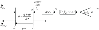
Figure 10: Implementation of a dissipative coupling together with the linear control.

B.3 Models with dispersive coupling $\hat{L}=\sqrt{\kappa}\hat{q}$ and direct measurement feedback

For realization of a dispersive coupling of the form $\hat{L}=\sqrt{\kappa}\hat{q}$, consider the configuration shown in Fig. 11. This configuration consists of a ring cavity with mode $\hat{a}$, an auxiliary ring cavity with mode $\hat{b}$, a $\chi^{(2)}$ nonlinear crystal in which the cavity modes $\hat{a}$ and $\hat{b}$ interact with a classical pump beam, and a beam splitter. The frequency of the auxiliary cavity is matched to half the frequency of the pump beam. The classically pumped nonlinear crystal implements a two-mode squeezing Hamiltonian given by $\hat{H}_{TMS}=\frac{{\rm i}}{2}(\epsilon e^{-{\rm i}\omega_{p}t}\hat{a}^{*}\hat{b}^{*}-\epsilon^{*}e^{{\rm i}\omega_{p}t}\hat{a}\hat{b})$ (where $\epsilon$ is the effective intensity of the classical pump and $\omega_{p}$ is the pump frequency), while the beam splitter implements the Hamiltonian $\hat{H}_{BS}=\alpha\hat{a}^{*}\hat{b}+\alpha^{*}\hat{a}\hat{b}^{*}$ for a complex parameter $\alpha$. Suppose now that $\epsilon$ and $\alpha$ are chosen to satisfy $\epsilon/2={\rm i}\alpha=\Gamma$ for a real constant $\Gamma>0$ (in particular $\alpha=-{\rm i}\Gamma$). Then in a rotating frame at the frequency $\omega_{p}/2$, the overall interaction Hamiltonian between the modes $\hat{a}$ and $\hat{b}$ is thus given by

$$\hat{H}_{\hat{a}\hat{b}}=i\Gamma(\hat{a}^{*}\hat{b}^{*}-\hat{a}\hat{b}-\hat{a}^{*}\hat{b}+\hat{a}\hat{b}^{*}).$$

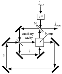
Figure 11: Configuration of two cavities, a two mode squeezer (depicted by the square with an arrow to indicate classical pumping), and a beam splitter, to implement a dispersive coupling of the cavity mode $\hat{a}$ to the field $\hat{B}_{in,t}$ when the second cavity mode $\hat{b}$ is adiabatically eliminated. Note that $\hat{B}_{in,t}$ is phase shifted by 180^∘ before reaching the mirror $M$.

Assume that the coupling coefficient of the mirror $M$ is large such that the mode $\hat{b}$ is heavily damped compared to mode $\hat{a}$ and has much faster dynamics than $\hat{a}$. For simplicity, in the following we will use the formalism of quantum Langevin equations and a formal method to show that the configuration shown implements the dispersive coupling $\hat{L}$ in the reduced dynamics for mode $\hat{a}$ only, after mode $\hat{b}$ is adiabatically eliminated . See NJD08 for a more rigorous derivation using QSDEs and the mathematical theory for adiabatic elimination developed in BvHS07 .

Let $\hat{B}_{in,t}$ be an input field and $\hat{B}_{out,t}$ be an output field coupled to $\hat{b}$ at the mirror $M$ as shown in Fig. 11 and suppose that $M$ has the coupling coefficient $\gamma$. In particular, notice the 180^∘ phase shift in front of $\hat{B}_{in,t}$ before it strikes the mirror. Define $\hat{\eta}$ to be a quantum white noise formally related to $\hat{B}_{in,t}$ as $\hat{B}_{in,t}=\int_{0}^{t}\hat{\eta}(s)ds$ and $\hat{\eta}_{out}$ be the output noise at the mirror $M$ formally related to $\hat{B}_{out,t}$ by $\hat{B}_{out,t}=\int_{0}^{t}\hat{\eta}_{out}(s)ds$. The quantum Langevin equations for the dynamics of $\hat{a}$, $\hat{b}$, and $\hat{\eta}_{out}$ are (Gardiner, , Chapter 5)

$$\dot{\hat{a}} = {\rm i}[\hat{H}_{\hat{a}\hat{b}},\hat{a}]$$ (84)

$$= \Gamma(\hat{b}^{*}-\hat{b}),$$

$$\dot{\hat{b}} = {\rm i}[\hat{H}_{\hat{a}\hat{b}},\hat{b}]-\frac{\gamma}{2}\hat{b}+\sqrt{\gamma}\hat{\eta}$$ (85)

$$= \Gamma(\hat{a}^{*}+\hat{a})-\frac{\gamma}{2}\hat{b}+\sqrt{\gamma}\hat{\eta},$$

$$\hat{\eta}_{out} = \sqrt{\gamma}\hat{b}-\hat{\eta}.$$ (86)

Setting $\dot{\hat{b}}=0$ and solving Eq. (85) for $\hat{b}$ in terms of $\hat{a}^{*}$, $\hat{a}$ and $\hat{\eta}$ we obtain

$$\hat{b}=\frac{2}{\gamma}\left(\Gamma(\hat{a}^{*}+\hat{a})+\sqrt{\gamma}\hat{\eta}\right).$$ (87)

Substituting Eq. (87) into Eqs. (84) and (86) we obtain that the reduced dynamics for $\hat{a}$ only and $\hat{\eta}_{out}$ are given by the following quantum Langevin equations:

$$\dot{\hat{a}} = \Gamma(\hat{b}^{*}-\hat{b})$$ (88)

$$= \frac{2\Gamma}{\sqrt{\gamma}}(-\hat{\eta}+\hat{\eta}^{*}),$$

$$\hat{\eta}_{out} = \frac{2\Gamma}{\sqrt{\gamma}}(\hat{a}+\hat{a}^{*})+\hat{\eta}.$$ (89)

The pair of equations (88) and (89) shows that the reduced system after adiabatic elimination of the mode $\hat{b}$ is a single degree of freedom quantum harmonic oscillator with mode $\hat{a}$ coupled to the field $\hat{B}_{in,t}$ by the linear coupling operator $\hat{L}=2\sqrt{2}\Gamma\hat{q}/\sqrt{\gamma}$, where $\hat{q}=(\hat{a}+\hat{a}^{*})/\sqrt{2}$, producing the output field $\hat{B}_{out,t}=\int_{0}^{t}\hat{\eta}_{out}(s)ds$. By suitably choosing $\Gamma$ and $\gamma$ such that $2\sqrt{2}\Gamma=\sqrt{\kappa\gamma}$ we see that with this scheme it is possible to implement any dispersive coupling of the form $\hat{L}=\sqrt{\kappa}\hat{q}$. Moreover, by placing a pumped nonlinear crystal inside the cavity (pumped with the same frequency $\omega_{p}$) and adding a partially transmitting mirror in the ring cavity of $\hat{a}$ that couples it to a control field, one can easily combine this dispersive coupling together with the quadratic Hamiltonian in Subsection 1 of this Appendix as well as the control shown in Fig. 10.

References

• (1) M. A. Nielsen and I. L. Chuang, Quantum Computation and Quantum Information, (Cambridge University Press, Cambridge, 2000).
• (2) J. I. Cirac, P. Zoller, J. H. Kimble, and H. Mabuchi, Phys. Rev. Lett. 78, 3221 (1997).
• (3) S. J. van Enk, J. I. Cirac, and P. Zoller, Phys. Rev. Lett. 78, 4293 (1997).
• (4) A. S. Parkins and H. J. Kimble, J. Opt. B: Quantum Semiclass. Opt. 1, 496 (1999).
• (5) A. S. Parkins and H. J. Kimble, Phys. Rev. A 61, 052104 (2000).
• (6) C. H. Bennett, G. Brassard, S. Popescu, B. Schumacher, J. A. Smolin, and W. K. Wootters, Phys. Rev. Lett. 76, 722 (1996).
• (7) C. H. Bennett, D. P. DiVincenzo, J. A. Smolin, and W. K. Wootters, Phys. Rev. A 54, 3824 (1996).
• (8) T. Yu and J. H. Eberly, Phys. Rev. Lett. 93, 140404 (2004).
• (9) J. H. Eberly and T. Yu, Science, 316, 27 (2007).
• (10) A. C. Doherty and K. Jacobs, Phys. Rev. A 60, 2700 (1999).
• (11) L. Thomsen, S. Mancini, and H. M. Wiseman, J. Phys. B, 35, 4937 (2002).
• (12) C. Ahn, H. M. Wiseman, and G. J. Milburn, Phys. Rev. A 67, 052310 (2003).
• (13) L. M. Bouten, R. van Handel, and M. R. James, to appear in SIAM Review, arXiv: math/0606118 (2006).
• (14) J. Wang, H. M. Wiseman, and G. J. Milburn, Phys. Rev. A 71, 042309 (2005).
• (15) A. R. R. Carvalho and J. J. Hope, Phys. Rev. A 76, 010301(R) (2007).
• (16) M. Mirrahimi and R. van Handel, SIAM J. Control Optim. 46, 445-467 (2007).
• (17) N. Yamamoto, K. Tsumura, and S. Hara, Automatica 43, 981-992 (2007).
• (18) S. Mancini and H. M. Wiseman, Phys. Rev. A 75, 012330 (2007).
• (19) H. M. Wiseman and G. J. Milburn, Phys. Rev. Lett. 70, 548 (1993).
• (20) H. M. Wiseman, Phys. Rev. A 49, 2133 (1994).
• (21) M. Yanagisawa, Phys. Rev. Lett. 97, 190201 (2006).
• (22) P. Warszawski, H. M. Wiseman, and H. Mabuchi, Phys. Rev. A 65, 023802 (2002).
• (23) P. Warszawski and H. M. Wiseman, J. Opt. B: Quantum Semiclass. Opt. 5, 1 (2003).
• (24) P. Warszawski and H. M. Wiseman, J. Opt. B: Quantum Semiclass. Opt. 5, 15 (2003).
• (25) S. L. Braunstein and P. van Loock, Rev. Mod. Phys. 77, 513 (2005).
• (26) H. J. Carmichael, An open system approach to quantum optics, Springer, Berlin (1993).
• (27) H. J. Carmichael, Phys. Rev. Lett. 70, 2273 (1993).
• (28) C. W. Gardiner and P. Zoller, Quantum Noise, Springer, Berlin (2000).
• (29) J. Gough and M. R. James, arXiv: 0707.0048 (2007).
• (30) R. L. Hudson and K. R. Parthasarathy, Commun. Math. Phys. 93, 301 (1984).
• (31) S. C. Edwards and V. P. Belavkin, arXiv: quant-ph/0506018 (2005).
• (32) H. I. Nurdin, M. R. James, and A. C. Doherty, arXiv:0806.4448 (2008).
• (33) M. R. James, H. I. Nurdin, and I. R. Petersen, to appear in IEEE Trans. Automat. Contr., arXiv:quant-ph/0703150 (2007).
• (34) L. M. Duan, G. Giedke, J. I. Cirac, and P. Zoller, Phys. Rev. Lett. 84, 2722 (2000).
• (35) R. Simon, Phys. Rev. Lett. 84, 2726 (2000).
• (36) G. Vidal and R. F. Werner, Phys. Rev. A 65, 032314 (2002).
• (37) K. Zhou, J. Doyle, and K. Glover, Robust and Optimal Control, Prentice Hall, NJ (1996).
• (38) Z. Ficek and R. Tanas, Phys. Rev. A 77, 054301 (2008).
• (39) M. G. A. Paris, F. Illuminati, A. Serafini, and S. DeSiena, Phys. Rev. A 68, 012314 (2003).
• (40) G. J. Milburn, Quantum Semiclass. Opt. 8, 269 (1996).
• (41) A. C. Doherty, S. M. Tan, A. S. Parkins, and D. F. Walls, Phys. Rev. A 60, 2380 (1999).
• (42) H. M. Wiseman and G. J. Milburn, Phys. Rev. A 47, 642 (1993).
• (43) H. M. Wiseman and A. C. Doherty, Phys. Rev. Lett. 94, 070405 (2005).
• (44) C. D’Helon and M. R. James, Phys. Rev. A 73, 053803 (2006).
• (45) L. Bouten, R. van Handel, and A. Silberfarb, Journal of Functional Analysis 254, 3123 (2008).
• (46) J. Gough and R. van Handel, J. Stat. Phys. 127, 575 (2007).