Practical schemes for the measurement of angular-momentum covariance matrices in quantum optics

Abstract

We develop practical schemes for the measurement of the covariance matrix for intrinsic angular-momentum variables in quantum optics. We particularize this approach to two-beam polarimetry and interferometry, as well as to ensembles of two-level atoms interacting with classical fields. We show the practical advantages of noisy simultaneous measurements.

I Introduction

Angular-momentum variables represent basic observables both in classical and quantum optics, especially in three fundamental areas: polarization, interferometry, and light-matter interaction HL ; be ; yea ; mbe ; cvpe ; asc ; yop ; SZ ; yobs ; pepe . For definiteness, throughout we focus on intrinsic (not orbital) angular momenta. This is for example the case of the Stokes parameters, which provide a complete account of second-order (in complex amplitudes) statistical properties of two-mode polarization and interference. Moreover, spin operators are basic in atomic physics such as in the case of ensembles of two-level atoms described individually as spin 1/2 systems.

The second-order statistics of angular-momentum variables are crucial in diverse areas. This is the case with quantum metrology, where angular-momentum statistics determine the ultimate limit to the resolution of interferometric and spectroscopic measurements HL ; be ; yea . Moreover, angular-momentum covariance matrices enter in the analysis of many-body entanglement mbe , in continuous-variable polarization entanglement cvpe , and for light-mediated detection of atomic-spin correlations asc .

Recently we have proposed an SU(2)-invariant characterization of angular-momentum fluctuations via the diagonalization of the covariance matrix RL07 . Invariance under SU(2) transformations is a desirable property since two states connected by a deterministic SU(2) transformation should be statistically equivalent. Similar invariance ideas are at the heart of current investigations about the coherence between classical vectorial waves cvw .

In this work we develop simple practical schemes to determine experimentally the angular-momentum covariance matrix of a given system in an unknown state. We particularize the method to diverse optical two-mode polarimetric and interferometric configurations, as well as to ensembles of two-level atoms. It is worth stressing that this analysis applies equally well to quantum and classical optics. In the classical domain the situation is much more simple since in principle one can always perform as many simultaneous measurements as desired of any set of observables in accurate copies of the original beam provided by beam splitting, for instance. This idea can be fruitfully translated to the quantum domain in the form of noisy simultaneous measurements of noncommuting angular-momentum components.

In Sec. II we recall basic definitions and results. In Sec. III we present a basic scheme for the measurement of angular-momentum covariance matrices which is particularized to polarimetric, interferometric, and spectroscopic situations. In Sec. IV we present an interferometric noisy simultaneous measurement of angular-momentum components providing a simple and exact practical determination of the covariance matrix with a single experimental configuration. In Sec. V we consider the bright limit in which the angular-momentum covariance matrix becomes a quadrature (or position-linear momentum) covariance matrix.

II Definitions

II.1 Definition and two-mode realization

Let us consider arbitrary dimensionless angular momentum operators $\bm{j}^{t}=(j_{1},j_{2},j_{3})$, where the superscript $t$ denotes matrix transposition. In quantum physics they are defined by the fulfillment of the commutation relations

$$[j_{k},j_{\ell}]=i\sum_{n=1}^{3}\epsilon_{k,\ell,n}j_{n},\qquad[j_{0},\bm{j}]=\bm{0},$$ (1)

where $\epsilon_{k,\ell,n}$ is the fully antisymmetric tensor with $\epsilon_{1,2,3}=1$ and $j_{0}$ is defined by the relation

$$\bm{j}^{2}=j_{0}\left(j_{0}+1\right).$$ (2)

For the sake of completeness we take into account that $j_{0}$ may be an operator. This is the case of two-mode realizations where $j_{0}$ is proportional to the number of photons. In classical optics the situation is similar by replacing commutators by Poisson brackets and Eq. (2) by $\bm{j}^{2}=j^{2}_{0}$ (with $\langle\bm{j}\rangle^{2}\leq\langle j_{0}\rangle^{2}$, where the brackets denote an ensemble average).

In quantum and classical optics two-mode realizations of angular momentum play a relevant position in polarimetry and interferometry. In the quantum case, denoting by $a_{1,2}$ the complex amplitudes operators of two field modes, we get that

$$j_{0}=\frac{1}{2}\left(a^{\dagger}_{1}a_{1}+a^{\dagger}_{2}a_{2}\right), j_{1}=\frac{1}{2}\left(a^{\dagger}_{2}a_{1}+a^{\dagger}_{1}a_{2}\right),$$

$$j_{2}=\frac{i}{2}\left(a^{\dagger}_{2}a_{1}-a^{\dagger}_{1}a_{2}\right), j_{3}=\frac{1}{2}\left(a^{\dagger}_{1}a_{1}-a^{\dagger}_{2}a_{2}\right),$$

satisfy Eqs. (1) and (2) SCH , where the superscript $\dagger$ denotes Hermitian conjugation. In the classical domain $a_{1,2}$ are classical amplitudes so that Hermitian conjugation $a^{\dagger}_{1,2}$ is replaced by complex conjugation $a^{\ast}_{1,2}$.

In polarimetry these are essentially the Stokes variables. The normalized vector $\langle\bm{j}\rangle/\langle j_{0}\rangle$ defines the Poincaré sphere as a suitable representation of polarization states and transformations cvpe ; pepe . These are also basic variables in two-beam interferometry. For example, the third component $j_{3}$ is proportional to the difference of the number of photons between two modes, while $j_{1,2}$ express the coherence between the interfering beams.

II.2 Covariance matrix

The complete second-order statistics of $\bm{j}$ is contained in the $3\times 3$ real symmetric covariance matrix $M$

$$M_{k,\ell}=\frac{1}{2}\left(\left\langle j_{k}j_{\ell}\right\rangle+\left\langle j_{\ell}j_{k}\right\rangle\right)-\left\langle j_{k}\right\rangle\left\langle j_{\ell}\right\rangle,$$ (4)

with $M^{t}=M$ and $M^{\ast}=M$. The alternative definition $M^{\prime}_{k,\ell}=\left\langle j_{k}j_{\ell}\right\rangle-\left\langle j_{k}\right\rangle\left\langle j_{\ell}\right\rangle$ is identical to $M$ in the classical case, while in the quantum domain it provides a complex Hermitian matrix that contains essentially the same information as $M$ RL07 .

The covariance matrix $M$ allows us to compute the variance $(\Delta j_{u})^{2}$ of an arbitrary angular-momentum component $j_{u}=\bm{u}\cdot\bm{j}$, where $\bm{u}$ is any unit real vector,

$$\left(\Delta j_{u}\right)^{2}=\bm{u}^{t}M\bm{u},$$ (5)

as well as the symmetric correlation of two arbitrary components $j_{u}=\bm{u}\cdot\bm{j}$ and $j_{v}=\bm{v}\cdot\bm{j}$, where $\bm{u}$ and $\bm{v}$ are unit real vectors,

$$\frac{1}{2}\left(\langle j_{u}j_{v}\rangle+\langle j_{v}j_{u}\rangle\right)-\langle j_{u}\rangle\langle j_{v}\rangle=\bm{v}^{t}M\bm{u}=\bm{u}^{t}M\bm{v}.$$ (6)

Since $M$ is real and symmetric, the transformation that renders $M$ diagonal is a rotation matrix $R_{d}$

$$M=R^{t}_{d}\pmatrix{(\Delta J_{1})^{2}&0&0\cr 0&(\Delta J_{2})^{2}&0\cr 0&0&(\Delta J_{3})^{2}}R_{d}.$$ (7)

The eigenvalues of $M$, $(\Delta J_{k})^{2}$, $k=1,2,3$, are the variances of the components $J_{k}=\bm{u}_{k}\cdot\bm{j}$, where $\bm{u}_{k}$ are the three real orthonormal eigenvectors of $M$

$$M\bm{u}_{k}=(\Delta J_{k})^{2}\bm{u}_{k}.$$ (8)

Following standard nomenclature in statistics we refer to $\bm{J}$ and $\Delta\bm{J}$ as principal components and principal variances, respectively. We stress that both $\bm{J}$ and $\Delta\bm{J}$ depend on the system state. The principal variances provide an SU(2) invariant characterization of angular momentum fluctuations RL07 .

II.3 SU(2) invariance

Throughout, by SU(2) invariance we mean the statistical equivalence between states connected by unitary deterministic transformation generated by $\bm{j}$

$$U=\exp\left(i\theta\bm{u}\cdot\bm{j}\right),$$ (9)

where $\theta$ is a real parameter and $\bm{u}$ is a unit three-dimensional real vector. It can be seen (for example, by using the $j_{0}=1/2$ representation) that the action of $U$ on $\bm{j}$ is a rotation $R$ of angle $\theta$ and axis $\bm{u}$ CS

$$U^{\dagger}\bm{j}U=R\bm{j},\quad U^{\dagger}j_{0}U=j_{0},$$ (10)

where the $3\times 3$ real matrix $R$ is

$$R_{k,\ell}=\frac{1}{2}\textrm{tr}\left(\sigma_{\ell}\mathcal{U}^{\dagger}\sigma_{k}\mathcal{U}\right),$$ (11)

with

$$\mathcal{U}=\exp\left(i\theta V\right),\quad V=\frac{1}{2}\sum_{k=1}^{3}u_{k}\sigma_{k},$$ (12)

where $k,\ell=1,2,3$, $\sigma_{1,2,3}$ are the Pauli matrices and it holds that $R^{t}=R^{-1}$, and $\mathcal{U}^{\dagger}=\mathcal{U}^{-1}$.

The SU(2) invariance of principal variances holds because under any SU(2) transformation $M$ transforms as $M\rightarrow RMR^{t}$. Therefore, the covariance matrix $RMR^{t}$ associated with the transformed state has the same principal variances as the covariance matrix $M$ associated with the original state.

In other words, the SU(2) invariance is just the mathematical statement corresponding to the fact that the conclusions which one could draw from an angular momentum measurement must be independent of which set of three orthogonal angular momentum components one chooses.

In the case of the two-mode bosonic realizations (II.1) we have

$$\bm{b}=U^{\dagger}\bm{a}U=\mathcal{U}\bm{a},\quad U=\exp\left(i\theta\bm{a}^{\dagger}V\bm{a}\right),$$ (13)

where $\mathcal{U}$ and $V$ are in Eq. (12) and $\bm{a}^{t}=(a_{1},a_{2})$ and $\bm{b}^{t}=(b_{1},b_{2})$ are the original and transformed complex amplitudes, respectively. In this case SU(2) transformations describe basic lossless polarization and interference elements, such as beam splitters, phase plates, two-beam interferometers, Faraday rotators, etc. HL ; be ; yea ; cvpe ; yop ; yobs .

III Practical determination of the covariance matrix

The complete determination of the covariance matrix in a given basis of components $\bm{j}^{t}=(j_{1},j_{2},j_{3})$ can be achieved by measurement of the variances of the six operators

$$j_{1\pm 2}=\frac{1}{\sqrt{2}}\left(j_{1}\pm j_{2}\right),$$

$$j_{1\pm 3}=\frac{1}{\sqrt{2}}\left(j_{1}\pm j_{3}\right),$$

$$j_{2\pm 3}=\frac{1}{\sqrt{2}}\left(j_{2}\pm j_{3}\right).$$ (14)

More specifically, since (respecting the quantum lack of commutation)

$$j^{2}_{k\pm\ell}=\frac{1}{2}\left(j_{k}^{2}+j_{\ell}^{2}\pm j_{k}j_{\ell}\pm j_{\ell}j_{k}\right),$$ (15)

we get that the nondiagonal matrix elements $M_{k,\ell}$, $k\neq\ell$, are given by

$$M_{k,\ell}=\frac{1}{2}\left[\left(\Delta j_{k+\ell}\right)^{2}-\left(\Delta j_{k-\ell}\right)^{2}\right].$$ (16)

For the diagonal elements we have

$$M_{3,3}= \left(\Delta j_{3}\right)^{2}=\frac{1}{2}\left[\left(\Delta j_{1+3}\right)^{2}+\left(\Delta j_{1-3}\right)^{2}+\left(\Delta j_{2+3}\right)^{2}\right.$$ (17)

$$\left.+\left(\Delta j_{2-3}\right)^{2}-\left(\Delta j_{1+2}\right)^{2}-\left(\Delta j_{1-2}\right)^{2}\right],$$

and similarly for $\Delta j_{1}$ and $\Delta j_{2}$ by cyclic permutations of the indices.

Note that $M$ has just six independent components because of reality and symmetry, which agrees with the above number of independent measured variances. The six operators (III) are not, strictly speaking, independent since we have, for example,

$$j_{2+3}=j_{1+2}-j_{1-3},\quad j_{2-3}=j_{1+2}-j_{1+3}.$$ (18)

Nevertheless, measurement of the components $j_{2\pm 3}$ is necessary to derive all $j_{k}j_{\ell}$ correlations exclusively in terms of variances.

When one of the components of $\bm{j}$, say $j_{3}$, is a principal component, the process is much more simple since we know in advance that all the correlations between $j_{3}$ and $j_{1}$, $j_{2}$ vanish. Then, only four variances are necessary: namely $\Delta j_{1}$, $\Delta j_{2}$, $\Delta j_{3}$, and $\Delta j_{1+2}$ for example.

The measured components $j_{p\pm q}$ can be related with the original ones $j_{\ell}$ by simple SU(2) transformations of the form

$$U_{k,\pm m}=\exp\left(i\theta_{\pm m}j_{k}\right),$$ (19)

with $\theta_{\pm m}=\pm\pi/m$ and $m=2,4$, which produce rotations of angles $\pi/2$ and $\pi/4$ around the axis $j_{k}$. This is useful because $U_{k,\pm 4}$ transform the measurement of the components $j_{\ell}$ in the transformed state into the measurement of the operators $j_{p\pm q}$ in the original state, while $U_{k,\pm 2}$ transform the components $j_{\ell}$ among themselves. The proper use of these transformations is illustrated by the following particular cases.

III.1 Polarimetry

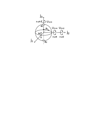
Figure 1: Poincaré sphere illustrating polarization states (circular at the poles and linear at the equator) and the action of the transformations (III.1).

Polarization states and transformations can be properly represented in the Poincaré sphere, as illustrated in Fig. 1. For definiteness we consider $a_{1,2}$ in Eq. (II.1) as the amplitudes of circularly polarized modes,

$$a_{1}=\frac{1}{\sqrt{2}}\left(a_{x}+ia_{y}\right),\quad a_{2}=\frac{1}{\sqrt{2}}\left(a_{x}-ia_{y}\right),$$ (20)

where $a_{x,y}$ are the complex amplitudes of modes linearly polarized along the Cartesian axes $x$ and $y$. As customary, the south and north poles in axis $j_{3}$ of the Poincaré sphere represent circularly polarized light, while linear polarizations of different azimuths are distributed along the equator, with linear polarization along the Cartesian axes $x$ and $y$ located at the antipodal points of the axis $j_{1}$ (i.e., $j_{1}=\pm j_{0}$).

Figure 2: Illustration of the scheme for the polarimetric measurement of the covariance matrix.

The most simple polarization measurement is the measurement of $j_{1}=(a^{\dagger}_{x}a_{x}-a^{\dagger}_{y}a_{y})/2$ as the difference between the field intensities after a polarizing beam splitter, as illustrated in Fig. 2. In this case the transformations (19) correspond to phase plates and Faraday rotations placed before the polarizing beam splitter that transform the measurement of $j_{1}$ in the output fields into the measurement of $j_{k\pm\ell}$ in the input fields. More specifically,

$$j_{1\pm 2}=U_{3,\pm 4}^{\dagger}j_{1}U_{3,\pm 4},$$

$$j_{1\pm 3}=U_{2,\mp 4}^{\dagger}j_{1}U_{2,\mp 4},$$

$$j_{2\pm 3}=U_{2,\mp 2}^{\dagger}U_{3,4}^{\dagger}j_{1}U_{3,4}U_{2,\mp 2}.$$ (21)

The transformations $U_{3,\pm 4}$ are Faraday rotations producing a phase different shift of $\pm\pi/4$ between dextro and levo circularly polarized modes. This produces a rotation of angle $\pm\pi/8$ of the azimuth of linearly polarized light, which is a rotation of the Poincaré sphere of angle $\pm\pi/4$ along the north-south axis. On the other hand, the transformations $U_{2,\pm 2}$ and $U_{2,\pm 4}$ can be implemented by phase plates introducing phase-difference shifts of $\pm\pi/2$ and $\pm\pi/4$, respectively, the phase-plate axes forming $\pm\pi/4$ with the Cartesian axes $x$ and $y$.

III.2 Two-beam interferometry

Two-beam interferometry can be embedded in this same framework by considering that the complex amplitudes $a_{1,2}$ represent two interfering modes with the same polarization state and propagating along different directions. In this case, the simplest measurement is $j_{3}$, since it represents the difference of intensities between the two waves $a_{1,2}$. Otherwise, the same relations (III.1) hold simply by the cyclic permutation $(1,2,3)\rightarrow(3,1,2)$ for the indices $k$ and $\ell$ in $j_{k\pm\ell}$, $j_{k}$, and $U_{k,\pm m}$.

The transformations (19) represent in general lossless beam splitters and phase shifts. In terms of input-output relations (13) we get for $U_{2,\pm m}$ the following unitary matrices relating input and output complex amplitudes

$$\mathcal{U}_{2,\pm m}=\pmatrix{\cos(\theta_{\pm}/2)&\sin(\theta_{\pm}/2)\cr-\sin(\theta_{\pm}/2)&\cos(\theta_{\pm}/2)},$$ (22)

while for $U_{1,\pm m}$,

$$\mathcal{U}_{1,\pm m}=\pmatrix{\cos(\theta_{\pm}/2)&i\sin(\theta_{\pm}/2)\cr i\sin(\theta_{\pm}/2)&\cos(\theta_{\pm}/2)}.$$ (23)

In Fig. 3 we illustrate how these transformations may be implemented with very simple elements such as symmetric beam splitters (SBS) and phase-difference shifts (PDS), described by the unitary matrices

$$N_{\textrm{SBS}} = \frac{1}{\sqrt{2}}\pmatrix{1&i\cr i&1},$$

$$N_{\textrm{PDS}} = \pmatrix{\exp{(i\phi)}&0\cr 0&\exp{(-i\phi)}}.$$ (24)

For $\mathcal{U}_{2,\pm m}$ we have the parameters $\varphi=\pi/2$, $\phi=\theta_{\pm m}/2-\pi/2$, and $\delta=0$, while for $\mathcal{U}_{1,\pm m}$ the parameters are $\varphi=\delta=\pi/4$ and the same $\phi=\theta_{\pm m}/2-\pi/2$.

Figure 3: Illustration of the interferometric realization of the transformations (22) and (23) using symmetric beam splitters (SBS) and phase-difference shifts (PDS) exclusively.

III.3 Two-level atoms

In this case the physical situation corresponds to a collection of $N$ two-level atoms (with ground $|g\rangle$ and excited $|e\rangle$ levels) interacting with a classical field $\bm{E}=\bm{E_{0}}\cos(\omega t)$. By assuming that the coupling between atoms can be neglected the total Hamiltonian is given by the sum of individual Hamiltonians (in units $\hbar=1$ for simplicity),

$$H=\sum_{k=1}^{N}h_{k},$$ (25)

being

$$h_{k}=\frac{\omega_{0}}{2}\sigma_{3}^{(k)}-\Omega\left[\sigma_{-}^{(k)}+\sigma_{+}^{(k)}\right]\cos(\omega t),$$ (26)

where, for each atom $k$,

$$\sigma_{3}=|e\rangle\langle e|-|g\rangle\langle g|,\quad\sigma_{-}=\sigma_{+}^{\dagger}=|g\rangle\langle e|$$ (27)

are the corresponding Pauli and ladder matrices with $\sigma_{\pm}=(\sigma_{1}\pm i\sigma_{2})/2$. The first term in Eq. (26) is the free-evolution Hamiltonian for each atom and the second one is the coupling with the classical field at dipolar approximation. The Rabi frequency $\Omega=\langle g|\hat{\bm{d}}|e\rangle\cdot\bm{E_{0}}$ has been assumed to be real. On the regimen $\omega\simeq\omega_{0}\gg\Omega$ is usually used to consider the rotating wave approximation by neglecting the counter-rotating terms $\sigma_{+}\exp(i\omega t)$ and $\sigma_{-}\exp(-i\omega t)$ in the above Hamiltonians SZ

$$h_{k}\simeq \frac{\omega_{0}}{2} \sigma_{3}^{(k)}-\frac{\Omega}{2}\left[\sigma_{-}^{(k)}\exp(i\omega t)+\sigma_{+}^{(k)}\exp(-i\omega t)\right]$$

$$= \frac{\omega_{0}}{2} \sigma_{3}^{(k)}-\frac{\Omega}{2}\left[\sigma_{1}^{(k)}\cos(\omega t)+\sigma_{2}^{(k)}\sin(\omega t)\right].$$ (28)

From Eqs. (25) and (III.3) the total Hamiltonian can be written in terms of the total angular momentum $\bm{j}=\sum_{k}\bm{\sigma}^{(k)}/2$ as

$$H=\omega_{0}j_{3}-\Omega\left[j_{1}\cos(\omega t)+j_{2}\sin(\omega t)\right]=U_{3}^{\dagger}\left[\omega_{0}j_{3}-\Omega j_{1}\right]U_{3},$$ (29)

where $U_{3}=\exp(i\omega tj_{3})$ is a rotation around the $j_{3}$ axis.

It is customary to change the picture by the unitary transform $U_{3}=\exp(i\omega tj_{3})$ in order to remove the time dependence of the Hamiltonian

$$|\psi(t)\rangle\rightarrow|\tilde{\psi}(t)\rangle=U_{3}|\psi(t)\rangle,$$ (30)

with $|\tilde{\psi}(0)\rangle=|\psi(0)\rangle$. The time-evolution equation in this picture is

$$i\frac{d}{dt}|\tilde{\psi}(t)\rangle=\left[(\omega_{0}-\omega)j_{3}-\Omega j_{1}\right]|\tilde{\psi}(t)\rangle,$$ (31)

so the operator $U(t_{2},t_{1})$ performing the time evolution between $t_{1}=0$ and $t_{2}=t$ in the Schrödinger picture is

$$U(t,0)=\exp(-i\omega tj_{3})\exp\{-i\left[(\omega_{0}-\omega)j_{3}-\Omega j_{1}\right]t\}.$$ (32)

This operator reduces to a very simple product of SU(2) transformations when the radiation field is in resonance $\omega=\omega_{0}$:

$$U_{\mathrm{res}}(t,0)=\exp(-i\omega_{0}tj_{3})\exp(i\Omega tj_{1}).$$ (33)

On the other hand, if the external field is switched off $(\Omega=0)$, the free evolution is given by

$$U_{\mathrm{free}}(t)=\exp(-i\omega_{0}tj_{3}).$$ (34)

Therefore, in this case the transformations $U_{k\pm m}$ are obtained by combining time intervals of resonance pulses and free evolution, as is used in Ramsey spectroscopy Rm .

As in the interferometric case above, the simplest measurement is $j_{3}$ again, this is the difference of populations between the two levels of the atoms (nevertheless, see Ref. asc for other light-mediated atomic-spin measuring schemes). More explicitly $U_{2,\pm m}$ can be achieved as

$$U_{2,\pm m}=U_{\mathrm{free}}(t_{\pi/2}-t_{\pm m})U_{\mathrm{res}}(t_{\pm m},0)U_{\mathrm{free}}(t_{-\pi/2}),$$ (35)

with $\omega_{0}t_{\pm\pi/2}=\pm\pi/2\;\mathrm{mod}(2\pi)$ and, in order to deal always with positive time intervals, $\Omega t_{m}=\pi/m$ and $\Omega t_{-m}=(2m-1)\pi/m$. Similarly $U_{1,\pm m}$ can be achieved as

$$U_{1,\pm m}=U_{\mathrm{free}}(t_{2\pi}-t_{\pm m})U_{\mathrm{res}}(t_{\pm m},0),$$ (36)

with $\omega_{0}t_{2\pi}=2\pi\;\mathrm{mod}(2\pi)$ and the same $t_{\pm m}$ above. We stress that the $\mathrm{mod}(2\pi)$ freedom should be used to obtain always positive time intervals.

In these equations the following relation is useful

$$\exp(i\varphi j_{2})=\exp\left(-i\frac{\pi}{2}j_{3}\right)\exp(i\varphi j_{1})\exp\left(i\frac{\pi}{2}j_{3}\right),$$ (37)

which can be derived from the relations in Sec. IIC for $\theta=\pi/2$ and $V=\sigma_{3}/2$, so that the rotation matrix in Eqs. (10) and (11) becomes

$$R=\pmatrix{0&1&0\cr-1&0&0\cr 0&0&1}.$$ (38)

IV Simultaneous measurements

In this section we show that an interferometric noisy simultaneous measurement of the three components of $\bm{j}$ provides a simple and exact determination of the covariance matrix with a single apparatus (similar schemes may be developed for the other contexts). The subject of simultaneous measurements of noncommuting observables has a long history, being closely related to basic issues of quantum theory such as generalized measurements, state reconstruction, complementarity, uncertainty relations, etc. GM . In our case we consider the 12-port scheme illustrated in Fig. 4 YP ; RI00 . The two input signal modes are $a_{1}$ and $a_{2}$, while the input modes $a_{10}$, $a_{20}$, $a^{\prime}_{10}$ and $a^{\prime}_{20}$ are auxiliary modes always in the vacuum state.

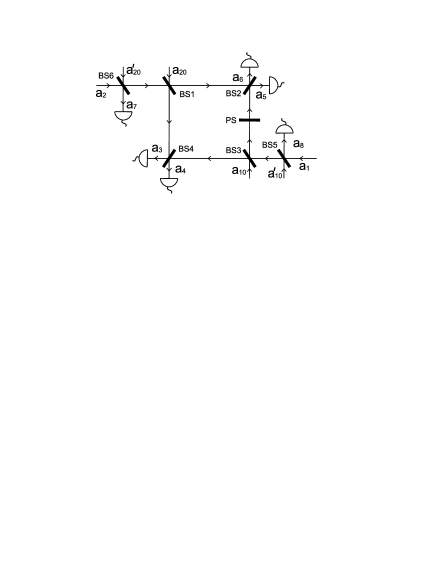
Figure 4: Illustration of the 12-port scheme.

For definiteness and to simplify formulas let us consider that beam splitters BS1, BS2, BS3 and BS4 are 50% with real transmission and reflection coefficients and a $\pi$ phase change in the upper side reflections. BS5 and BS6 are identical with real transmission $t$ and reflection $r$ coefficients, with $t\neq r$, and a $\pi$ phase shift in the upper side reflections. Finally PS is a $\pi/2$ phase shift. The relation between the input and output complex amplitudes is YP

$$a_{3} = \frac{1}{2}\left(ta_{1}-ta_{2}+a_{10}-a_{20}+ra^{\prime}_{10}+ra^{\prime}_{20}\right),$$

$$a_{4} = \frac{1}{2}\left(ta_{1}+ta_{2}+a_{10}+a_{20}+ra^{\prime}_{10}-ra^{\prime}_{20}\right),$$

$$a_{5} = \frac{1}{2}\left(-ita_{1}+ta_{2}+ia_{10}-a_{20}-ira^{\prime}_{10}-ra^{\prime}_{20}\right),$$

$$a_{6} = \frac{1}{2}\left(-ita_{1}-ta_{2}+ia_{10}+a_{20}-ira^{\prime}_{10}+ra^{\prime}_{20}\right),$$

$$a_{7} = ra_{2}+ta^{\prime}_{20},$$

$$a_{8} = -ra_{1}+ta^{\prime}_{10}.$$ (39)

In the classical domain the vacuum state implies that $a_{10}=a_{20}=a^{\prime}_{10}=a^{\prime}_{20}=0$, so we have the noiseless simultaneous measurement of all the components (II.1) via the detection of the six output intensities $I_{j}=a^{\ast}_{j}a_{j}$, $j=3,\ldots,8$, in the form

$$j_{0}=\frac{1}{2}\sum_{j=3}^{8}I_{j}, j_{1}=\frac{1}{t^{2}}\left(I_{4}-I_{3}\right),$$

$$j_{2}=\frac{1}{t^{2}}\left(I_{6}-I_{5}\right), j_{3}=\frac{1}{2r^{2}}\left(I_{8}-I_{7}\right).$$ (40)

With this we can compute the whole covariance matrix $M$ by determining the variances and correlations between the output intensities $I_{j}$.

In the quantum case the amplitudes of the auxiliary modes $a_{10}$, $a_{20}$, $a^{\prime}_{10}$ and $a^{\prime}_{20}$ cannot be taken as zero since the complex amplitude of the vacuum fluctuates. In other words, simultaneous exact measurements of noncommuting operators are forbidden by commutation relations. Nevertheless, it is still possible to extract useful and reliable information from simultaneous noisy measurements. To this end let us define the commuting measured observables

$$\tilde{j}_{1}=\frac{1}{t^{2}}\left(a^{\dagger}_{4}a_{4}-a^{\dagger}_{3}a_{3}\right),$$

$$\tilde{j}_{2}=\frac{1}{t^{2}}\left(a^{\dagger}_{6}a_{6}-a^{\dagger}_{5}a_{5}\right),$$

$$\tilde{j}_{3}=\frac{1}{2r^{2}}\left(a^{\dagger}_{8}a_{8}-a^{\dagger}_{7}a_{7}\right),$$ (41)

as providing a noisy joint measurement of the operators (II.1). We do not include $j_{0}$ because this measurement is actually exact and noiseless because of conservation of total photon number between the input and output (the auxiliary modes are in an eigenstate of the number operator).

In Ref. YP it was shown that for the mean values and variances we have

$$\langle\tilde{\bm{j}}\rangle=\langle\bm{j}\rangle$$ (42)

and

$$\left(\Delta\tilde{j}_{1}\right)^{2} = \left(\Delta j_{1}\right)^{2}+\frac{1+r^{2}}{2t^{2}}\langle j_{0}\rangle,$$

$$\left(\Delta\tilde{j}_{2}\right)^{2} = \left(\Delta j_{2}\right)^{2}+\frac{1+r^{2}}{2t^{2}}\langle j_{0}\rangle,$$

$$\left(\Delta\tilde{j}_{3}\right)^{2} = \left(\Delta j_{3}\right)^{2}+\frac{t^{2}}{2r^{2}}\langle j_{0}\rangle,$$ (43)

so that the diagonal terms of the covariance matrix $\Delta j_{1,2,3}$ can be determined simply and exactly from $\Delta\tilde{j}_{1,2,3}$ and $\langle j_{0}\rangle$. Concerning the nondiagonal terms, it can be seen that the following exact relations hold for all $k\neq\ell$:

$$\langle\tilde{j}_{\ell}\tilde{j}_{k}\rangle=\langle\tilde{j}_{k}\tilde{j}_{\ell}\rangle=\langle:j_{\ell}j_{k}:\rangle=\frac{1}{2}\langle\left(j_{k}j_{\ell}+j_{\ell}j_{k}\right)\rangle,$$ (44)

where $:\;:$ denotes normal ordering. To derive this last relation it can be taken into account that $a^{\dagger}_{k}a_{k}a^{\dagger}_{\ell}a_{\ell}=a^{\dagger}_{k}a^{\dagger}_{\ell}a_{k}a_{\ell}$ for $k\neq\ell$ in order to express $\tilde{j}_{\ell}\tilde{j}_{k}$ in normal order. This is useful since this automatically removes the operators of the auxiliary modes in the vacuum state, leading to $\langle\tilde{j}_{\ell}\tilde{j}_{k}\rangle=\langle:j_{\ell}j_{k}:\rangle$. Then, the last equality in Eq. (44) can be proved by direct computation.

Therefore we get that the statistics of $\tilde{\bm{j}}$ allow one to determine the exact mean values and the covariance matrix for $\bm{j}$. The variances of $\tilde{\bm{j}}$ present an excess of fluctuations caused by the vacuum in the auxiliary modes that can be easily subtracted or compensated. This is particularly simple for $t=\sqrt{2/3}$, $r=\sqrt{1/3}$, since in such a case

$$M=\tilde{M}-\langle j_{0}\rangle\mathcal{I},$$ (45)

where $M$ and $\tilde{M}$ are the correlation matrices for the $\bm{j}$ and $\tilde{\bm{j}}$ operators, respectively, and $\mathcal{I}$ is the $3\times 3$ identity matrix.

It is worth stressing the simplicity of this method since it provides complete information via the measurement of just four observables ($\tilde{\bm{j}}$, $j_{0}$) instead of the six observables of the general method in Eq. (III). Moreover, the four observables ($\tilde{\bm{j}}$, $j_{0}$) are measured in a single experimental arrangement.

The above relations (44) can be regarded as a correspondence between classical variables (the outputs of measuring $\tilde{\bm{j}}$) and quantum mechanical operators $\bm{j}$. In particular, Eq. (44) is actually an angular momentum version of the Wigner W and Terlesky-Margenau-Hill TMH correspondences between products of classical variables and symmetric operator orderings.

Similar schemes may be developed for the polarimetric context. The same interferometric scheme above is valid if the signal modes $a_{1,2}$ are the polarization components $a_{x,y}$. A more polarimetric scheme allowing the noisy simultaneous measurement of $j_{1}$, $j_{2}$, and $j_{3}$ is outlined in Fig. 5. The two beam splitters BS provide three copies of the original beam by mixing with the vacuum, which are directed to three detectors $D$ that are essentially of the form of the $j_{1}$ measuring scheme in Fig. 2. The transformations $U_{2,2}$ and $U_{3,2}$ placed in front of them transform the measurement of $j_{1}$ into measurements of $j_{3}$ and $j_{2}$.

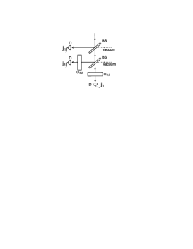
Figure 5: Illustration of a practical scheme for the noisy simultaneous measurement of $j_{1}$, $j_{2}$, and $j_{3}$ in a polarimetric context.

V Bright limit

Focusing on the bosonic realization, when the state of one of the modes is known, the above measuring schemes provide information about the statistical properties of the other mode. Let us examine this issue by considering for definiteness that the system state factorizes $\rho=\rho_{1}\otimes\rho_{2}$, being $\rho_{1}=|\alpha\rangle\langle\alpha|$, where $|\alpha\rangle$ is a coherent state $a_{1}|\alpha\rangle=\alpha|\alpha\rangle$ with real $\alpha$ for simplicity. In such a case we have

$$\langle j_{1}\rangle=\alpha\langle X\rangle,\quad\langle j_{2}\rangle=\alpha\langle Y\rangle,\quad\langle j_{3}\rangle=\frac{1}{2}\left(\alpha^{2}-\langle n\rangle\right),$$ (46)

where $X$ and $Y$ are the quadrature operators of mode $a_{2}$,

$$X=\frac{1}{2}\left(a^{\dagger}_{2}+a_{2}\right),\quad Y=\frac{i}{2}\left(a^{\dagger}_{2}-a_{2}\right),$$ (47)

and $n=a^{\dagger}_{2}a_{2}$ is the number operator. Concerning the covariance matrix we have the following exact series in powers of $\alpha$, valid for any $\alpha$,

$$M=\alpha^{2}M_{2}+\alpha M_{1}+M_{0},$$ (48)

with

$${\scriptsize M_{2}=\pmatrix{\left(\Delta X\right)^{2}&\frac{1}{2}\langle\left(XY+YX\right)\rangle-\langle X\rangle\langle Y\rangle&0\cr\frac{1}{2}\langle\left(XY+YX\right)\rangle-\langle X\rangle\langle Y\rangle&\left(\Delta Y\right)^{2}&0\cr 0&0&\frac{1}{4}}},$$ (49)

$$M_{1}=\frac{1}{4}\pmatrix{0&0&f(X)\cr 0&0&f(Y)\cr f(X)&f(Y)&0},$$ (50)

with $f(A)=\langle A\rangle+2\langle n\rangle\langle A\rangle-\langle\left(An+nA\right)\rangle$ and

$$M_{0}=\frac{1}{4}\pmatrix{\langle n\rangle&0&0\cr 0&\langle n\rangle&0\cr 0&0&\left(\Delta n\right)^{2}}.$$ (51)

In the bright limit $\alpha\rightarrow\infty$ the $\alpha$-leading term in Eq. (48) is $M_{2}$ so that the angular-momentum covariance matrix becomes essentially the quadrature covariance matrix of mode $a_{2}$. This is because in such a limit $X$ and $Y$ become the Cartesian coordinates of the plane tangent to the Poincaré sphere at point $\langle\bm{j}\rangle/\langle j_{0}\rangle\simeq(0,0,1)$ LK . In the same conditions we can consider the bright limit of the 12-port detection scheme in Sec. IV, where mode $a_{1}$ plays the role of the local oscillator. When the local oscillator is in a coherent state $|\alpha\rangle$ with $\alpha\rightarrow\infty$ we have

$$\left(\Delta\tilde{j}_{1}\right)^{2}\simeq\alpha^{2}\left[\left(\Delta X\right)^{2}+\frac{1+r^{2}}{4t^{2}}\right],$$

$$\left(\Delta\tilde{j}_{2}\right)^{2}\simeq\alpha^{2}\left[\left(\Delta Y\right)^{2}+\frac{1+r^{2}}{4t^{2}}\right],$$

$$\langle\tilde{j_{1}}\tilde{j_{2}}\rangle=\langle\tilde{j_{2}}\tilde{j_{1}}\rangle=\frac{\alpha^{2}}{2}\langle\left(XY+YX\right)\rangle.$$ (52)

This agrees well with Eq. (49), as well as with previous analyses of the bright limit of multi-port homodyne detection BL . Analyses of homodyne detection with finite local oscillator are also available YA .

Finally we point out that these results are valid in the general case beyond two-mode bosonic realizations. This holds via the idea of group contraction that applies when the state of the system remains in a small enough region of the Poincaré sphere that can be well approximated by the tangent plane CS .

VI Conclusions

We have provided some general schemes for the practical determination of angular-momentum covariance matrices in different contexts. They allow us to determine a global and SU(2)-invariant characterization of angular-momentum fluctuations via principal components. This can be of interest, for example, for unambiguous, reference-free characterization of SU(2) squeezing with applications in quantum metrology, detection of many-body and continuous-variable entanglement, and light-mediated detection of atomic-spin correlations.

In particular, we have shown that this task can be accomplished in an exact and simple way by noisy simultaneous measurement of angular-momentum components. This provides complete information via the measurement of just four observables, instead of the six observables required by the general method. Moreover, they are measured in a single experimental arrangement.

It is worth stressing the simplicity of this scheme. The minimum number of measured observables required to determine the principal variances is three provided we know in advance the principal components. Just by adding a fourth measurement we no longer need to know the principal components, since we can gather enough information to determine the whole covariance matrix. This includes at once complete information about principal components, principal variances, and the variances of angular-momentum components along arbitrary directions.

References

- (1) B. Yurke, S. L. McCall, and J. R. Klauder, Phys. Rev. A 33, 4033 (1986); M. Hillery and L. Mlodinow, ibid. 48, 1548 (1993); M. J. Holland and K. Burnett, Phys. Rev. Lett. 71, 1355 (1993); C. Brif and A. Mann, Phys. Rev. A 54, 4505 (1996); J. J. Bollinger, W. M. Itano, D. J. Wineland, and D. J. Heinzen, Phys. Rev. A 54, R4649 (1996); S. F. Huelga, C. Macchiavello, T. Pellizzari, A. K. Ekert, M. B. Plenio, and J. I. Cirac, Phys. Rev. Lett. 79, 3865 (1997); T. Nagata, R. Okamoto, J. L. O’Brien, K. Sasaki, and S. Takeuchi, Science 316, 726 (2007).
- (2) Y. Castin and J. Dalibard, Phys. Rev. A 55, 4330 (1997); J. A. Dunningham and K. Burnett, ibid. 61, 065601 (2000); 70, 033601 (2004); V. Meyer, M. A. Rowe, D. Kielpinski, C. A. Sackett, W. M. Itano, C. Monroe, and D. J. Wineland, Phys. Rev. Lett. 86, 5870 (2001).
- (3) D. J. Wineland, J. J. Bollinger, W. M. Itano, and D. J. Heinzen, Phys. Rev. A 50, 67 (1994).
- (4) A. Sørensen, L.-M. Duan, J. I. Cirac, and P. Zoller, Nature (London) 409, 63 (2001); G. Tóth, Phys. Rev. A 69, 052327 (2004); A. R. Usha Devi, M. S. Uma, R. Prabhu, and Sudha, Int. J. Mod. Phys. B 20, 1917 (2006); A. R. Usha Devi, M. S. Uma, R. Prabhu, and A. K. Rajagopal, Phys. Lett. A 364, 203 (2007); A. R. Usha Devi, R. Prabhu, and A. K. Rajagopal, Phys. Rev. Lett. 98, 060501 (2007); G. Tóth, Ch. Knapp, O. Gühne, and H. J. Briegel, ibid. 99, 250405 (2007); O. Gühne P. Hyllus, O. Gittsovich, and J. Eisert, ibid. 99, 130504 (2007); O. Gittsovich, O. Gühne, P. Hyllus, and J. Eisert, e-print arXiv: quant-ph/0803.0757; G. Tóth, Ch. Knapp, O. Gühne, and H. J. Briegel, e-print arXiv: quant-ph/0806.1048.
- (5) N. Korolkova, G. Leuchs, R. Loudon, T. C. Ralph, and Ch. Silberhorn, Phys. Rev. A 65, 052306 (2002); N. Korolkova and R. Loudon, ibid. 71, 032343 (2005).
- (6) K. Eckert, O. Romero-Isart, M. Rodriguez, M. Lewenstein, E. S. Polzik, and A. Sanpera, Nature Phys. 4, 50 (2008); I. de Vega, J. I. Cirac, and D. Porras, Phys. Rev. A 77, 051804 (2008).
- (7) A. Luis and L. L. Sánchez-Soto, in Progress in Optics, edited by E. Wolf (Elsevier, Amsterdam, 2000), Vol. 41, p. 421, and references therein.
- (8) C. Cohen-Tannoudji, J. Dupont-Roc, and G. Grynberg, Atom-Photon Interactions. (John Wiley & Sons, New York, 1998); M. O. Scully and M. S. Zubairy, Quantum Optics (Cambridge University Press, Cambridge, England, 1997).
- (9) A. Luis and L. L. Sánchez-Soto, Quantum Semiclassic. Opt. 7, 153 (1995).
- (10) J. J. Gil, Eur. Phys. J. Appl. Phys. 40, 1 (2007).
- (11) A. Rivas and A. Luis, Phys. Rev. A 77, 022105 (2008).
- (12) J. Tervo, T. Setälä, and A. T. Friberg, Opt. Express 11, 1137 (2003); J. Tervo, T. Setälä, and A. T. Friberg, J. Opt. Soc. Am. A 21, 2205 (2004); P. Réfrégier and F. Goudail, Opt. Express 13, 6051 (2005); A. Luis, J. Opt. Soc. Am. A 24, 1063 (2007); F. Gori, M. Santarsiero, and R. Borghi, Opt. Lett. 32, 588 (2007); P. Réfrégier, J. Math. Phys. 48, 033303 (2007).
- (13) J. Schwinger, Quantum Theory of Angular Momentum (Academic Press, New York, 1965).
- (14) F. T. Arecchi, E. Courtens, R. Gilmore, and H. Thomas, Phys. Rev. A 6, 2211 (1972).
- (15) N. F. Ramsey, Molecular Beams (Oxford University Press, New York, 1985); Rev. Mod. Phys. 62, 541 (1990).
- (16) H. P. Yuen and J. H. Shapiro, IEEE Trans. Inf. Theory 26, 78 (1980); H. P. Yuen, Phys. Lett. 91A, 101 (1982); J. H. Shapiro and S. S. Wagner, IEEE J. Quantum Electron. 20, 803 (1984); K. Wódkiewicz, Phys. Rev. Lett. 52, 1064 (1984); N. G. Walker and J. E. Carroll, Electron. Lett. 20, 981 (1984); 20, 1075 (1984); Opt. Quantum Electron. 18, 355 (1986); H. Martens and W. de Muynck, Found. Phys. 20, 357 (1990); Phys. Lett. A 157, 441 (1991); J. W. Noh, A. Fougéres, and L. Mandel, Phys. Rev. Lett. 67, 1426 (1991); Phys. Rev. A 45, 424 (1992); 46, 2840 (1992); S. Stenholm, Ann. Phys. (N.Y.) 218, 233 (1992); U. Leonhardt and H. Paul, Phys. Rev. A 47, R2460 (1993); J. Mod. Opt. 40, 1745 (1993); M. G. Raymer, J. Cooper, and M. Beck, Phys. Rev. A 48, 4617 (1993); M. G. Raymer, Am. J. Phys. 68, 986 (1994); U. Leonhardt, B. Böhmer, and H. Paul, Opt. Commun. 119, 296 (1995); S. Dürr, T. Nonn, and G. Rempe, Phys. Rev. Lett. 81, 5705 (1998); P. D. D. Schwindt, P. G. Kwiat, and B.-G. Englert, Phys. Rev. A 60, 4285 (1999); S. Dürr and G. Rempe, Opt. Commun. 179, 323 (2000); W. M. de Muynck and A. J. A. Hendrikx, Phys. Rev. A 63, 042114 (2001); A. Luis, ibid. 70, 062107 (2004).
- (17) A. Luis and J. Peřina, Quantum Semiclass. Opt. 8, 887 (1996).
- (18) Th. Richter, Opt. Commun. 179, 231 (2000).
- (19) M. Hillery, R. F. O’ Connell, M. O. Scully, and E. P. Wigner, Phys. Rep. 106, 121 (1984).
- (20) Y. P. Terletsky, Zh. Eksp. Teor. Fiz. 7, 1290 (1937); H. Margenau and R. N. Hill, Prog. Theor. Phys. 26, 722 (1961).
- (21) A. Luis and N. Korolkova, Phys. Rev. A 74, 043817 (2006).
- (22) M. Freyberger and W. Schleich, Phys. Rev. A 47, R30 (1993); M. Freyberger, K. Vogel, and W. Schleich, Quantum Opt. 5, 65 (1993); Phys. Lett. A 176, 41 (1993); A. Lukš and V. Peřinová, Quantum Opt. 6, 125 (1994); B.-G. Englert, K. Wódkiewicz, and P. Riegler, Phys. Rev. A 52, 1704 (1995).
- (23) A. Cives-Esclop, A. Luis, and L. L. Sánchez-Soto, J. Opt. B: Quantum Semiclass. Opt. 2, 526 (2000); Opt. Commun. 175, 153 (2000).