Link invariants, the chromatic polynomial
and the Potts model

Abstract.

We study the connections between link invariants, the chromatic polynomial, geometric representations of models of statistical mechanics, and their common underlying algebraic structure. We establish a relation between several algebras and their associated combinatorial and topological quantities. In particular, we define the chromatic algebra, whose Markov trace is the chromatic polynomial $\chi_{Q}$ of an associated graph, and we give applications of this new algebraic approach to the combinatorial properties of the chromatic polynomial. In statistical mechanics, this algebra occurs in the low temperature expansion of the $Q$-state Potts model. We establish a relationship between the chromatic algebra and the $SO(3)$ Birman-Murakami-Wenzl algebra, which is an algebra-level analogue of the correspondence between the $SO(3)$ Kauffman polynomial and the chromatic polynomial.

1. Introduction

The connections between algebras, statistical mechanics, link invariants, and topological quantum field theories have long been exploited to great effect. The simplest and best-understood example of such involves the Temperley-Lieb algebra, the Potts model, the Jones polynomial, and $SU(2)$ Chern-Simons gauge theory. The study of these connections originated with Temperley and Lieb’s work on the Potts model in statistical mechanics [29]. They showed how to write the transfer matrix of several two-dimensional lattice models, including the $Q$-state Potts model, in terms of the generators of an algebra which bears their name. Writing the transfer matrix in terms of the generators of the TL algebra is very useful for statistical mechanics because a number of physical quantities of the system follow purely from the properties of this algebra, not its presentation. For example, this rewriting yields the result that when $Q\leq 4$, the self-dual point of the Potts model is critical, whereas for $Q>4$ it is not.

Recently such connections found an important new application in condensed matter physics, in the study of topological states of matter, cf [14], [12], [7], [24]. In this paper we present a number of results at the intersection of combinatorics, quantum topology, and statistical mechanics which have applications both in mathematics, specifically to the properties of the chromatic polynomial of planar graphs and its relation to link invariants, and in physics (in the study of the Potts model and of quantum loop models). We explain how the chromatic algebra provides a natural setting for studying algebraic-combinatorial properties of the chromatic polynomial.

In particular, the chromatic algebra discussed in this paper underlies the quantum loop models discussed in [8] and further developed in [12, 7] (closely related models were introduced in [24]). Quantum loop models provide lattice spin systems whose low-energy excitations in the continuum limit are described by a topological quantum field theory [14]. In both classical and quantum cases, algebraic relations such as the level-rank duality described in [10] allow one to map seemingly different loop models onto each other. This turns out to be quite useful in locating critical points in loop models [9], a matter of great importance for finding quantum loop models which describe topological order. In fact, our results can be directly applied to topological quantum field theory. We show that the chromatic algebra is associated with the $SO(3)$ BMW algebra, implying that correlators in the $SO(3)$ topological quantum field theory can be expressed in terms of the chromatic polynomial.

Our results can usefully be applied to both classical loop models as well. Expressing classical loop models algebraically as described in this paper allows one to relate loop models to other sorts of statistical-mechanical models, such as models where the degrees of freedom are spins or heights. In fact, the simplest application of our results is to the same Potts model! The representation of the TL algebra in terms of completely packed loops described in section 2 is not the only geometric representation of the Potts model; another is generally known as the “low-temperature” expansion. We will explain how the chromatic algebra naturally describes the degrees of freedom in this low-temperature expansion.

The utility of the Temperley-Lieb algebra and its generalizations extends beyond statistical mechanics to the study of invariants of knots and links and of topological quantum field theories. A graphical presentation of the TL algebra underlies the computation of the Jones polynomial [19]. Each knot or link may be represented as the closure of a braid, giving rise to an element of this algebra, and evaluating the Jones polynomial for a link corresponds (up to a normalization) to taking the Markov trace of this element. Subsequently, Witten showed how the Jones polynomial is also related to computations in a three-dimensional topological field theory, Chern-Simons theory [37] (see [36] for an exposition geared toward mathematicians). Such computations in Chern-Simons theory are equivalently described in two-dimensional conformal field theory. This sequence of relations thus comes full circle, because these conformal field theories describe the scaling limits of two-dimensional statistical-mechanical models at their critical points.

The purpose of this paper is twofold. One goal is to show how these connections between link invariants, algebras, and statistical mechanics allow us to relate seemingly different algebras and their evaluations. Many generalizations of the Temperley-Lieb algebra and the Jones polynomial are now known, and Chern-Simons theories for other representations of $SU(2)$ and for other groups are understood. Our main focus is on the $SO(3)$ Birman-Murakami-Wenzl algebras [4, 26], the corresponding specialization of the Kauffman polynomial, and the $SO(3)$ TQFTs. We will explain how results concerning them relate to geometric models of statistical mechanics like the Potts model.

Another purpose of this paper is to describe the chromatic algebra (introduced for different reasons in [25]), where the trace of an element is given by the chromatic polynomial of an associated planar graph. We establish a relationship between the chromatic, $SO(3)$ BMW, and Temperley-Lieb algebras and their traces. The chromatic algebra has a trace pairing defined in terms of the chromatic polynomial, and we show that for $Q\geq 4$ this pairing defines a positive-definite Hermitian product.

A nice byproduct of our analysis is that identities for the chromatic polynomial can be extended and derived in a more transparent fashion by utilizing the chromatic algebra. We give an algebraic proof of Tutte’s golden identity for the chromatic polynomial in a companion publication [10]. This striking non-linear identity plays a very interesting role in describing quantum loop models of “Fibonacci anyons”, where it implies that these loop models should yield topological quantum field theories in the continuum limit [24, 8, 12, 14]. In our companion paper we also use the Jones-Wenzl projectors in the chromatic algebra to derive linear identities for the chromatic polynomial.

Several authors have considered similar algebraic constructions, for example Jones [18] in the context of planar algebras, Kuperberg [22] in the rank 2 case, Martin and Woodcock [25] for deformations of Schur algebras, Koo and Saleur in the setting of integrable lattice models (cf [21]) and Walker [36, 35] in the TQFT setting. Our approach and results are different: we derive new relations between the chromatic and the BMW and TL algebras, and we give applications to the structure of the chromatic polynomial of planar graphs.

In section 2, we review the Temperley-Lieb algebra, the Jones polynomial, and the Potts and completely packed models of statistical mechanics. In section 3, we introduce the chromatic algebra, and show how its evaluation gives the chromatic polynomial of the graph dual to the loop configuration. In section 3.1 we discuss how this algebra may be used to construct the (doubled) $SO(3)$ topological quantum field theory. Section 4 establishes a presentation of the chromatic algebra in terms of trivalent graphs. We relate the chromatic algebra to the $SO(3)$ BMW algebra in sections 5, 6, and as a consequence show that their evaluations are equal. A physical reason for this equivalence has been described in depth in [11, 8], and will be reviewed in section 5. The properties of the trace product on the chromatic algebra are considered in section 7. The paper is concluded by a list of open questions in section 8.

2. The Temperley-Lieb algebra, the Jones polynomial and statistical mechanics

The Temperley-Lieb (TL) algebra in degree $n$, $TL_{n}$, is an algebra over ${\mathbb{C}}[d]$ generated by $1,e_{1},\ldots,e_{n-1}$ with the relations

(2.1) $$e_{i}^{2}=e_{i},\qquad\,e_{i}e_{i\pm 1}e_{i}=\frac{1}{d^{2}}\;e_{i},\qquad\,e_{i}e_{j}=e_{j}e_{i}\;\;{\rm for}\;\;|i-j|>1.$$

Define $TL=\cup_{n}TL_{n}$. The indeterminate $d$ may be set to equal a specific complex number, and when necessary, we will include the parameter $d$ in the notation, $TL^{d}_{n}$.

A presentation of the TL algebra of broad interest is the “loop” or “$d$-isotopic” representation, where the relations of the algebra have a simple geometric interpretation. The loop representation of $TL_{n}$ acts on a collection of $n$ strands as illustrated for $TL_{3}$ in figure 1. In this setting, an element of $TL_{n}$ is a formal linear combination of $1$-dimensional submanifolds in a rectangle $R$. Each submanifold meets both the top and the bottom of the rectangle in exactly $n$ points. The multiplication then corresponds to vertical stacking of rectangles. These strands are forbidden to cross, but we do allow adjacent strands to join, as displayed in the figure. One can intuitively think of these as the world lines of particles moving in one dimension; the joining of adjacent strands corresponds to pair annihilation and recreation. The generators $e_{i}$ of the TL algebra in this representation annihilate and recreate the $i$th and $i+1$st particles.

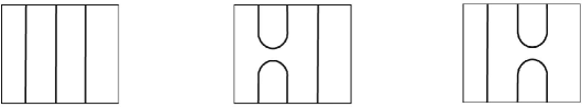
Figure 1. Generators of $TL_{3}$

A nice feature of this representation is that requiring that the $e_{i}$ satisfy the TL algebra imposes “$d$-isotopy”, cf [14]. Namely, a circle (simple closed curve) can be removed by multiplying the corresponding element in $TL$ by $d$. All isotopic pictures (which can be deformed continuously into each other without lines crossing and while keeping the points on the boundary fixed) are considered equivalent.

Various presentations of the TL algebra can be used to define lattice statistical-mechanical models. When the $e_{i}$ are represented by matrices, the degrees of freedom are usually referred to as spins or heights. For example, in the $Q$-state Potts model, the degrees of freedom are “spin” variables $\sigma_{i}$ taking integer values $1\dots Q$ at each site of some lattice. The $e_{i}$ here are represented by tensor products of $Q\times Q$ matrices, with $d=\sqrt{Q}$. The transfer matrix of the $Q$-state Potts model, with $n$ the number of sites on a zig-zag line, can be written entirely in terms of these generators. At the isotropic self-dual point for $n$ even, this transfer matrix for the square lattice is

(2.2) $$T=\left[\prod_{j=1}^{n/2}(1+e_{2j})\right]\left[\prod_{j=1}^{n/2}(1+e_{2j-1})\right]$$

The partition function for an $n\times m$ system with periodic boundary conditions in the $m$ direction is then $Z=\hbox{tr}\,T^{m}$.

A closely related way of defining a statistical mechanical model is via a pictorial presentation. For this presentation of the TL algebra, this results in the completely packed loop model. This model is defined on any graph with four edges per vertex. Each edge of the graph is covered by a loop, and at each vertex the loops avoid each other in the two possible ways. By using the pictures in figure 1, each configuration then corresponds to a single word in the TL algebra (i.e. some product of the $e_{i}$). The transfer matrix on the square lattice at the self-dual point remains (2.2); each factor $(1+e_{i})$ describes the two choices for the loops’ behavior at a single vertex. Expanding the product in $T^{m}$ into individual words corresponds to writing the partition function as a sum over loop configurations. The Boltzmann weight of each configuration in the completely packed loop model is the “evaluation” or the “Markov trace” of the corresponding element. This is a linear map of the algebra to the complex numbers, namely, the trace $tr_{d}\colon\thinspace TL^{d}_{n}\longrightarrow{\mathbb{C}}$ is defined on the additive generators (rectangular pictures) by connecting the top and bottom endpoints by disjoint arcs in the complement of the rectangle $R$ in the plane. The result is a disjoint collection of circles in the plane, which are then evaluated by taking $d^{\#circles}$. This completely packed loop model is still often referred to as the Potts model in its “Fortuin-Kasteleyn” or “cluster” representation [13]. Note however that although the Potts model is originally defined with $Q=d^{2}$ an integer, in this representation of the TL algebra this constraint is no longer required.

Utilizing this pictorial representation and the Markov trace allows one to relate the Jones polynomial of knot theory to the TL algebra [19]. Namely, the Jones polynomial can then be computed by projecting a knot or a link onto the plane, where in non-trivial cases the projection will include overcrossings and undercrossings. These are described by another geometric realization of $TL_{n}$. Here the elements are framed tangles in $D^{2}\times[0,1]$ which meet the top and the bottom of the cylinder in $n$ specified points, modulo the isotopy and the skein relations

(2.3) $$\slashoverback\;=\;\;A\;\smoothing\;+\;A^{-1}\;\hsmoothing\qquad{\rm and}\qquad{\mathcal{L}}\;\cup\bigcirc\;=\;(-A^{2}-A^{-2})\;{\mathcal{L}}\ .$$

We call this the skein-theoretic version, $TL_{n}^{\rm skein}$, while the planar one discussed above is $TL_{n}^{\rm planar}$. The planar approach is more suitable for applications to $2D$ lattice models, while skein theory provides a more well-known route to the construction of topological quantum field theories. However, it is easy to see that if we set $d=-A^{2}-A^{-2}$, one has the isomorphisms $TL_{n}\cong TL_{n}^{\rm skein}\cong TL_{n}^{\rm planar}$, and we use the superscript only to indicate a specific geometric context.

Up to overall factors of $A$, the Jones polynomial for a given collection of links is the Markov trace of the corresponding element of the algebra. Precisely, the trace $tr_{\langle\rangle}\colon\thinspace TL_{n}^{\rm skein}\longrightarrow{\mathbb{C}}$ is defined on the generators (framed tangles) by connecting the top and bottom endpoints by standard arcs in the complement of $D^{2}\times[0,1]$ in $3$-space, sweeping from top to bottom, and computing the Kauffman bracket [19]. (The Kauffman bracket $\langle L\rangle$ of a link $L$ in $S^{3}$ is defined by the skein relations (2.3).) It follows from these definitions that the two traces on $TL_{n}$ are equal up to the change of basis, in other words the diagram

(2.4)

commutes. The isomorphism above is given by viewing the generators of $TL_{n}^{\rm planar}$ as elements in $TL_{n}^{\rm skein}$ by including the rectangle $R$ as a vertical slice of the cylinder $D^{2}\times[0,1]$. The inverse map $TL_{n}^{\rm skein}\longrightarrow TL_{n}^{\rm planar}$ is defined by resolving any tangle, using the skein relation (2.3), into a linear combination of embedded planar pictures.

The relation of the foregoing to topological field theory is well known: the Jones polynomial of a collection of links correspond to a correlation function of Wilson loops in $SU(2)$ Chern-Simons gauge theory [37, 36]. These Wilson loops transform in the spin-1/2 representation of the $SU(2)$ algebra. Since the spin $1/2$ representation of $SU(2)$ is the simplest non-trivial representation of the simplest non-abelian Lie algebra, it is natural to expect that the previous results have a myriad of generalizations.

3. The chromatic algebra

The purpose of this section is to define the “chromatic algebra”. It is studied in further detail in section 4, and in sections 5, 6 the chromatic algebra is related to the $SO(3)$ BMW algebra.

The chromatic polynomial ${\chi}_{\Gamma}(Q)$ of a graph $\Gamma$, for $Q\in{\mathbb{Z}}_{+}$, is the number of colorings of the vertices of $\Gamma$ with the colors $1,\ldots,Q$ where no two adjacent vertices have the same color. To study ${\chi}_{\Gamma}(Q)$ for non-integer values of $Q$, it is often convenient to utilize the contraction-deletion relation (cf [2]). Given any edge $e$ of $\Gamma$ which is not a loop,

(3.1) $$\chi_{\Gamma}(Q)={\chi}_{{\Gamma}\backslash e}(Q)-{\chi}_{{\Gamma}/e}(Q)$$

where ${\Gamma}\backslash e$ is the graph obtained from $\Gamma$ by deleting $e$, and ${\Gamma}/e$ is obtained from $\Gamma$ by contracting $e$. (If $\Gamma$ contains a loop then ${\chi}_{\Gamma}\equiv 0$.) A useful consequence of the contraction-deletion relation is that

(3.2) $${\chi}_{\Gamma}(Q)=\sum_{S\subset\{{\rm edges\;\,of}\;\,{\Gamma}\}}(-1)^{|S|}\,Q^{k(S)}$$

where $k(S)$ is the number of connected components of the graph which has the same vertices as ${\Gamma}$ and whose edge set is given by $S$. Either of these two equations, together with the value on the graph consisting of a single vertex and no edges: ${\chi}(\cdot)=Q$ determines the chromatic polynomial, and may be used to define it for any (not necessarily integer) value of $Q$.

In section 2 we described how the completely packed loop model is related to (and can be defined using) the Temperley-Lieb algebra. To motivate what follows, it is useful to describe the analogous lattice statistical-mechanical model here. Remarkably, this model is also closely related to the Potts model, just like the completely packed loops. Instead of the FK/cluster expansion, the geometric degrees of freedom of interest here arise in the low-temperature expansion.

Each configuration of the Potts model is given by specifying the value $\sigma_{i}=1\dots Q$ of a spin at each vertex of some graph $L$ (which in physics applications is typically a lattice, but need not be). The Boltzmann weight of each configuration is then $e^{-\beta{\mathcal{E}}}$, where $\beta$ is inverse temperature, and the energy is

(3.3) $${\mathcal{E}}=-J\sum_{<ij>}\delta_{\sigma_{i}\sigma_{j}}$$

for nearest-neighbor sites labeled by $i$ and $j$. $J$ is a coupling, so that when $J>0$ the model is ferromagnetic, and when $J<0$ it is antiferromagnetic. The partition function is then defined as

(3.4) $$Z=\sum_{\{\sigma_{i}=1,\dots,Q\}}e^{-\beta{\mathcal{E}}}$$

where the sum is over all configurations.

To understand the low-temperature expansion, it is useful to first describe the zero-temperature antiferromagnetic limit, where $\beta\to\infty$ and $J<0$. The only configurations which contribute to the sum for $Z$ in (3.4) in this limit are those in which adjacent spins have different values. $Z$ then simply counts the number of such configurations, because each has the same weight $1$. Thus when $J<0$,

$$\lim_{\beta\to\infty}Z=\chi_{L}(Q)\ .$$

Thus the chromatic polynomial arises very naturally in statistical mechanics.

The low-temperature expansion is an expansion of $Z$ in powers of $e^{\beta J}$. It is useful intuitively to describe this in terms of domain walls on the dual graph $\widehat{L}$. Given $G\in{\mathcal{G}}$, the vertices of its dual graph $\widehat{G}$ correspond to the complementary regions $R\smallsetminus G$, and two vertices are joined by an edge in $\widehat{G}$ if and only if the corresponding regions share an edge, as shown in figure 2.

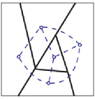
Figure 2. An element $G$ of ${\mathcal{G}}_{2}$ and its dual graph $\widehat{G}$ (drawn dashed).

With each configuration of spins, one associates a subgraph $N$ of $\widehat{L}$ by the following rule: when the spins on two sites differ, then the edge separating them belongs to $N$. If the spins are the same, the corresponding edge is not part of $N$. The graph $N$ is a domain-wall configuration, separating domains of like spins from each other. By construction, a domain-wall configuration $N$ consists of a graph with no ends (no 1-valent vertices) except possibly at the outside of $L$. For this reason we call such graphs “nets”. In the zero-temperature limit, all spin configurations contributing to the sum in $Z$ are associated to a single net $N=\widehat{L}$.

The idea of the low-temperature expansion is to first find the domain-wall configuration $N$ associated to a given spin configuration. Typically, many spin configurations are associated to the same $N$. By construction, the number of these is precisely the chromatic polynomial $\chi_{\widehat{N}}(Q)$. Each of these has the same Boltzmann weight $e^{\beta J(E(\widehat{L})-E(N))}$, where $E(G)$ is the number of edges in the graph $G$. $E(N)$ can be thought of as the “length” of the domain walls. The partition function is then

(3.5) $$Z=e^{\beta JE(\widehat{L})}\sum_{N}e^{-\beta JE(N)}\chi_{\hat{N}}(Q)$$

where the sum is over all subgraphs $N$ of $\widehat{L}$. (Here we can ignore the restriction that $N$ have no 1-valent vertices because $\chi_{\widehat{G}}(Q)=0$ for any graph $G$ with 1-valent vertices.) This shows that the $Q$-state Potts model has a very natural description as a sum over geometric objects, nets. Note also that this allows the model defined for any $Q$.

In section 2, we explained how the partition function of the completely packed loop model is defined as a sum over geometric objects, with each configuration associated with an element of the Temperley-Lieb algebra. It is thus natural to define an algebra whose elements correspond to nets, and whose Markov trace gives the chromatic polynomial. We therefore define the chromatic algebra in the same fashion as the TL defined in section 2. Consider the set ${\mathcal{G}}_{n}$ of the isotopy classes of planar graphs $G$ embedded in the rectangle $R$ with $n$ endpoints at the top and $n$ endpoints at the bottom of the rectangle. The intersection of $G$ with the boundary of $R$ consists precisely of these $2n$ points. In the Potts model, a graph $G$ is comprised of the domain walls separating regions of like spins from each other. It is convenient to divide the set of edges of $G$ into outer edges, i.e. those edges that have an endpoint on the boundary of $R$, and inner edges, whose vertices are in the interior of $R$. (Note that the graphs $G$ are not necessarily connected.) It is convenient to allow $G$ to have connected components which are simple closed curves (which are not strictly speaking “graphs” since they do not contain a vertex.)

Notation 3.1.

While discussing the chromatic algebra, we will interchangeably use two variables, $Q$ and $q$. Set $Q=q+2+q^{-1}=(q^{1/2}+q^{-1/2})^{2}$.

The defining contraction-deletion rule (3.1) may be viewed as a linear relation between the graphs $G,G/e$ and $G\backslash e$, so in this context it is natural to consider the vector space defined by graphs, rather than just the set of graphs. Thus let ${\mathcal{F}}_{n}$ denote the free algebra over ${\mathbb{C}}[Q]$ with free additive generators given by the elements of ${\mathcal{G}}_{n}$. As usual, the multiplication is given by vertical stacking, and we set ${\mathcal{F}}=\cup_{n}{\mathcal{F}}_{n}$.

The local relations among the elements of ${\mathcal{G}}_{n}$, analogous to contraction-deletion rule for the chromatic polynomial, are given in figures 3, 4. Note that these relations only apply to inner edges which do not connect to the top and the bottom of the rectangle. They are

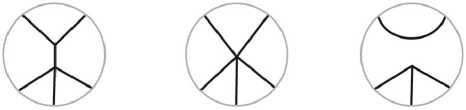
Figure 3. Relation (1) in the chromatic algebra

(1) If $e$ is an inner edge of a graph $G$ which is not a loop, then $G=G/e-G\backslash e$, figure 3.

(2) If $G$ contains an inner edge $e$ which is a loop, then $G=(Q-1)\;G\backslash e$, figure 4. (In particular, this relation applies if $e$ is a simple closed curve not connected to the rest of the graph.)

(3) If $G$ contains a $1$-valent vertex (in the interior of the rectangle) then $G=0$, figure 4.

Figure 4. Relations (2), (3) in the chromatic algebra

Definition 3.2.

The chromatic algebra in degree $n$, ${\mathcal{C}}_{n}$, is an algebra over ${\mathbb{C}}[Q]$ which is defined as the quotient of the free algebra ${\mathcal{F}}_{n}$ by the ideal $I_{n}$ generated by the relations (1), (2), (3). Set ${\mathcal{C}}=\cup_{n}{\mathcal{C}}_{n}$.

The ideal $I_{n}$ in the definition above is generated by linear combinations of graphs in ${\mathcal{F}}_{n}$ which are identical outside a disk embedded in the rectangle, and which differ according to one of the relations $(1)-(3)$ in the disk.

Remark 3.3.

Recall that $e$ is a bridge if it is an internal edge which, if removed, disconnects $G$ (considering all points on the boundary of $R$ to be connected). The relation (3) above can be replaced by

(3^′): If $G$ has a bridge $e$ then $G=0$.

Note that this means the dual graph $\widehat{G}$ contains a loop.

We will now collect some elementary consequences of the relations which hold in ${\mathcal{C}}$: (1) and (3) imply that a $2$-valent vertex may be deleted, and the two adjacent edges merged, figure 5 (the dual graph, discussed in more detail below, is drawn dashed.) (1) and (3) also imply that if a graph $G$ contains an isolated vertex $v$, then $G=G\backslash v$. (Note that deleting an isolated vertex does not change the dual graph.) Figure 6 gives more examples of relations which hold in ${\mathcal{C}}_{2}$. It is important to note that the relations (1) – (3) are consistent with the relations for the chromatic polynomial of the dual graph, see the following proposition.

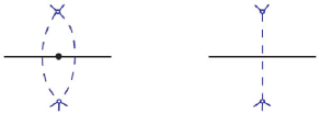
Figure 5.

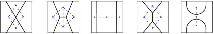
Figure 6.

Proposition 3.4.

The chromatic polynomial gives rise to a well-defined linear map ${\chi}\colon\thinspace{\mathcal{C}}_{n}\longrightarrow{\mathbb{C}}[Q]$. This map is defined on the additive generators $G$ as the chromatic polynomial of the dual graph, ${\chi}_{\widehat{G}}$, and it is extended to ${\mathcal{C}}_{n}$ by linearity.

To prove this proposition, one needs to check that the relations (1)-(3) hold when one considers the chromatic polynomial of the dual graph. Specifically, in case (1) consider the edge $\hat{e}$ of $\widehat{G}$, dual to $e$, figure 7. Then $\widehat{G/e}=\widehat{G}\backslash\hat{e}$, and $\widehat{G\backslash e}=\widehat{G}/\hat{e}$. (In the case when one of the vertices of $e$ is trivalent, as in figure 7, $\widehat{G}/\hat{e}$ differs from $\widehat{G\backslash e}$ by the addition of an edge parallel to $\hat{e}_{1}$, figure 7. Because of the equality in figure 5, ${\chi}_{\widehat{G}/\hat{e}}={\chi}_{\widehat{G\backslash e}}$ still holds in this case.) Therefore the relation (1) translates to ${\chi}_{\widehat{G}}={\chi}_{\widehat{G}\backslash\hat{e}}-{\chi}_{\widehat{G}/\hat{e}}$, the defining contraction-deletion relation for the chromatic polynomial.

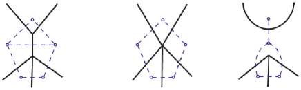
Figure 7. Relation (1) and the dual graphs

To check (2), note that if $G$ contains a loop which is trivial in the plane (i.e. the region $D$ bounded by it is disjoint from the graph), the dual graph $\widehat{G}$ contains a $1$-valent vertex (corresponding to the region $D$.) The effect of deleting such a vertex and the adjacent edge on the chromatic polynomial ${\chi}_{\widehat{G}}(Q)$ is multiplication by $(Q-1)$. The general case when the region $D$ bounded by the loop contains other vertices or edges of $G$ follows by applying (1) and (3) to the part of the graph inside $D$, and then inductively applying the case of (2) considered above to the trivial inner-most loops of $G$.

The relation (3) holds since in this case the dual graph has a loop, therefore its chromatic polynomial vanishes. ∎

Definition 3.5.

The trace, $tr_{\chi}\colon\thinspace{\mathcal{C}}\longrightarrow{\mathbb{C}}$ is defined on the additive generators (graphs $G$ in the rectangle $R$) by connecting the top and bottom endpoints of $G$ by disjoint arcs in complement of $R$ the plane (denote the result by $\overline{G}$) and evaluating the chromatic polynomial of the dual graph:

(3.6) $$tr_{\chi}(G)\;\,=\;\,Q^{-1}\cdot{\chi}_{\widehat{\overline{G}}}(Q).$$

Proposition 3.4 shows that the trace is well defined. The factor $Q^{-1}$ is a convenient normalization which makes the relation with the BMW algebra easier to state (see sections 5, 6); with this normalization, $tr_{\chi}(\cdot)=1$. The Hermitian product on ${\mathcal{C}}_{n}$ is defined analogously to the Temperley-Lieb case: $\langle a,b\rangle=\hbox{tr}(a\,\bar{b})$, where the involution $\bar{b}$ is defined by conjugating the complex coefficients, and on an additive generator $b$ (a graph in $R$) it is defined as the reflection in a horizontal line, see figure 8.

Figure 8. The inner product in ${\mathcal{C}}_{3}$: $Tr(a\,\overline{b})$ equals the evaluation of $\overline{G}$, or equivalently $Q^{-1}$ times the chromatic polynomial of the dual graph $\widehat{\overline{G}}$. In this example, $\overline{G}$ is the theta graph, and

$$\langle a,b\rangle\,=\,Q^{-1}\cdot(Q(Q-1)(Q-2))=(Q-1)(Q-2).$$

Remark 3.6.

The chromatic polynomial ${\chi}_{G}$ and the Potts-model partition (3.5) function are specializations of the more general Tutte polynomial $T_{G}(X,Y)$, cf [2]. The Tutte polynomial satisfies the well-known duality $T_{G}(X,Y)=T_{\widehat{G}}(Y,X)$, where $G$ is a planar graph and $\widehat{G}$ is its dual. Therefore, rather then defining the trace of the chromatic algebra as the chromatic polynomial of the dual graph $\widehat{G}$, one could define the trace as the corresponding relevant specialization of the Tutte polynomial (sometimes known as the flow polynomial) of the graph $G$ itself.

Remark 3.7.

One could generalize the definition of ${\mathcal{C}}$ and consider the “Tutte algebra” whose trace is given by the Tutte polynomial. We restrict our discussion to the special case of the chromatic polynomial since it corresponds to our main object of interest, the $SO(3)$ BMW algebra, see sections 5, 6. Another reason for this is that the chromatic algebra gives rise to the $(2+1)$-dimensional $SO(3)$ TQFT (see section 3.1), and this seems to be the only specialization of the Tutte polynomial which yields a finite dimensional unitary TQFT.

3.1. From algebras to TQFTs

There is a well-understood route for representing $(2+1)-$ dimensional topological quantum field theories in terms of “pictures” on surfaces modulo local relations, see [36], [15]. This is described in depth in the case of (doubled) $SU(2)$ theories in [14]. Here we briefly sketch the analogous construction of the doubled (Turaev-Viro [31]) $SO(3)$ TQFTs (developed in [27], [30].) In fact, the problem of finding a description of these TQFTs in terms of ($2-$dimensional) pictures and relations was a starting point for our introduction of the chromatic algebra in this paper. The description of TQFTs in such terms is important for applications in physics, specifically to lattice models exhibiting topological order [14], [24].

Given a compact surface ${\Sigma}$, consider the (infinite-dimensional) complex vector space $V_{1}$ consisting of formal linear combinations of the isotopy classes of graphs embedded in $\Sigma$. If $\Sigma$ has a non-empty boundary, one fixes a boundary condition – a finite number of points in the boundary $\partial\Sigma$, and the graphs in $\Sigma$ should meet the boundary in these specified points. Consider the quotient $V_{2}^{Q}$ of $V_{1}$ by the local relations $(1)$-$(3)$ defining the chromatic algebra as in 3.2. Equivalently, one may start with the space of trivalent graphs, modulo the relations in figure 9, see theorem 4.3 in the next section. The chromatic algebra ${\mathcal{C}}^{Q}$ (more precisely, its generalization, the chromatic category, see section 4 in [10]) is a local version of $V_{2}^{Q}$, i.e. it corresponds to ${\Sigma}=$disk.

The vector space $V_{2}^{Q}$ is still infinite-dimensional. However, at the special values of $Q$ known as Beraha numbers, $Q=B_{n}=2+2\cos(2{\pi}/n)$, there are additional local linear relations such that the quotient, $V^{\Sigma}_{n}$, is finite dimensional. These additional local relations are generators of the trace radical of the chromatic algebra, i.e. elements $a$ of ${\mathcal{C}}^{B_{n}}$ such that $\langle a,b\rangle=Tr(a\bar{b})=0$ for all $b\in{\mathcal{C}}^{B_{n}}$. The trace pairing descends to a positive-definite Hermitian product on the quotient of ${\mathcal{C}}^{B_{n}}$ by the trace radical (see corollary 7.2), which gives rise to a positive-definite Hermitian product on $V^{\Sigma}_{n}$, see [36]. (The trace radical is analyzed in [10], where we show that it contains the pull-back of the Jones Wenzl-projector from the Temperley-Lieb algebra, and give applications of this fact to the structure of the chromatic polynomial of planar graphs.)

These finite-dimensional vector spaces, $V^{\Sigma}_{n}$, are the doubled $SO(3)$ TQFTs, and the unitary structure on these TQFTs is induced by the trace pairing on the chromatic algebra as indicated above. The structure of the simplest non-trivial TQFT which arises from this construction, corresponding to $Q=B_{5}={\phi}+1$, and which is known as the “doubled Fibonacci theory”, is considered in [12]. In this paper we analyze some of the algebraic structure underlying these TQFTs for other levels $n$.

4. A trivalent presentation of the chromatic algebra

In this section we define an algebra using trivalent graphs modulo certain simple relations consistent with the contraction-deletion rule, and prove that it is isomorphic to the chromatic algebra. This result should be compared with section 5 which shows that, in contrast, a presentation of this algebra in terms of four-valent graphs is rather involved. As part of the proof, in this section we find an additive basis of the chromatic algebra ${\mathcal{C}}_{n}$ in terms of planar partitions, and we establish an algebra analogue of the “state sum” formula (3.2) for the chromatic polynomial. Both the chromatic algebra and its trivalent presentation established here are used in our companion paper [10] to prove and generalize Tutte’s identities for the chromatic polynomial.

Definition 4.1.

Analogously to definition 3.2, consider the free algebra ${\mathcal{FT}}_{n}$ over ${\mathbb{C}}[Q]$ whose elements are formal linear combinations of the isotopy classes of trivalent graphs in a rectangle $R$. The intersection of each such graph with the boundary of $R$ consists of precisely $2n$ points: $n$ points at the top and the bottom each. Let ${\mathcal{T}}_{n}$ denote the quotient of ${\mathcal{FT}}_{n}$ by the ideal generated by the local relations shown in figure 9.

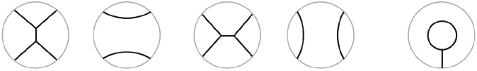
Figure 9. Trivalent presentation of the chromatic algebra.

Remark 4.2.

Note that the vertices of the graphs in the definition above in the interior of $R$ are trivalent, in particular they do not have ends ($1$-valent vertices) other than those on the boundary of $R$. It is convenient to allow $2$-valent vertices as well, so there may be loops disjoint from the rest of the graph.

The relations in ${\mathcal{T}}$, shown in figure 9, have a rather natural interpretation in the context of TQFTs discussed in section 3.1. The second relation says that the vector space associated to the disk with a single boundary label is trivial. The first relation implies that the vector space associated to the disk with four boundary labels is $3$-dimensional.

Theorem 4.3.

The map ${\Phi}\colon\thinspace{\mathcal{T}}_{n}\longrightarrow{\mathcal{C}}_{n}$, induced by the inclusion of the trivalent graphs in the set of all graphs, is an algebra isomorphism.

First observe that $\Phi$ is well-defined. Indeed, the first relation in figure 9 is a consequence of the contraction-deletion rule (1) in the definition of ${\mathcal{C}}_{n}$, see figure 6. The relation on the right in figure 9 is a consequence of relations (2), (3) defining ${\mathcal{C}}_{n}$. Moreover, $\Phi$ is a surjective map: using the contraction-deletion rule (1), any graph $G\in{\mathcal{G}}_{n}$ may be expressed as a linear combination of trivalent graphs. This establishes

(4.1) $$dim_{\mathbb{C}}({\mathcal{T}}_{n})\geq dim_{\mathbb{C}}({\mathcal{C}}_{n}).$$

We start the proof of the converse inequality by presenting an algebra analogue of the expansion (3.2) of the chromatic polynomial. This expansion is then used for describing a linearly independent set of additive generators of ${\mathcal{C}}_{n}$.

Following the terminology introduced in section 3, given a graph $G$ in the rectangle $R$, $G\in{\mathcal{G}}_{n}$, we consider its set of inner edges, the edges of $G$ whose endpoints are not on the boundary of $R$. Consider the set $B_{n}$ of all graphs in ${\mathcal{G}}_{n}$ without inner edges, as in figure 10. (Note that the elements of $B_{n}$ are in $1-1$ correspondence with the planar partitions of the set of $2n$ boundary vertices such that each block of the partition contains at least two vertices.)

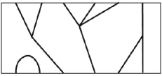
Figure 10. An example of a graph in $B_{6}$.

Lemma 4.4.

The elements of $B_{n}$ form an additive basis of the chromatic algebra ${\mathcal{C}}_{n}$.

Proof. Consider the vector space $V_{n}$ over ${\mathbb{C}}$ spanned by $B_{n}$. Define linear maps ${\phi}\colon\thinspace V_{n}\longrightarrow{\mathcal{C}}_{n}$ and ${\psi}\colon\thinspace{\mathcal{C}}_{n}\longrightarrow V_{n}$. Here ${\phi}$ is induced by the inclusion $B_{n}=\{$isotopy classes of graphs without inner edges in the rectangle $R\}\subset\{$isotopy classes of all graphs in $R\}={\mathcal{G}}_{n}$, while $\psi$ is defined using an expansion similar to the expansion (3.2) for the chromatic polynomial: for $G\in{\mathcal{G}}_{n}$, set

(4.2) $${\psi}(G)=\sum_{S\,\subset\,\{{\rm inner\;\,edges\;\,of}\;\,G\}}\;(-1)^{E(G)-|S|}\,\;Q^{n(S)}\;b_{S}\ ,$$

where $E(G)$ is the number of edges of the graph $G$ and $n(S)$ is the nullity of the graph $G_{S}$ which is obtained by keeping all vertices and outer edges of $G$ and adding just those inner edges which are in $S$. (Here the nullity is the number of independent cycles, i.e. the rank $rk(H_{1}(G_{S},{\mathbb{Z}}))$ of the first homology group of $G_{S}$.) In the formula above $b_{S}$ is the unique element of $B_{n}$ which gives rise to the same partition of the $2n$ boundary points as $G_{S}$, in other words $b_{S}$ is obtained from $G_{S}$ by contracting each of its inner edges.

The proof that ${\psi}$ is well-defined is analogous to the proof that the expansion (3.2) of the chromatic polynomial satisfies the contraction-deletion rule. Specifically, consider the relations $(1)-(3)$ defining the chromatic algebra (definition 3.2). For $(1)$, suppose $e$ is an inner edge which is not a loop. The sum (4.2) splits as the sum over the sets $S^{\prime}$ which contain the edge $e$ and the sets $S^{\prime\prime}$ which do not. The sets $S^{\prime}$ are in $1-1$ correspondence with the sets of edges of $G/e$; the correspondence is given by contracting $e$. Under this correspondence, the nullity is preserved, and each term in the sum over the sets $S^{\prime}$ is equal to the corresponding term in the sum for the graph $G/e$. Similarly, the sets $S^{\prime\prime}$ are in $1-1$ correspondence with the sets of edges of $G\smallsetminus e$, and the corresponding terms in the two sums differ in their sign. Therefore ${\psi}(G)={\psi}(G/e)-{\psi}(G\smallsetminus e)$, proving the invariance of ${\psi}$ under the relation $(1)$.

To establish the invariance under $(2)$, let $e$ be a loop in $G$. Again, (4.2) splits as the sum over the sets $S^{\prime}$ which contain $e$ and the sets $S^{\prime\prime}$ which do not. Both $S^{\prime}$ and $S^{\prime\prime}$ are in $1-1$ correspondence with the subsets of inner edges of $G\smallsetminus e$. Each term from $S^{\prime}$ with $e$ has an extra factor of $Q$ because $n(S^{\prime})=n(G\smallsetminus e)+1$, while each term from $S^{\prime\prime}$ has an extra factor of $(-1)$. Combining these, one gets ${\psi}(G)=(Q-1){\psi}(G\smallsetminus e)$. The invariance under $(3)$ is proved analogously: if $G$ contains a $1$-valent vertex, let $e$ be its adjacent edge. Dividing the subsets into $S^{\prime}$ and $S^{\prime\prime}$ as above, one checks that the corresponding terms cancel in pairs. This shows that $\psi$ is well-defined.

It follows from the contraction-deletion rule (1) that any graph may be expressed as a linear combination of graphs without inner edges (elements of $B_{n}$). Therefore the dimension of ${\mathcal{C}}_{n}$ is less than or equal to the cardinality of $|B_{n}|$. On the other hand, the composition $V_{n}\longrightarrow{\mathcal{C}}_{n}\longrightarrow V_{n}$ is an isomorphism (for $b\in B_{n}$, ${\psi}({\phi}(b))=\pm b$), proving the opposite inequality $|B_{n}|=dim(V_{n})\leq dim({\mathcal{C}}_{n})$. Therefore $dim(V_{n})=dim({\mathcal{C}}_{n})$ and $B_{n}$ is a basis of ${\mathcal{C}}_{n}$. This completes the proof of lemma 4.4. ∎

Remark 4.5.

The seeming difference between the expansions (3.2) and (4.2) is due to the definition of the chromatic algebra: its trace is the chromatic polynomial of the dual graph. The expansion (4.2) is directly analogous to the expansion for the flow polynomial, see remark 3.6. Indeed, the quantities $k(S)$ and $n(S)$ in the two expansions correspond to each other under the duality between $G$ and $\widehat{G}$.

With this result at hand, we will now proceed with the proof of theorem 4.3. For each element $\Gamma$ of $B_{n}$ pick a trivalent graph $T_{\Gamma}$ such that $H_{1}(T_{\Gamma})=0$ ($T_{\Gamma}$ is a disjoint union of trees) and the contraction of all inner edges of $T_{\Gamma}$ gives $\Gamma$. Let $TB_{n}$ denote the set of such trivalent graphs $\{T_{\Gamma},{\Gamma}\in B_{n}\}$; by construction $TB_{n}$ is in a bijective correspondence with $B_{n}$. It is useful for the following argument to note that the combinatorial F-move, exchanging the first and third trivalent graphs in figure 9 and applied at various inner edges of trivalent graphs, acts transitively on the set of all possible choices of the graphs $T_{\Gamma}$, for a given ${\Gamma}$.

We claim that any element of ${\mathcal{T}}_{n}$ is a linear combination of elements of $TB_{n}$. Indeed, given $T\in{\mathcal{T}}_{n}$, using the relations in figure 9 defining ${\mathcal{T}}_{n}$, $T$ is seen to be a linear combination of elements $T_{i}\in{\mathcal{T}}_{n}$ where each $T_{i}$ does not have cycles: $H_{1}(T_{i})=0$. Now contracting all inner edges of each $T_{i}$ gives rise to an element ${\Gamma}_{i}\in B_{n}$. As noted above, for each $i$ there is a sequence of $F$-moves taking $T_{i}$ to the corresponding $T_{{\Gamma}_{i}}\in TB_{n}$. Applying the linear relation on the left in figure 9 each time the $F$-move is needed shows that $T_{i}=T_{{\Gamma}_{i}}+$terms with fewer trivalent vertices. Now an inductive argument, where the induction is on the number of trivalent vertices, proves the claim that any element of ${\mathcal{T}}_{n}$ is a linear combination of elements of $TB_{n}$. Using lemma 4.2, this shows that

$$dim_{\mathbb{C}}{\mathcal{T}}_{n}\leq|TB_{n}|=|B_{n}|=dim_{\mathbb{C}}{\mathcal{C}}_{n}.$$

Combined with the inequality 4.1, this completes the proof of theorem 4.3. ∎

5. The chromatic algebra and the $SO(3)$ BMW algebra

In this section we find a homomorphism from the $SO(3)$ BMW algebra to the chromatic algebra, showing that the defining relations for $BMW(3)$ reduce to the contraction-deletion rule for planar graphs. Since the $SO(3)$ Kauffman polynomial arises from the Markov trace of the $SO(3)$ BMW algebra, this enables us to relate this link invariant to the chromatic polynomial, and so provide geometric intuition into the planar description of the algebra.

To give some intuition into why these two algebras are related, it is useful to recall some results for the integrable field theory describing the scaling limit of the $Q$-state Potts model near the critical point. A oft-useful description of an integrable two-dimensional classical field theory is in terms of the quasiparticles and their scattering matrices in the corresponding one-dimensional quantum field theory. For this Potts field theory, the scattering matrices are invariant under the quantum-group algebra $U_{q}(SO(3))$ when the quasiparticles transform in the spin-1 representation [28]. This implies that the scattering matrices can be written in terms of the generators of the $SO(3)$ BMW algebra. However, intuitive arguments suggest that the world lines of the quasiparticles should behave as domain walls separating regions of like spins [6]. These two very different pictures were reconciled in [11]. There it was shown how the generators of the $SO(3)$ BMW algebra subalgebra were those of the chromatic algebra containing only 4-valent vertices. This correspondence was exploited in [8] to study quantum loop models. Here we use this motivation to give an elegant combinatorial-geometric description of $BMW(3)$.

We start with a review of the background material on the $SO(N)$ Birman-Murakami-Wenzl algebra; see [4, 26] for more details. Here we present the $SO(N)$ BMW algebra in skein form. A strand can be thought of as corresponding to the fundamental (dimension $N$) representation of $U_{q}(SO(N))$. The braiding generators (the over/under crossings) are displayed in figure 11.

Figure 11. Braiding generators of $BMW(N)_{3}$.

As opposed to $TL$, the skein relations do not allow one to reduce all braids to non-crossing curves. Instead, $BMW(N)_{n}$ is the algebra of framed tangles on $n$ strands in $D^{2}\times[0,1]$ modulo isotopy and the $SO(N)$ Kauffman skein relations in figure 12.

Figure 12.

By a tangle we mean a collection of curves (some of them perhaps closed) embedded in $D^{2}\times[0,1]$, with precisely $2n$ endpoints, $n$ in $D^{2}\times\{0\}$ and $D^{2}\times\{1\}$ each, at the prescribed marked points in the disk. The tangles are framed, i.e. they are given with a trivialization of their normal bundle. (This is necessary since the last two relations in figure 12 are not invariant under the first Reidemeister move.) As with $TL$, the multiplication is given by vertical stacking. Like above, $BMW(N)=\cup_{n}BMW(N)_{n}$.

We now turn to a presentation of this algebra: the generators of $BMW(N)_{n}$ include the Temperley-Lieb generators $1,\,e_{1},\ldots,e_{n-1}$ as above, and additionally the braiding generators $B_{i},\,B^{-1}_{i}$, $i=1,\ldots,n-1$, figure 11. (This follows by considering the height Morse function.) In the algebraic context, the relations in $BMW_{n}$ are the Temperley-Lieb relations (2.1) and in addition

(5.1) $$B_{i}e_{i}=q^{1-N}e_{i},\qquad B_{i}e_{i-1}^{\pm 1}B_{i}=q^{\pm(N-1)}B_{i},\qquad B_{i}-B_{i}^{-1}=(q-q^{-1})(1-e_{i}).$$

We will usually work with the geometric counterparts of these relations: isotopy (expressed as Reidemeister moves for framed tangles), and the skein relations in figure 12.

Sending the generators of $TL_{n}$ to the corresponding generators $e_{i}$ of $BMW(N)_{n}$ defines a map of algebras, and the skein relations require that deleting a circle has the effect of multiplying the element of $BMW(N)$ by

(5.2) $$d_{N}=1+\frac{q^{N-1}-q^{-(N-1)}}{q-q^{-1}}.$$

This gives for example $d_{3}=q+1+q^{-1}$ and $d_{4}=(q+q^{-1})^{2}$.

The trace, $\hbox{tr}_{K}\colon\thinspace BMW(N)_{n}\longrightarrow{\mathbb{C}}$, is defined similarly to the TL case. It is defined on the generators (framed tangles) by connecting the top and bottom endpoints by standard arcs in the complement of $D^{2}\times[0,1]$ in $3$-space, sweeping from top to bottom, and computing the $SO(N)$ Kauffman polynomial (given by the skein relations above) of the resulting link. Below we will discuss this trace in detail.

As with the Temperley-Lieb algebra, it is convenient to distinguish the skein-theoretic and planar presentations of this algebra, $BMW(N)^{\rm skein}$ and $BMW(N)^{\rm planar}$. In the planar version the additive generators are linear combinations of curves with crossings, or in other words $4$-valent graphs, in a rectangle. In terms of generators, the elements $B,B^{-1}\in BMW^{\rm skein}$ are replaced with $\crossing\in BMW(N)^{\rm planar}$, defined by [20]

(5.3) $$(\crossing)\;=\;q(\smoothing)-(\slashoverback)+q^{-1}(\hsmoothing)\;=\;q^{-1}(\smoothing)-(\backoverslash)+q(\hsmoothing).$$

$BMW(N)^{\rm planar}$ is defined as linear combinations of $4$-valent graphs in a rectangle modulo local relations which are the pull-back of (5.1) (or equivalently of the Kauffman skein relations and the isotopy of tangles) via (5.3). The equation (5.3) yields an isomorphism between the planar and skein presentations. We will discuss the relations in $BMW^{\rm planar}$ in more detail below.

The translation of the BMW relations 5.1 (geometrically seen as the skein relations and the isotopy of tangles) to the planar setting formally follows from the isomorphism (5.3). However, the geometric meaning of the planar description is not immediately apparent. The results of this paper provide such a meaning for $BMW(3)$. For the rest of the paper, we will omit the label and denote this algebra by $BMW$.

One easily checks that there is a map of algebras $TL_{n}\longrightarrow{\mathcal{C}}_{n}$, where the relation between the Temperley-Lieb and chromatic parameters is given by $d=Q-1=q+1+q^{-1}$. This map is induced by the inclusion $\{$curves$\}\subset\{$graphs$\}$ in a rectangle $R$. The defining relations for $TL_{n}$ ($d$-isotopy) hold in ${\mathcal{C}}_{n}$ due to the relation (2) in definition 3.2 of the chromatic algebra. The following statement shows that this map extends to $BMW_{n}$.

Theorem 5.1.

The formulas

(5.4) $$(\slashoverback)\,\mapsto\,q(\smoothing)-(\crossing)+q^{-1}(\hsmoothing),\;\;\;(\backoverslash)\,\mapsto\,q^{-1}(\smoothing)-(\crossing)+q(\hsmoothing)$$

define a homomorphism of algebras $i\colon\thinspace BMW^{\rm skein}_{n}\longrightarrow{\mathcal{C}}_{n}$ over ${\mathbb{C}}[q]$.

Remark 5.2.

It follows from theorem 6.3 below that the homomorphism $i$ preserves the traces of these algebras, see corollary 6.5.

Remark 5.3.

Abusing the notation, we will keep the same symbol for the map $i\colon\thinspace BMW^{\rm planar}_{n}\longrightarrow{\mathcal{C}}_{n}$. This homomorphism is induced by the inclusion $\{4$-valent graphs$\}\subset\{$all graphs$\}$. Recall that the relations in $BMW^{\rm planar}_{n}$ are the pullback of (5.1) under the identification (5.3), and the content of the theorem above is that these relations are a consequence of the contraction-deletion rule.

Remark 5.4.

The homomorphism $i$ is not surjective (one may check that for example, the graph in figure 13 is not equivalent in ${\mathcal{C}}_{3}$ to a linear combination of $4$-valent graphs), however it seems reasonable to conjecture that it is injective, in other words that $BMW_{n}$ is a subalgebra of the chromatic algebra ${\mathcal{C}}_{n}$ generated by $4$-valent graphs. Note that the chromatic algebra ${\mathcal{C}}_{n}$ has quite elegant presentations in terms of the contraction-deletion rule (definition 3.2), and in terms of trivalent graphs (definition 4.1). In contrast, the corresponding presentation in terms of $4$-valent graphs is rather involved: the relations are the pullback of (5.1) under the identification (5.3). See also a related discussion in section 8.3.

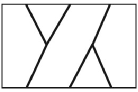
Figure 13.

Proof of theorem 5.1. One needs to show that the map $i$ is well-defined. The first defining relation of the BMW algebra (figure 12)

$$(\slashoverback)-(\backoverslash)\,=\,(q-q^{-1})[(\smoothing)-(\hsmoothing)]$$

follows directly from the equations (5.4). One needs to check that the last two relations in figure 12, as well as the regular isotopy of tangle diagrams (the second and third Reidemeister moves), hold in the chromatic algebra. The proof of the first of these is shown in figure 14.

Figure 14.

The last relation in figure 12 is established analogously. To prove the second Reidemeister move, start with the diagram on the left in figure 15 and resolve the crossings according to the formulas (5.4). Applying the contraction-deletion rule (1) in definition 3.2 of the chromatic algebra to the edges connecting the double points in the third term, eliminating the trivial circle in the last term according to the rule (2), and canceling the resulting terms, one gets the diagram on the right.

Figure 15.

The remaining relation is the third Reidemeister move: one has to show that the images of the two diagrams in figure 16 are equal in the chromatic algebra. Note that these two diagrams differ by a 180 degree rotation, so whenever a planar diagram, invariant under such a rotation, appears in the expansion of one of them, it also appears (with the same coefficient) in the expansion of the other one. Expanding the lower crossing of the diagram on the left according to (5.4), one gets the expression in figure 17.

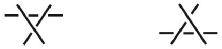
Figure 16.

It follows from the remark above, and from the proof of the second Reidemeister move that the first and the third terms in figure 17 cancel with the corresponding terms in the expansion of the second diagram in figure 16. Therefore it remains to show that the second term on the right in figure 17 equals its 180 degree rotation in the chromatic algebra.

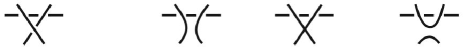
Figure 17.

Figure 18.

The expansion of this term according to (5.4) is shown in figure 18. The 4th and 8th terms are invariant under the 180 rotation. Omitting these two terms, and using the relations (1), (2) in the chromatic algebra to expand the terms with more than one double point, one gets the expression in figure 19.

Figure 19.

This expression is again invariant under a 180 degree rotation, and this concludes the proof for the third Reidemeister move and the proof of theorem 5.1. ∎

6. Relations between $TL$, $BMW$, and the chromatic algebra

In this section we investigate the relations between the $SO(3)$ Birman-Murakami-Wenzl, chromatic, and Temperley-Lieb algebras. The main result is stated in theorem 6.3. This relationship is useful in a variety of contexts. For example, it allows one to use the Jones-Wenzl projectors in $TL^{d}$, at special values of $d$, to analyze the structure of the trace radical of the BMW and chromatic algebras. This was used in [10] to find linear relations obeyed by the chromatic polynomial of planar graphs, evaluated at Beraha numbers. This also provides a relationship between certain string-net models and loop models, cf [12], [7]. Applying traces to these algebras, we express the $SO(3)$ Kauffman polynomial in terms of the chromatic polynomial, see corollary 6.5.

The $SO(3)$ BMW algebra may be described in several ways. First we explain how each strand of the BMW algebra may be viewed as a “fusion” of two Temperley-Lieb strands, in other words defining a homomorphism of the $SO(3)$ BMW algebra in degree $n$, $BMW_{n}$ to $TL_{2n}$. This description is particularly natural when studying quantum-group algebras, where each strand in $TL$ and $BMW$ correspond respectively to a spin-1/2 and spin-1 representation of $U_{q}(sl_{2})$.

In fact, we define a homomorphism from the chromatic algebra ${\mathcal{C}}_{n}\longrightarrow TL_{2n}$ which yields a map from the BMW algebra by pre-composing it with the homomorphism $i\colon\thinspace BMW_{n}\longrightarrow{\mathcal{C}}_{n}$, constructed in the previous section. Recall that the chromatic algebra ${\mathcal{C}}_{n}$ is defined as the quotient of the free algebra ${\mathcal{F}}_{n}$ by the ideal generated by the relations $(1)-(3)$ in definition 3.2.

Definition 6.1.

Define a homomorphism ${\phi}\colon\thinspace{\mathcal{F}}_{n}\longrightarrow TL_{2n}$ on the additive generators (graphs in a rectangle) of the free graph algebra ${\mathcal{F}}_{n}$ by replacing each edge with the linear combination ${\phi}(\;|\;)=\smoothing-\frac{1}{d}\,\hsmoothing\,$, and resolving each vertex as shown in figure 20. The factor in the definition of ${\phi}$ corresponding to a $r$-valent vertex is $d^{(r-2)/2}$, so for example it equals $d$ for the $4$-valent vertex in figure 20. The overall factor for a graph $G$ is the product of the factors $d^{(r(V)-2)/2}$ over all vertices $V$ of $G$.

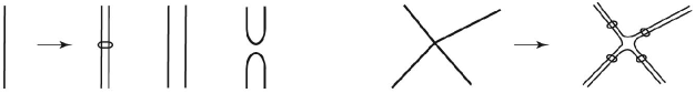
Figure 20. Definition of the homomorphism ${\phi}\colon\thinspace{\mathcal{C}}^{Q}_{n}\longrightarrow TL^{d}_{2n}$, where $Q=d^{2}$.

Therefore ${\phi}(G)$ is a sum of $2^{E(G)}$ terms, where $E(G)$ is the number of edges of $G$. Note that ${\phi}$ replaces each edge with the second Jones-Wenzl projector $P_{2}$, well-known in the study of the Temperley-Lieb algebra [17]. They are idempotents: $P_{2}\circ P_{2}=P_{2}$, and this identity (used in the definition of the homomorphism $\phi$) may be easily checked directly, figure 21.

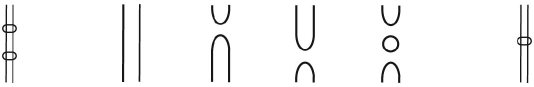
Figure 21. $P_{2}\circ P_{2}=P_{2}$

Various authors have considered versions of the map ${\phi}$ in the knot-theoretic and TQFT contexts, see [39, 16, 19, 12, 35]. In [11] this was used to give a map of the SO(3) BMW algebra to the Temperley-Lieb algebra.

Lemma 6.2.

${\phi}$ induces a well-defined homomorphism of algebras ${\mathcal{C}}^{Q}_{n}\longrightarrow TL^{d}_{2n}$, where $Q=d^{2}$.

Proof. One needs to check that ${\phi}$ is well-defined with respect to the relations $(1)-(3)$ in the chromatic algebra (definition 3.2). To establish (1), one applies ${\phi}$ to both sides and expands the projector at the edge $e$, as shown in figure 20. The resulting relation holds due to the choices of the powers of $d$ corresponding to the valencies of the vertices, figure 22.

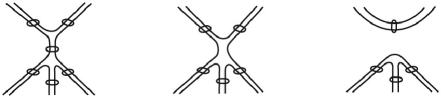
Figure 22.

Similarly, one uses the definition to check the relations (2) and (3). ∎

To state the main result of this section, we also need to define a homomorphism ${\phi}^{\prime}\colon\thinspace BMW_{n}^{\rm skein}\longrightarrow TL_{2n}^{\rm skein}$ (the latter algebra is defined by (2.3)) where the relation between the parameters $q$ in the $BMW$ algebra and $A$ in $TL$ is given by $q=A^{4}$. This map is the “$2$-coloring”: it is defined on tangle generators of $BMW_{n}^{\rm skein}$ by replacing each strand with the Jones-Wenzl projector $P_{2}$. One may check that ${\phi}^{\prime}$ is well-defined directly from definitions (also see [19, p.35]), and this also follows from the commutativity of the diagram below.

Theorem 6.3.

The following diagram commutes.

(6.1)

For convenience of the reader, we recall the notations in the diagram above. The parameter $q$ in the $BMW$ algebras, $Q$ in the chromatic algebra ${\mathcal{C}}_{n}$, $A$ in $TL^{\rm skein}_{2n}$ and $d$ in $TL^{\rm planar}_{2n}$ are related by:

$$q=A^{4},\;\;d=-A^{2}-A^{-2},\;\;Q=q+2+q^{-1}=d^{2}.$$

The traces of various algebras are defined on their respective generators as follows:

$tr_{K}\colon\thinspace BMW_{n}^{\rm skein}\longrightarrow{\mathbb{C}}$ is given by the $SO(3)$ Kauffman polynomial, figure 12.

$tr\colon\thinspace BMW_{n}^{\rm planar}\longrightarrow{\mathbb{C}}$ is the pull-back of $tr_{K}$ via the isomorphism (5.3): $BMW_{n}^{\rm planar}\cong BMW_{n}^{\rm skein}$.

$tr_{\chi}\colon\thinspace{\mathcal{C}}_{n}\longrightarrow{\mathbb{C}}$ is $Q^{-1}$ times the chromatic polynomial of the dual graph, see (3.6).

$tr_{\langle\rangle}\colon\thinspace TL_{2n}^{\rm skein}\longrightarrow{\mathbb{C}}$ is given by the Kauffman bracket defined in (2.3).

$tr_{d}\colon\thinspace TL_{2n}^{\rm planar}\longrightarrow{\mathbb{C}}$, discussed in the section 2, is computed as $d^{\#loops}.$

Proof of theorem 6.3. We begin the proof by showing that the interior diagram of algebra homomorphisms (without the traces) commutes. This amounts to showing that the two maps in the diagram from $BMW^{\rm skein}_{n}$ to $TL^{\rm planar}_{2n}$ send the braiding generator to the same element. The braiding generator $(\backoverslash)$ is mapped by ${\phi}^{\prime}$ to the element of $TL$ shown on the left in figure 23. (The crossings are resolved using (2.3) to get an element of $TL^{\rm planar}_{2n}$.) The other map, $BMW^{\rm skein}\cong BMW^{\rm planar}_{n}\longrightarrow{\mathcal{C}}_{n}\longrightarrow TL^{\rm planar}_{2n}$, sends $(\backoverslash)$ to the linear combination shown on the right in figure 23. (The middle term acquires the coefficient $d$ since the vertex is $4$-valent, see definition 6.1.)

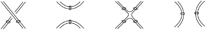
Figure 23.

This identity in the Temperley-Lieb algebra is established in [19, p.35]. We now consider the traces in the diagram (6.1).

Lemma 6.4.

Let $G$ be a planar graph. Then for $Q=d^{2}$,

(6.2) $$tr_{\chi}(G)=Q^{-1}\,{\chi}_{Q}(\widehat{G})\,=\,tr_{d}({\phi}(G)).$$

Therefore, the following diagram commutes:

(6.3)

Proof. The proof (involving the expansion (3.2) of the chromatic polynomial) for trivalent graphs $G$ is given in lemma 2.5 in [10]. Using the contraction-deletion rule (1) in definition 3.2, any graph may be represented as a linear combination of trivalent graphs. The statement then follows from the fact that map $\phi$ and the traces in the diagram above are well-defined. ∎

Observe that the identity in figure 23 shows that the map ${\phi}^{\prime}\colon\thinspace BMW^{\rm skein}_{n}\longrightarrow TL^{\rm skein}_{2n}$ preserves the traces: the evaluation of the $SO(3)$ Kauffman polynomial of the closure of a framed tangle equals the evaluation of the Kauffman bracket of the $2$-coloring of that link. Recall that the isomorphism $BMW_{n}^{\rm planar}\cong BMW_{n}^{\rm skein}$ preserves the trace by definition. Examining the diagram (6.1), one observes that the remaining map $i\colon\thinspace BMW^{\rm planar}_{n}\longrightarrow{\mathcal{C}}_{n}$ preserves the traces as well. This concludes the proof of theorem 6.3. ∎

We state the last observation in the proof above as a corollary. Given a crossing $(\backoverslash)$, one calls $(\hsmoothing)$ its $0$-resolution, and $(\smoothing)$ its $1$-resolution. Given a planar diagram $D$ of a framed link $L$, use (5.3) to express it as a linear combination of planar $4$-valent graphs $G_{i}$. For each $i$, let $p_{i}$ denote the number of $0$-resolutions and $n_{i}$ the number of $1$-resolutions that are used in (5.3) to get the graph $G_{i}$ from the diagram $D$. Let $v(G_{i})$ denote the number of vertices of $G_{i}$.

Corollary 6.5.

[16] Given a framed link $L$, using the notations above the $SO(3)$ Kauffman polynomial $K_{L}$ may be expressed as $K_{L}(q)\;=\;Q^{-1}\sum(-1)^{v(G_{i})}\,q^{p_{i}-n_{i}}\,{\chi}_{\widehat{G_{i}}}(Q)$, where the summation is taken over all $4$-valent planar graphs $G_{i}$ which are the result of applying the formula (5.3) at each crossing of a planar diagram of $L$. Here $Q=(q^{1/2}+q^{-1/2})^{2}$, and ${\chi}_{\widehat{G_{i}}}$ denotes the chromatic polynomial of the graph dual to $G_{i}$.

7. Properties of the chromatic inner product

We use the homomorphism ${\phi}$ to the Temperley-Lieb algebra, defined in 6.1, to study the trace pairing structure on the chromatic algebra ${\mathcal{C}}_{n}$ (introduced in 3.5.)

Lemma 7.1.

The homomorphism ${\phi}\colon\thinspace{\mathcal{C}}_{n}^{\scriptsize{d^{2}}}\longrightarrow TL_{2n}^{d}$ is injective.

Figure 24. ${\phi}$ applied to the graph in figure 10.

Proof. It is easy to see that for any graph $G$ in the rectangle $R$, the terms in the expansion ${\phi}(G)$ are in $1-1$ correspondence with the subsets $S\subset E(G)$ of the set of edges of $G$. More precisely, given such $S$, consider the graph $G_{S}$ whose vertex set consists of all vertices of $G$ and the edge set is $S$. Then the terms of ${\phi}(G)$ correspond (with the coefficient depending on $|S|$) to the boundary of the regular neighborhood of the graphs $G_{S}$. (For an edge $e$, the two terms in the definition of $\phi$ in figure 20 correspond to the two possibilities: $e\in S$, $e\not\in S$.) For more details see the proof of lemma 2.5 in [10].

In lemma 4.4 we showed that (the isotopy classes of) graphs without inner edges in the rectangle $R$ form a basis of ${\mathcal{C}}_{n}$. Suppose a linear combination of such graphs, $\sum{\alpha}_{i}G_{i}$, is in the kernel of ${\phi}$. Consider ${\phi}(G_{i})$ for some $i$, see figure 24 which corresponds to the graph in figure 10. Consider the “leading term” of ${\phi}(G_{i})$, where each edge of $G_{i}$ is replaced by its two parallel copies (the first term in the example in figure 24.) In terms of the correspondence discussed above, this term is given by $S=E(G_{i})$. We claim that this term does not arise in the expansion of any other ${\phi}(G_{j}),$ $j\neq i$.

It is clear that it does not arise as a leading term for any other graph, since each graph is recovered as the spine of its leading term. Since the graphs $G_{j}$ do not have inner edges, it also does not arise as a non-leading term of any ${\phi}(G_{j})$, since any such term involves a “shaded turn-back” – corresponding to a $G_{S}$ which has an isolated vertex on the boundary of $R$, as in the second term in figure 24. Such “shaded turn-backs” cannot be part of a leading term for ${\phi}(G_{i})$ since the graphs with an isolated vertex in the interior of $R$ are trivial in the chromatic algebra (relation $(3)$ in definition 3.2.) This concludes the proof of lemma 7.1. ∎

Corollary 7.2.

Given $Q\geq 0$, the pairing ${\mathcal{C}}^{Q}\otimes{\mathcal{C}}^{Q}\longrightarrow{\mathbb{C}}$, introduced in 3.5, is a positive definite Hermitian product provided that $Q\geq 4$. For $Q$ equal to Beraha numbers $B_{n}=2+2\cos(2{\pi}/(n+1))$, the pairing is positive semidefinite.

The corollary follows from the corresponding statement for the Temperley-Lieb algebra [17] at $d=\sqrt{Q}$ and lemmas 6.4 and 7.1.

We note the intriguing fact that the values of $Q$ for which the Hermitian product on ${\mathcal{C}}^{Q}_{n}$ is positive-definite coincides with the values of $Q$ ($Q\geq 4$) for which the chromatic polynomial of planar graphs is conjectured to be positive [3]. (Of course, $Q=4$ corresponds to the $4$-color theorem.) At Beraha numbers, the trace pairing descends to a positive-definite product on the quotient of ${\mathcal{C}}$ by the trace radical, and it gives rise to the unitary structure of the (doubled) $SO(3)$ TQFT, see section 3.1.

Among the elementary consequences of the corollary above, consider the Cauchy-Schwarz inequality: given two graphs $G,H$ in a disk with an equal number of endpoints on the boundary of the disk, for $Q\geq 4$, $(G,H)^{2}\leq(G,G)\cdot(H,H)$. The inner product is given by gluing two disks along their boundary and computing the chromatic polynomial at $Q\geq 4$ of the dual graph of the resulting graph in the $2$-sphere. This may be loosely formulated as saying that the chromatic polynomial at these values of $Q$ of such graphs is maximized by graphs with a reflection symmetry, a statement that does not seem to follow immediately from the combinatorial definition of the chromatic polynomial.

8. Concluding remarks and questions

We mention a number of questions motivated by our results.

8.1.

The chromatic algebra ${\mathcal{C}}$ defined in this paper provides a natural framework for studying algebraic and combinatorial properties of the chromatic polynomial. We mentioned some of the elementary consequences in sections 3, 4. In [10] we use this algebra to give an algebraic proof of Tutte’s golden identity [33] and to establish chromatic polynomial relations evaluated at Beraha numbers, whose existence was conjectured by Tutte. The chromatic algebra should be useful for a variety of other problems as well, for example it seems likely that it should give new insight into Birkhoff-Lewis equations [3] and the associated Tutte’s invariants [34]. (See also [5] for more details on this subject. The use of the Temperley-Lieb algebra in [5] appears to be different from our approach; it would be interesting to find a connection with our results.)

8.2.

The chromatic algebra and its relations with the TL and BMW algebras should also be useful in analyzing analytic properties of the chromatic polynomial. Specifically, Tutte established the estimate $|{\chi}_{T}({\phi}+1)|\leq{\phi}^{5-k}$, where $T$ is a planar triangulation and $k$ is the number of its vertices. The value ${\phi}+1$ is one of Beraha numbers, $B_{5}$, where $B_{n}=2+2\cos(2{\pi}/n)$. Considering the map ${\phi}\colon\thinspace{\mathcal{C}}_{n}\longrightarrow TL_{2n}$ (defined in section 6), the Beraha numbers correspond to the special values of $d$, $d_{n}=2+2\cos({\pi}/n)$, where the trace radical of the Temperley-Lieb algebra is non-trivial, and is generated by the Jones-Wenzl projector [17]. This algebraic structure may prove useful in determining whether there is an analogue of Tutte’s estimate for other Beraha numbers. (This question is interesting in connection with the observation that the real roots of the chromatic polynomial of large planar triangulations seem to accumulate near the points $\{B_{n}\}$.)

In sections 5, 6 we established a relationship between the $SO(3)$ BMW and chromatic algebras. The former is useful for studying the quantum $SO(3)$ invariants of $3$-manifolds (via their surgery presentation), while the latter is directly related to the chromatic polynomial. It is known [24], [38] that the $SO(3)$ quantum invariants of $3$-manifolds are dense in the complex plane. This motivates the question of whether there may be a related density result for the values of the chromatic polynomial of planar graphs at Beraha numbers.

8.3.

The $SO(N)$ Kauffman polynomial may be viewed as an invariant of planar $4$-valent graphs via the “change of basis” formula (5.3). (Similarly the generators of the $SO(N)$ BMW algebra may be taken to be $4$-valent planar graphs, rather than tangles.) The relations among $4$-valent graphs are then the pullback of the Kauffman relations in figure 12 and of the last two Reidemeister moves under (5.3).

In this paper we show that in the case $N=3$ all of these relations follow from the chromatic relations in definition 3.2. We also discuss the special case $N=4$ in [10, section 4], relating $BMW(4)$ with $TL\times TL$. It is an interesting question whether there is a nice combinatorial/geometric interpretation of the $SO(N)$ invariant of graphs for other values of $N$ involving unlabeled graphs. (A different approach is taken in [22] in the rank $2$ case where the graph edges have different labels.)

8.4.

In this paper we define and investigate some of the properties of the map from the $SO(3)$ BMW algebra to the chromatic algebra, $i\colon\thinspace BMW_{n}\longrightarrow{\mathcal{C}}_{n}$, see theorem 5.1. It would be interesting to establish a precise relationship between these algebras. As indicated in remark 5.4, we believe this homomorphism is injective but not surjective. (From the TQFT perspective, an interesting question is whether these two algebras are Morita equivalent.) It follows from lemma 6.4 that at special values of $Q=2+2\cos(2{\pi}j/n)$, the pull-back of the Jones-Wenzl projector from the Temperley-Lieb algebra via the homomorphism $\phi$ is in the trace radical of the chromatic algebra. A question important from the perspective of finding linear relations among the values of the chromatic polynomial of planar graphs (see [10]) is whether this pull-back of the Jones-Wenzl projector generates the entire trace radical of the chromatic algebra.

References

- [1] R.J. Baxter, Exactly Solved Models in Statistical Mechanics (Academic, London, 1982)
- [2] B. Bollobas, Modern graph theory, Springer, 1998.
- [3] G.D. Birkhoff and D.C. Lewis, Chromatic polynomials, Trans. Amer. Math. Soc. 60 (1946), 355-451.
- [4] J. Birman and H. Wenzl, Braids, link polynomials and a new algebra, Trans. Amer. Math. Soc. 313 (1989), 249–273.
- [5] S. Cautis and D. Jackson, The matrix of chromatic joins and the Temperley-Lieb algebra, J. Combin. Theory Ser. B 89 (2003), 109–155.
- [6] L. Chim and A. B. Zamolodchikov, Integrable field theory of q state Potts model with , Int. J. Mod. Phys A 7 (1992) 5317.
- [7] P. Fendley, Topological order from quantum loops and nets, Ann. Physics 323 (2008), 3113-3136. [arXiv:0804.0625]
- [8] P. Fendley and E. Fradkin, Realizing non-Abelian statistics in time-reversal-invariant systems, Phys. Rev. B 72 (2005) 024412 [arXiv:cond-mat/0502071]
- [9] P. Fendley and J.L. Jacobsen, Critical points in coupled Potts models and critical phases in coupled loop models, J. Phys. A: Math. Theor. 41 (2008) 215001 [arXiv:0803.2618]
- [10] P. Fendley and V. Krushkal, Tutte chromatic identities from the Temperley-Lieb algebra, Geom. Topol. 13 (2009), 709-741 [arXiv:0711.0016]
- [11] P. Fendley and N. Read, Exact S-matrices for supersymmetric sigma models and the Potts model, J. Phys. A 35 (2003) 10675 [arXiv:hep-th/0207176]
- [12] L. Fidkowski, M. Freedman, C. Nayak, K. Walker, Z. Wang, From String Nets to Nonabelions, cond-mat/0610583.
- [13] C.M. Fortuin and P.W. Kasteleyn, On The Random Cluster Model. 1. Introduction And Relation To Other Models, Physica 57, 536 (1972).
- [14] M. Freedman, A magnetic model with a possible Chern-Simons phase, Comm. Math. Phys. 234 (2003), 129–183 [arXiv:quant-ph/0110060]
- [15] M. Freedman, C. Nayak, K. Walker, Z. Wang, On Picture (2+1)-TQFTs, arXiv:0806.1926.
- [16] F. Jaeger, On some graph invariants related to the Kauffman polynomial, Progress in knot theory and related topics. Paris: Hermann. Trav. Cours. 56, 69-82 (1997).
- [17] V.F.R. Jones, Index for subfactors, Invent. Math. 72 (1983), 1-25.
- [18] V.F.R. Jones, Planar algebras, arXiv:math/9909027.
- [19] L.H. Kauffman and S.L. Lins, Temperley-Lieb recoupling theory and invariants of -manifolds, Princeton University Press, Princeton, NJ, 1994.
- [20] L.H. Kauffman and P. Vogel, Link polynomials and a graphical calculus, J. Knot Theory Ramifications 1 (1992), 59–104.
- [21] W.M. Koo and H. Saleur, Fused Potts models, Internat. J. Modern Phys. A 8 (1993), 5165–5233.
- [22] G. Kuperberg, Spiders for rank Lie algebras, Comm. Math. Phys. 180 (1996), 109–151.
- [23] M. Larsen and Z. Wang, Density of the SO(3) TQFT representation of mapping class groups, Comm. Math. Phys. 260 (2005), 641–658.
- [24] M. A. Levin and X. G. Wen, String-net condensation: A physical mechanism for topological phases Phys. Rev. B 71 (2005) 045110 [arXiv: cond-mat/0404617]
- [25] P. P. Martin and D. Woodcock, The partition algebras and a new deformation of the Schur algebras, J. Algebra 203 (1998), 91-124.
- [26] J. Murakami, The Kauffman polynomial of links and representation theory. Osaka J. Math. 24 (1987), 745–758.
- [27] N. Reshetikhin, V. Turaev, Invariants of -manifolds via link polynomials and quantum groups, Invent. Math. 103 (1991), 547-597.
- [28] F.A. Smirnov, Exact S matrices for phi(1,2) perturbated minimal models of conformal field theory Int. J. Mod. Phys. A 6 (1991) 1407.
- [29] H. N. V. Temperley and E. H. Lieb, Relations between the ’percolation’ and ’colouring’ problem and other graph-theoretical problems associated with regular planar lattices: some exact results for the ’percolation’ problem, Proc. Roy. Soc. Lond. A 322, 251 (1971).
- [30] V. Turaev, Quantum invariants of knots and 3-manifolds, Walter de Gruyter & Co., Berlin, 1994.
- [31] V. Turaev and O. Viro, State sum invariants of manifolds and quantum symbols, Topology 31 (1992), 865-902.
- [32] W.T. Tutte, On chromatic polynomials and the golden ratio, J. Combinatorial Theory 9 (1970), 289–296.
- [33] W.T. Tutte, More about chromatic polynomials and the golden ratio, Combinatorial Structures and their Applications, 439-453 (Proc. Calgary Internat. Conf., Calgary, Alta., 1969)
- [34] W.T. Tutte, On the Birkhoff-Lewis equations, Discrete Math., 92 (1991), 417-425.
- [35] K. Walker, talk given at IPAM conference “Topological Quantum Computing”, available at https://www.ipam.ucla.edu/schedule.aspx?pc=tqc2007
- [36] K. Walker, On Witten’s -manifold invariants, available at http://canyon23.net/math/
- [37] E. Witten, Quantum field theory and the Jones polynomial, Commun. Math. Phys. 121 (1989) 351.
- [38] H. Wong, quantum invariants are dense, preprint.
- [39] S. Yamada, An operator on regular isotopy invariants of link diagrams, Topology 28 (1989), 369–377.