Strong correlation effects in diatomic molecular electronic devices

Abstract

We present a qualitative model for a fundamental process in molecular electronics: the change in conductance upon bond breaking. In our model a diatomic molecule is attached to spin-polarized contacts. Employing a Hubbard Hamiltonian, electron interaction is neglected in the contacts and explicitly considered in the molecule, enabling us to study the impact of electron interaction on the molecular conductance. In the limit where the electron repulsion is strong compared to the binding energy (as it becomes the case upon dissociation) electron transmission in strongly suppressed compared to the non-interacting case. However, the spin-polarized nature of the contacts introduces a coupling between the molecular singlet and triplet states. This coupling in turn yields additional resonances in the transmission probability that significantly reduce the energetic separation appear between resonances. The ramifications of our results on transport experiments performed on nanowires with inclusions $H_{2}$ are discussed.

Molecular electronics JGA00 ; N01 ; NR03 ; HR03 ; CHH07 offers new perspectives for the construction of electronic devices. Even though some quantum effects, such as tunneling, are sometimes undesirable in conventional electronics, molecular electronic devices (MEDs) systematically exploit quantum effects and are therefore suitable for the construction of devices on the atomic scale. Another field that may contribute to the development of new electronic devices is spintronics (for reviews see, e.g., Zuticetal04RMP ; Bratkovsky08RPP ), where spin and charge transport are investigated on a mesoscopic scale. Molecular spintronics emerged in experimental and theoretical studies as a result of recent combination of molecular electronics and spintronics Rochaetal05 ; Seneoretal07JPCM . Most theoretical approaches to MED’s are based on effective one-electron theories MKR94 ; D95 ; NDL95 ; XDR01 ; TGW01a ; BMO02 ; KBY04 ; EZ05 ; SGP06 and do not properly account for electron correlation effects EZ05 ; kbe06 . Providing a remedy for this shortcoming remains a formidable challenge. Recent work to address this issue invokes, for instance, the configuration interaction method to calculate the conductance. While the proper inclusion of the infinite contacts remains an unsolved problem in this approach, correlation effects are accounted for. Non-equilibrium Green’s function techniques have also been employed T08 in conjunction with model Hamiltonians to understand correlation effects. Here, we follow a similar route. We use the recently developed source-sink potential method (SSP) GEZ07 ; Ernzerhof07 to a model Hamiltonian involving Hubbard term to address the problem of electron correlation in molecular conductors.

One of the most fundamental phenomena undergone by molecules is that of bond formation and bond breaking. Chemical bonds are sometimes stretched and broken by mechanical force in break junction experiments ME85 ; RAP96 . In this letter, we address the breaking of a chemical bond in a diatomic molecule, which constitutes part of a MED. We provide an answer to the question of how the conductance of a diatomic molecule changes during bond breaking. In a simple molecular orbital picture (appropriate for non-interacting electrons), during the breakage of a bond, the binding and antibinding orbital approach each other in energy until they become degenerate in the separated atom limit. Therefore, electron interaction effects become increasingly important on the scale of the single-electron energies and a strongly correlated system is obtained. This system cannot be properly described by the Kohn-Sham reference determinant PY89 ; DG90 , or any other single-particle description, appropriate for a non-degenerate ground state. As a consequence, the popular combination of DFT and non-equilibrium Green’s function technique KMR94b ; D95 ; Tayloretal01PRB to model transport in MEDs is inadequate.

The system under consideration is comprised of two semi-infinite non-interacting contacts. The boundary conditions of the problem are chosen such that in the left contact (L) we have an incoming Bloch wave that provides an electron current towards the contact-molecule interface. At the interface, the incoming wave is partially reflected from and partially transmitted through the molecule. In the present work, we admit only infinitesimal voltage differentials, i.e., we consider the zero-bias conductance and assume that the ambient temperature is zero. We will be concerned with noninteracting spin-polarized contacts which contain up-spin electrons only. This requirement can be fulfilled experimentally by using ferromagnetic leads with parallel configurations Seneoretal07JPCM . Also, external magnets or impurities in the contacts can be employed to spin-polarize the contacts Sachrajdaetal03PRL ; Rochaetal05 . The molecule constitutes a subsystem in which the electrons repel each other and correlation effects are accounted for by means of a multi-configurational description. By constraining the wave function, we ensure that only a single electron can escape from the molecule into the contacts. Having two electrons in the contact would mean that the wave function in the contact is a multi-electron and not a single-electron one. Apart from spin-polarized contacts, our model might be relevant to experiments CHM06 ; CHM04 , where hydrogen molecules are confined between metal wires. The charging energy of the molecule in such wires might result in Coulomb blockade and explain the appearance of just one open channel. While the contacts are non-interacting one-electron regions, the interface between the molecule and the contact requires some attention. The interface becomes relevant for configurations in which one electron is on the molecule and the other one is in the contact. Since there are only up-spin electrons in the contacts, the electron remaining in the molecule has down spin. One might think that the electrons are either singlet or triplet coupled, but in fact a mixture of singlet and triple state is required to account for the present electron distribution. This is because the contact electron is an up-spin electron which cannot be realized with a triplet or a singlet coupled configuration, but with an appropriate superposition of the two. This is an important point for the basis set selection since in our approach, we calculate the stationary states of a model Hamiltonian in finite basis set representation.

The configuratons that we consider as basis functions are determined such that they can describe known simple limits. For our purposes, the most important such limit is the dissociated molecule where the two atoms of the molecule are decoupled. The incoming up-spin electron in the left contact is completely reflected and it does not reach the right contact. Furthermore, due to electron-electron repulsion, the up-spin and down-spin electrons are localized in the left and right part of the system respectively. Another obvious limit is the non-interacting on. In this case, we have to recover the known transmission probability ($T(E)$) curve (see, e.g. GEZ07 ) exhibiting a resonance due to the HOMO and one due to the LUMO orbital. One of the key results obtained from our model is that the separation between the HOMO and the LUMO resonance is drastically reduced as the electron interaction is introduced.

We study $T(E)$ of this system as a function of the energy with which the electron travels through the contact, i.e., as a function of the Fermi energy at zero temperature. Alternatively, one might think of a gated device in which the Fermi energy of the contacts is kept fixed and the molecular part of the MED is shifted in energy by a gate voltage. In doing so, we obtain resonances that are related to the molecular states. Therefore, before investigating the MED, we consider the isolated molecule (i.e. sans contacts) subject to electron-electron interaction. The Hamiltonian of the isolated molecule is given by

$$\sum_{\sigma}\left(\beta_{M}c^{\dagger}_{a\sigma}c_{b\sigma}+H.c.\right)+\sum_{\alpha\sigma}h_{\alpha}n_{\alpha\sigma}+\frac{1}{2}\sum_{\alpha\sigma\sigma^{\prime}}Un_{\alpha\sigma}n_{\alpha\sigma^{\prime}}$$ (1)

where the operator $c^{\dagger}_{\alpha\sigma}$ ($c_{\alpha\sigma}$) with $\alpha$=a,b creates(destructs) an electron in the molecular sites a and b. $\sigma$ stands for the spin degrees of freedom and $n_{\alpha\sigma}$ is the number operator. $U$ is the Hubbard electron-electron repulsion parameter and $\beta_{M}$ the intramolecular hopping parameter. The diagonal elements $h_{a}$ and $h_{b}$ are set equal to zero, thus we will be concerned with a homonuclear molecule. We consider a finite Hilbert space in which to diagonalize the molecular Hamiltonian. The singlet configurations that form the basis functions can be divided into two ionic ones with both electrons localized on either atom $a$ or atom $b$ and a covalent one with one electron per atom, i.e.,

$$\Phi_{1} = \frac{1}{\sqrt{2}}\mid aa>(\mid\uparrow\downarrow>-\mid\downarrow\uparrow>),$$

$$\Phi_{2} = \frac{1}{2}(\mid ab>+\mid ba>)(\mid\uparrow\downarrow>-\mid\downarrow\uparrow>),$$

$$\Phi_{3} = \frac{1}{\sqrt{2}}\mid bb>(\mid\uparrow\downarrow>-\mid\downarrow\uparrow>).$$ (2)

This basis enables us to describe the ground state (doubly occupied HOMO) and two excited states where one electron or two electron are promoted to the LUMO, respectively. The Hamiltonian in the finite subspace is then given by AB02

$${\bf H}=\left(\begin{array}[]{ccc}U&\sqrt{2}\beta_{M}&0\\ \sqrt{2}\beta_{M}&0&\sqrt{2}\beta_{M}\\ 0&\sqrt{2}\beta_{M}&U\end{array}\right).$$

Solving the eigenvalue equation for the isolated molecule, we obtain three eigenvalues,

$$E_{0} = \frac{1}{2}\left(U-\sqrt{U^{2}+16\beta_{M}^{2}}\right)$$

$$E_{1} = U$$

$$E_{2} = \frac{1}{2}\left(U+\sqrt{U^{2}+16\beta_{M}^{2}}\right).$$ (3)

As $U$ is increased, the ground state raises in energy to reach zero for $U=\infty$. In the corresponding wave function, there is one electron on each atom, completely eliminating the repulsion energy. Due to this localization of the electrons there is no binding interaction between the atoms either. Furthermore, since our reservoirs are spin polarized, the triplet state of the system

$$\Phi_{4}=\frac{1}{2}(\mid ab>-\mid ba>)(\mid\uparrow\downarrow>+\mid\downarrow\uparrow>).\\$$ (4)

also plays an important role. The energy of this state is zero, independent of the value of $U$. In the limit where $\beta_{m}$ goes to zero or where $U$ goes to infinity, the singlet ground state and the triplet state become degenerate. For the MED this implies that in these limits, a superposition of singlet and triplet state determines the transmission probability through the system.

We can now turn our attention to the MED, which consists of the desribed diatomic molecule attached to the left (L) and right (R) spin-polarized semi-infinite contacts in serial arrangement. The contacts are modeled by one-dimensional chains of atoms, nearest neighbor coupled with strength $\beta_{C}$. The diagonal elements of the contact atoms are set to zero. L and R in turn, are coupled to atom $a$ and $b$, respectively, through the parameter $\beta_{CM}$. Employing the SSP approach GEZ07 to eliminate the infinite contacts, we obtain the Hamiltonian

$$H=h_{\uparrow}+h_{\downarrow}+V_{\uparrow\downarrow}$$ (5)

where

$$h_{\uparrow} = \Sigma_{L}n_{L\uparrow}+\Sigma_{R}n_{R\uparrow}+\beta_{CM}c^{\dagger}_{L\uparrow}c_{a\uparrow}+H.c.+$$ (6)

$$\beta_{CM}c^{\dagger}_{R\uparrow}c_{b\uparrow}+H.c.+\beta_{M}c^{\dagger}_{a\uparrow}c_{b\uparrow}+H.c.$$

$$h_{\downarrow} = \beta_{CM}c^{\dagger}_{L\downarrow}c_{a\downarrow}+H.c.+\beta_{CM}c^{\dagger}_{R\downarrow}c_{b\downarrow}+H.c.+$$ (7)

$$\beta_{M}c^{\dagger}_{a\downarrow}c_{b\downarrow}+H.c.$$

and

$$V_{\uparrow\downarrow}=\sum_{\alpha}Un_{\alpha\uparrow}n_{\alpha\downarrow}.$$ (8)

The operators $c^{\dagger}_{\alpha\sigma}$ ($c_{\alpha\sigma}$) with $\alpha$=$a$, $b$ and $c^{\dagger}_{\beta\sigma}$ ($c_{\beta\sigma}$) with $\beta$=L,R create(destruct) an electron in the molecular sites a and b and contacts L and R respectively. The source $\Sigma_{L}=\beta_{C}\frac{e^{-iq}+re^{iq}}{1+r}$ and sink $\Sigma_{R}=\beta_{C}e^{iq}$ potential GEZ07 appearing in the Hamiltonian are applied to the first atom of L and R respectively. In these potentials, $q=arccos\left(\frac{E}{2\beta_{C}}\right)$. They represent the infinite parts of single-electron contacts in a rigorous manner GEZ07 .

Building on the discussions above, our finite dimensional Hilbert space consists of the for configurations listed in Eqs. 2 and 4. We additionally include configurations that are obtained from the described ones by exciting the up-spin electron from atom $a$ or atom $b$ into the contacts. The resulting eight configurations are depicted in Fig. 1.

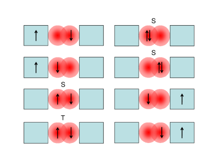
Figure 1: This figure schematically shows the states used to construct the Hamiltonian matrix for the full MED. The arrows represent the spin orientation of the electron and their positions depict where the electron is localized within the MED. The letters denote whether the diagram corresponds to a singlet or triplet.

The Hamiltonian Eq. 5 is now represented in the space of the configurations,

$$\left(\begin{array}[]{cccccccc}\Sigma_{L}&\beta_{M}&0&0&\beta_{CM}&0&0&0\\ \beta_{M}&\Sigma_{L}&\frac{\beta_{CM}}{\sqrt{2}}&\frac{\beta_{CM}}{\sqrt{2}}&0&0&0&0\\ 0&\frac{\beta_{CM}}{\sqrt{2}}&0&0&\sqrt{2}\beta_{M}&\sqrt{2}\beta_{M}&\frac{\beta_{CM}}{\sqrt{2}}&0\\ 0&\frac{\beta_{CM}}{\sqrt{2}}&0&0&0&0&-\frac{\beta_{CM}}{\sqrt{2}}&0\\ \beta_{CM}&0&\sqrt{2}\beta_{M}&0&U&0&0&0\\ 0&0&\sqrt{2}\beta_{M}&0&0&U&0&\beta_{CM}\\ 0&0&\frac{\beta_{CM}}{\sqrt{2}}&-\frac{\beta_{CM}}{\sqrt{2}}&0&0&\Sigma_{R}&\beta_{M}\\ 0&0&0&0&0&\beta_{CM}&\beta_{M}&\Sigma_{R}\\ \end{array}\right),$$

Having defined our model Hamiltonian, we can proceed to describe how the reflection coefficients are calculated. The transmission probability $T(\epsilon)$ gives the probability of an electron arriving with an energy $\epsilon$ to pass through the molecule into the right contact. $T(\epsilon)$ is related to the reflection coefficient $r(\epsilon)$ by $T(\epsilon)=1-|r(\epsilon)|^{2}$. $r(\epsilon)$ is an as of yet unknown parameter in the potential $\Sigma_{L}$. To obtain $r(\epsilon)$, we start from the eigenvalue equation

$$H(\epsilon,r)\Psi=E\Psi,$$ (9)

where $E$ is the total energy of the system. $\epsilon$ takes a real value of our choice. The total energy of the system can now be written as $E=E^{N-1}+\epsilon$ KD80 ; EBP96 , where $E^{N-1}$ is the energy of the $N-1$-electron system obtained by removing the up-spin electron. In the present example $E=E^{N-1}$ can take on two different values, one being the orbital energy of the binding and the other being the orbital energy of the anti binding orbital. Since we are interested in the state that emerges from the molecular ground state, we set $E=E_{b}^{N-1}+\epsilon$, where $E_{b}^{N-1}$ is the energy of the binding orbital in the isolated molecule. Therefore, Eq. 9 becomes

$$H(\epsilon,r)\Psi=(E_{b}^{N-1}+\epsilon)\Psi.$$ (10)

The corresponding secular equation is

$$Det(H(\epsilon,r)-(E_{b}^{N-1}+\epsilon))=0.$$ (11)

Since the value of $\epsilon$ represents a boundary condition that we specify, Eq. 11 determines the unknown $r$ in terms of the variable $\epsilon$.

First, we verify that our model reproduces the known answer of $T(\epsilon)=1$ the non-interacting, perfect ballistic conductor. Therefore, we chose a homogeneous linear wire with $\beta_{C}=\beta_{CM}=\beta_{M}=-2$ and $U=0$. Note that we use arbitrary energy units as only the relative proportions of the parameters are of significance. Calculation of $T(\epsilon)$ according to the above procedure yields the desired solution (red dashed curve in Fig. 2).

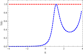
Figure 2: This figure shows $T(\epsilon)$ for a homogeneous non-interacting wire as a function of Fermi energy $\epsilon$. Two solutions are found and represented in different colors. The second solution (blue curve) corresponds to a wave function that exhibits a localized excited state in the ”molecule”.

We also find a second solution (blue dashed curve) that varies strongly. This curve originates from the many-electron basis employed for the central region (supermolecule) of the MED comprising of the molecule plus the two contact atoms explicitly considered. Even when $U$=0, we still have a many-electron wave function in the supermolecular region. This means that we have to expect resonances that correspond to local excitations in the supermolecule. Such excited states also couple to the contacts and yield a $T(\epsilon)$ that is neither constant nor equal to one. In the localized excited state, the down-spin electron is in the anti-bond and the incoming electron passes through the HOMO. Since such a local excitation is unlikely to remain localized in a system rather than diffusing into the contacts, we think that the second curve is not observable. In our simple treatment, we lack the basis functions in the contacts that would permit the local excitation to decay. While this excitation by itself might not necessarily be significant, its impact on the non-excited solution is. We pursue this issue for inhomogeneous MEDs, where it is realistic to have a strong electron-electron interaction in only the molecular part of the MED.

We now consider an inhomogeneous system, where the contact atoms are more tightly bound $\beta_{C}=-10$ than the remaining ones ($\beta_{CM}=-2,\beta_{M}=-2$). One might think of this system as a stretched break junction, with a weakened molecule-contact and molecular bond. The corresponding $T(\epsilon)$ curves for vanishing $U$ are shown in Fig. 3. The blue dashed curve on the left, emerging from the ground state of the molecule has a resonance at the HOMO energy and a second one at the LUMO energy. The separation of these orbitals in the isolated molecule is 4($2\beta_{M}$) and this separation is essentially preserved Ernzerhof07 in the MED since the value of $\beta_{CM}$ is large, this is because, we are close to the wide band limit where the contacts become featureless. Note that this curve coincides with the one obtained from a non-interacting theory (e.g., SSP as described in Ref. Ernzerhof07 ). The red dashed curve, emerging from an excited state of the molecule shows a resonance at the LUMO energy and a further resonance corresponding to a doubly occupied LUMO orbital. The red-dashed curve is absent in an independent electron treatment. Even though the interaction parameter is $U=0$, we still observe excited states (and the corresponding resonances) for the reasons discussed above. As in the example of a homogeneous wire, the excited-localized state would probably be quenched by the contacts and difficult to observe experimentally, unless the coupling between the contacts and the molecule is small. For finite $U$, the excited states couples with the ground state and therefore, becomes noticeable in the $T(\epsilon)$ curve corresponding to the ground state.

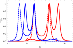
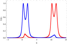
Figure 3: Left panel shows $T(\epsilon)$ for an inhomogeneous wire containing a diatomic molecule for $U$=0 (dashed curves) and for $U$=4 (solid curves) as a function of Fermi energy $\epsilon$. Right panel depicts the same system for $U$=8

In the interacting system that we are going to consider next we set $U=4$. This choice is motivated by the fact that in the isolated hydrogen molecule, $U$ has to be twice as large as $|\beta_{M}|$ in order to describe the certain properties of the hydrogen molecule CL07 . For an interacting system, with $U=4$, the ground state is destabilized compared to the non-interacting system (see Eq. 3). Furthermore, the separation between the ground- and the first-excited state increases to  6.5. Therefore, naively one would expect a corresponding increase in the separation between the resonances in the $T(\epsilon)$ curve. We investigate this question with the help of the solid curves in Fig. 3 where $U=4$. Surprisingly, the separation between the first two resonances diminishes even compared to the $U=0$ case. This is due to the mixing of states that yield the coinciding resonances in the $T(\epsilon)$ curve of the non-interacting case. Furthermore, the second solution (red solid curve) is shifted towards higher energies due to the electron-electron repulsion. The states in the red solid curve have large ionic contributions in which two electrons are localized on one molecular atom. Increasing $U$ even further to a value of $U=8$ yields the curve depicted in the right panel of Fig. 3. The gap between the two resonance diminishes further and the resonances in the red curve move higher in energy. Eventually, when the two resonances in the blue curve start to overlap with each other destructive interference sets in, leading to the disappearance of $T(\epsilon)$. In Fig. 4 we show the transmission results for $U=32$. In the large $U$ limit, the ionic states described above acquire an infinite energy due to electron repulsion. The two covalent states, having an electron on atom $a$ and a second one on atom $b$ in a singlet and triplet spin-coupling, become degenerate. As a consequence of this degeneracy, we get a destructive interference between the molecular singlet and triplet state leading to a localization of up-spin electron and down-spin electron on atom $a$ or atom $b$ respectively. This interpretation can be verified by examining the coefficients if the various configurations in the wave function.

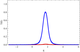
Figure 4: $T(\epsilon)$ for an inhomogeneous wire approaching the strong correlation limit ($U=32$) as a function of Fermi energy $\epsilon$.

Next, we consider the case where the coupling between the molecule and the contacts is weak $\beta_{CM}<1$. We obtain a $T(\epsilon)$ curve that resembles the one of Fig. 3, except, of course, the peak widths are reduced. Increasing the interaction parameter($U=4$) yields similar results to the ones shown in Fig. 3. Again, we observe a dramatic reduction of the separation between the first two resonances as compared to the non-interacting case.

Now we turn to the dissociation limit, where the coupling between the molecular atoms ($\beta_{M}$) approaches zero. In this case, on the scale of the $\beta_{M}$, the importance of the repulsion parameter $U$ increases and we enter the strong-correlation regime. Therefore, we expect the same qualitative behavior as in the strongly interacting case.

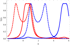
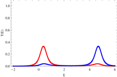
Figure 5: The left plot shows $T(\epsilon)$ for weakly coupled ($\beta_{M}=-1$) molecular atoms. The dashed curves correspond to non-interacting system. The solid curves are obtained for the same system with $U=4$. The right plots illustrates $T(\epsilon)$ for very weakly coupled molecular atoms ($\beta_{M}=-1/2$) with $U=4$.

In the case where $U=0$ and $\beta_{M}=-1$ (Fig. 5) all the resonances are compressed into a smaller energy interval as expected. This implies that electron interaction is going to have a large effect, since all these close resonances are going to be coupled. The solid blue curve, where $U=4$ yields two coinciding resonances, or equivalently, the gap between the first two resonances disappeared completely. For cases where the Fermi level is located between the HOMO and LUMO level of the non-interacting case, a strong conductance enhancement would be obtained. As already explained, this enhancement is due to the indirect impact of the molecular triplet state. Reducing the absolute value of $\beta_{M}$ even further ($\beta_{M}=-1/2$) in the right plot of Fig. 5) leads to a strong suppression of the $T$ in the interacting case as opposed to the non-interacting case. We are again approaching the strongly-correlated limit and naturally, the $T(\epsilon)$ curve resembles the one of Fig. 4. The preceding discussion underlines the statement made in the introduction, that bond breaking turns the system into a strongly correlated one. Therefore, even if in reality, the value of the parameter $U$ is fixed, stretching the bond amounts to an effective increase of the parameter relative to the atom-atom coupling. In general, one would expect that electron-electron interaction effects reduce $T(\epsilon)$ kbe06 . This is indeed what we observe, except in cases where the electron repulsion mixes in further states as it is the case here with the molecular triplet states.

In conclusion, our understanding of correlation effects on the transmission probability of molecular conductors is still quite limited. In this letter, we provided a qualitative model of correlation effects. We focused on the molecular part of the MED and considered the simplest possible way of introducing electron interaction effects therein. In the interacting case, we uncovered a new, unexpected resonance that originates from the lowest triplet state of the isolated molecule. In the presence of electron repulsion, this state is coupled to the molecular ground state to drastically reduce the gap between the HOMO and the LUMO resonance that would be observed in a non-interacting system.

In our model, the contacts were assumed to be spin polarized. Nonetheless, we argue that our model calculations pertain to realistic systems. Indeed, recent experiments CHM04 ; CHM06 in which $H_{2}$ molecules are inserted between gold wires give rise to the speculation that there is only one spin channel open. Spin-polarization in the contacts appears to be attainable with experimental techniques as well. The fact that the conductance is suppressed gradually in our calculations in the strongly correlated limit as a function of $\beta_{M}$ instead of collapsing abruptly serves as further evidence that our results are in line with the experimental data Smitetal02 ; CHM06 ; Schonenebergeretal06NL ; Xiaetal08NL . Therefore, we have reason to believe that our model sheds light on electron interaction effects despite its seemingly unsophisticated nature.

We gratefully acknowledge financial support provided by NSERC.

References

- (1) Joachim, G.; Ginzewski, J. K.; Aviram, A. Nature 2000, 408, 541–548.
- (2) Nitzan, A. Annu. Rev. Phys. Chem. 2001, 52, 681–750.
- (3) Nitzan, A.; Ratner, M. A. Science 2003, 300, 1384–1389.
- (4) Heath, J. R.; Ratner, M. A. Phys. Today 2003, 56, 43–49.
- (5) Chen, F.; Hihath, J.; Huang, Z.; Li, X.; Tao, N. J. Annu. Rev. Phys. Chem. 2007, 58, 535.
- (6) Zutic, I.; Fabian, J.; Sarma, S. D. Rev. Mod. Phys. 2004, 76, 323–410.
- (7) Bratkovsky, A. M. Rep. Prog. Phys. 2008, 71, 026502.
- (8) Rocha, A. R.; Garcia-Suarez, V. M.; Bailey, S. W.; Lambert, C. J.; Ferrer, J.; Sanvito, S. Nature Materials 2005, 4, 335–339.
- (9) Seneor, P.; Bernard-Mantel, A.; Petroff, F. J. Phys.: Condens. Matter 2007, 19, 165222.
- (10) Mujica, V.; Kemp, M.; Ratner, M. A. J. Chem. Phys. 1994, 101, 6856–6864.
- (11) Datta, S. Electronic Transport in Mesoscopic Systems; Cambridge University Press, 1995.
- (12) Lang, N. D. Phys. Rev. B 1995, 52, 5335–5342.
- (13) Xue, Y. Q.; Datta, S.; Ratner, M. A. J. Chem. Phys. 2001, 115, 4292–4299.
- (14) Taylor, J.; Guo, H.; Wang, J. Phys. Rev. B 2001, 63, 121104(R).
- (15) Brandbyge, M.; Mozos, J.-L.; Ordejón, P.; Taylor, J.; Stokbro, K. Phys. Rev. B 2002, 65, 165401.
- (16) Ke, S.-H.; Baranger, H. U.; Yang, W. Phys. Rev. B 2004, 70, 085410.
- (17) Ernzerhof, M.; Zhuang, M. Int. J. Quantum Chem. 2005, 101, 557–563.
- (18) Solomon, G. C.; Gagliardi, A.; Pecchia, A.; Frauenheim, T.; Di-Carlo, A.; Reimers, J. R.; Hush, N. S. J. Chem. Phys. 2006, 125, 184702.
- (19) Koentopp, M.; Burke, K.; Evers, F. Phys. Rev. B 2006, 73, 121403.
- (20) Thygesen, K. S. Phys. Rev. Lett. 2008, 100, 166804.
- (21) Goyer, F.; Ernzerhof, M.; Zhuang, M. J. Chem. Phys. 2007, 126, 144104.
- (22) Ernzerhof, M. J. Chem. Phys. 2007, 127, 204709.
- (23) Moreland, J.; Ekin, J. W. J. Appl. Phys. 1985, 58, 3888–3895.
- (24) van Ruitenbeek, J. M.; Alavarez, A.; neyro, I. P.; Grahmann, C.; Joyez, P.; Devoret, M. H.; Esteve, D.; Urbina, C. Rev. Sci. Instrum. 1996, 67, 108–111.
- (25) Parr, R. G.; Yang, W. Density-Functional Theory of Atoms and Molecules; Oxford University Press: Oxford, 1989.
- (26) Dreizler, R. M.; Gross, E. K. U. Density Functional Theory; Springer Verlag: Berlin, 1990.
- (27) Kemp, M.; Mujica, V.; Ratner, M. A. J. Chem. Phys. 1994, 101, 5172–5178.
- (28) Taylor, J.; Guo, H.; Wang, J. Phys. Rev. B 2002, 63, 245407.
- (29) Pioro-Ladriere, M.; Ciorga, M.; Lapointe, J.; Zawadzki, P.; Korkusinski, M.; Hawrylak, P.; Sachrajda, A. S. Phys. Rev. Lett. 2003, 91, 026803.
- (30) Csonka, S.; Halbritter, A.; Mihaly, G. Phys. Rev. B 2006, 73, 075405.
- (31) Csonka, S.; Halbritter, A.; Mihály, G.; Shklyarevskii, O. I.; Speller, S.; van Kempen, H. Phys. Rev. Lett. 2004, 93, 016802.
- (32) Alvarez-Fernández, B.; Blanco, J. A. Eur. J. Phys. 2002, 23, 11–16.
- (33) Katriel, J.; Davidson, E. R. Proc. Natl. Acad. Sci. USA 1980, 77, 4403.
- (34) Ernzerhof, M.; Burke, K.; Perdew, J. P. J. Chem. Phys. 1996, 105, 2798.
- (35) Chiappe, G.; Louis, E.; SanFabi n, E.; Verges, J. A. Phys. Rev. B 2007, 75, 195104–1–195104–6.
- (36) Smit, R. H. M.; Noat, Y.; Untiedt, C.; Lang, N. D.; van Hemert, M. C.; van Ruitenbeek, J. M. Nature 2002, 419, 906–909.
- (37) Gonzalez, M. T.; Wu, S.; Huber, R.; van der Molen, S. J.; Schonenberger, C.; Calame, M. Nano Lett. 2006, 6, 2238–2242.
- (38) Xia, J. L.; Diez-Perez, I.; Tao, N. J. Nano Lett. 2008, 8, XXX.