Cryptography in a Quantum World

Abstract

Quantum computing had a profound impact on cryptography. Shor’s discovery of an efficient quantum algorithm for factoring large integers implies that nearly all existing classical systems based on computational assumptions can be broken, once a quantum computer is built. It is therefore imperative to find other means of implementing secure protocols. This thesis aims to contribute to the understanding of both the physical limitations, as well as the possibilities of cryptography in the quantum setting. To this end, we first investigate two notions that are crucial to the security of quantum protocols: uncertainty relations and entanglement. How can we find good uncertainty relations for a large number of measurement settings? How does the presence of entanglement affect classical protocols? And, what limitations does it impose on implementing quantum protocols? Finally, can we circumvent some of those limitations using realistic assumptions?

Cryptography in a Quantum World

ILLC Dissertation Series DS-2008-01

10cm

For further information about ILLC-publications, please contact
Institute for Logic, Language and Computation
Universiteit van Amsterdam
Plantage Muidergracht 24
1018 TV Amsterdam
phone: +31-20-525 6051
fax: +31-20-525 5206
e-mail: illc@science.uva.nl
homepage: http://www.illc.uva.nl/

Cryptography in a Quantum World

Academisch Proefschrift

ter verkrijging van de graad van doctor aan de
Universiteit van Amsterdam
op gezag van de Rector Magnificus
prof.mr. P.F. van der Heijden
ten overstaan van een door het college voor
promoties ingestelde commissie, in het openbaar
te verdedigen in de Aula der Universiteit
op woensdag 27 februari 2008, te 14.00 uur

door

Stephanie Dorothea Christine Wehner

geboren te Würzburg, Duitsland.

Promotor:	prof.dr. H.M. Buhrman
Promotiecommissie:	prof.dr.ir. F.A. Bais
	prof.dr. R.J.F. Cramer
	prof.dr. R.H. Dijkgraaf
	prof.dr. A.J. Winter
	dr. R.M. de Wolf

Faculteit der Natuurwetenschappen, Wiskunde en Informatica
Universiteit van Amsterdam
Plantage Muidergracht 24
1018 TV  Amsterdam

The investigations were supported by EU projects RESQ IST-2001-37559, QAP IST 015848 and the NWO vici project 2004-2009.

Copyright © 2008 by Stephanie Wehner
Cover design by Frans Bartels.
Printed and bound by PrintPartners Ipskamp.
ISBN: 90-6196-544-6

Parts of this thesis are based on material contained in the following papers:

• Cryptography from noisy storage
  S. Wehner, C. Schaffner, and B. Terhal
  Submitted
  (Chapter 11)

• Higher entropic uncertainty relations for anti-commuting observables
  S. Wehner and A. Winter
  Submitted
  (Chapter 4)

• Security of Quantum Bit String Commitment depends on the information measure
  H. Buhrman, M. Christandl, P. Hayden, H.K. Lo and S. Wehner
  In Physical Review Letters, 97, 250501 (2006)
  (long version submitted to Physical Review A)
  (Chapter 10)

• State Discrimination with Post-Measurement Information
  M. Ballester, S. Wehner and A. Winter
  To appear in IEEE Transactions on Information Theory
  (Chapter 3)

• Entropic uncertainty relations and locking: tight bounds for mutually unbiased bases
  M. Ballester and S. Wehner
  In Physical Review A, 75, 022319 (2007)
  (Chapters 4 and 5)

• Tsirelson bounds for generalized CHSH inequalities
  S. Wehner
  In Physical Review A, 73, 022110 (2006)
  (Chapter 7)

• Entanglement in Interactive Proof Systems with Binary Answers
  S. Wehner
  In Proceedings of STACS 2006, LNCS 3884, pages 162-171 (2006)
  (Chapter 9)

Other papers to which the author contributed during her time as a PhD student:

• The quantum moment problem
  A. Doherty, Y. Liang, B. Toner and S. Wehner
  Submitted

• Security in the Bounded Quantum Storage Model
  S. Wehner and J. Wullschleger
  Submitted

• A simple family of non-additive codes
  J.A. Smolin, G. Smith and S. Wehner
  In Physical Review Letters, 99, 130505 (2007)

• Analyzing Worms and Network Traffic using Compression
  S. Wehner
  Journal of Computer Security, Vol 15, Number 3, 303-320 (2007)

• Implications of Superstrong Nonlocality for Cryptography
  H. Buhrman, M. Christandl, F. Unger, S. Wehner and A. Winter
  In Proceedings of the Royal Society A, vol. 462 (2071), pages 1919-1932 (2006)

• Quantum Anonymous Transmissions
  M. Christandl and S. Wehner
  In Proceedings of ASIACRYPT 2005, LNCS 3788, pages 217-235 (2005)

C’est véritablement utile puisque c’est joli.
Le Petit Prince, Antoine de Saint-Exupéry

To my brother.

Part I Introduction

Chapter 1 Quantum cryptography

Cryptography is the art of secrecy. Nearly as old as the art of writing itself, it concerns itself with one of the most fundamental problems faced by any society whose success crucially depends on knowledge and information: With whom do we want to share information, and when, and how much?

1.1 Introduction

Starting with the first known encrypted texts from 1900 BC in Egypt [Wik], cryptography has a fascinating history [Kah96]. Its goal is simple: to protect secrets as best as is physically possible. Following our increased understanding of physical processes with the advent of quantum mechanics, Wiesner [Wie83] proposed using quantum techniques for cryptography in the early 1970’s. Unfortunately, his groundbreaking work, which contained the seed for quantum key distribution, oblivious transfer (as described below), and a form of quantum money, was initially met with rejection [Bra05]. In 1982, Bennett, Brassard, Breitbart and Wiesner joined forces to publish “Quantum cryptography, or unforgeable subway tokens” which luckily found acceptance [BBBW82], leading to the by now vast field of research in quantum key distribution (QKD). Quantum key distribution allows two remote parties who are only connected via a quantum channel to generate an arbitrarily long secret key that they can then use to perfectly shield their messages from prying eyes. The idea is beautiful in its simplicity: unlike with classical data, quantum mechanics prevents us from copying an unknown quantum state. What’s more is that any attempt to extract information from such a state can be detected! That is, we can now determine whether an eavesdropper has been trying to intercept our secrets. Possibly the most famous QKD protocol known to date was proposed in 1983 by Bennett and Brassard [BB83], and is more commonly known as BB84 from its 1984 full publication [BB84]. Indeed, many quantum cryptographic protocols to date are inspired in some fashion by BB84. It saw its first experimental implementation in 1989, when Bennett, Bessette, Brassard, Salvail and Smolin built the first QKD setup covering a staggering distance of 32.5 cm [BB89, BBB⁺92]! In 1991, Ekert proposed a beautiful alternative view of QKD based on quantum entanglement and the violation of Bell’s theorem, leading to the protocol now known as E91 [Eke91]. His work paved the way to establishing the security of QKD protocols, and led to many other interesting tasks such as entanglement distillation. Since then, many other protocols such as B92 [Ben92] have been suggested. Today, QKD and its related problems form a well-established part of quantum information, with countless proposals and experimental implementations. It especially saw increased interest after the discovery of Shor’s quantum factoring algorithm in 1994 [Sho97] that renders almost all known classical encryption systems insecure, once a quantum computer is built. Some of the first security proofs were provided by Mayers [May96a], Lo and Chau [LC99], and Shor and Preskill [SP00], finally culminating in the wonderful work of Renner [Ren05] who supplied the most general framework for proving the security of any known QKD protocol. QKD systems are already available commercially today [Qua, Tec]. The best known experimental implementations now cover distances of up to 148.7 km in optical fiber [HRP⁺06], and 144 km in free space [UTSM⁺] in an experiment conducted between two Canary islands.

Figure 1.1: Encrypted pottery glaze formula, Mesopotamia 1500 BC

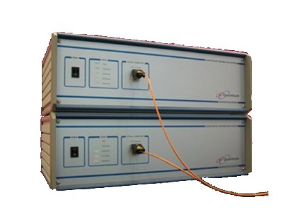
Figure 1.2: QKD today

Traditional cryptography is concerned with the secure and reliable transmission of messages. With the advent of widespread electronic communication, however, new cryptographic tasks have become increasingly important. We would like to construct secure protocols for electronic voting, online auctions, contract signing and many other applications where the protocol participants themselves do not trust each other. Two primitives that can be used to construct all such protocols are bit commitment and oblivious transfer. We will introduce both primitives in detail below. Interestingly, it turns out that despite many initially suggested protocols [BBBW82, Cré94], both primitives are impossible to achieve when we ask for unconditional security. Luckily, as we will see in Chapter 11 we can still implement both building blocks if we assume that our quantum operations are affected by noise. Here, the very problem that prevents us from implementing a full-scale quantum computer can be turned to our advantage.

In this chapter, we give an informal introduction to cryptography in the quantum setting. We first introduce necessary terminology, before giving an overview over the most well-known cryptographic primitives. Since our goal is to give an overview, we will restrict ourselves to informal definitions. Surprisingly, even definitions themselves turn out to be a tricky undertaking, especially when entering the quantum realm. Finally, we discuss what makes the quantum setting so different from the classical one, and identify a range of open problems.

1.2 Setting the state

1.2.1 Terminology

In this text, we consider protocols among multiple participants $P_{1},\ldots,P_{n}$, also called players. When considering only two players, we generally identify them with the protagonists Alice and Bob. Each player may hold a private input, that is classical and quantum data unknown to the other players. In addition, the players may have access to a shared resource such as classical shared randomness or quantum entanglement that has been distributed before the start of the protocol. We will refer to any information that is available to all players as public. A subset of players may also have access to shared information that is known only to them, but not to the remaining players. Such an input is called private shared input. In the case of shared randomness, this is also known as private shared randomness. The players can be connected by classical as well as quantum channels, and use them to exchange messages during the course of the protocol. A given protocol consists of a set of messages as well as a specification of actions to be undertaken by the players. At the end of the protocol, each player may have a classical as well as a quantum output.

A player is called honest, if he follows the protocol exactly as dictated. He is called honest-but-curious, if he follows the protocol, but nevertheless tries to gain additional information by processing the information supplied by the protocol in a way which is not intended by the protocol. An honest player, for example, will simply ignore parts of the information he is given, as he will do exactly as he is told. However, a player that is honest-but-curious will take advantage of all information he is given, i.e., he may read and copy all messages as desired, and never forgets any information he is given. Yet, the execution of the protocol itself is unaffected as the player does not change any information used in the protocol, he merely reads it. But what does this mean in a quantum setting? Indeed, this question appears to be a frequent point of debate. We will see in Chapter 2 that he cannot copy arbitrary quantum information, and extracting non-classical information from a quantum state will necessarily lead to disturbance. Evidently, disturbance alters the quantum states during the protocol. Hence, the player actually took actions to alter the execution of the protocol, and we can no longer regard him as honest. After examining quantum operations in Chapter 2 we will return to the definition of an honest-but-curious player in the quantum setting. Finally, a player can also be dishonest: he will do anything in his power to break the protocol. Evidently, this is the most realistic setting, and we will always consider it here.

An adversary is someone who is trying to break the protocol. An adversary is generally modeled as an entity outside of the protocol that can either be an eavesdropper, or take part in the protocol by taking control of specific players. This makes it easier to model protocols among multiple players, where we assume that all dishonest players collaborate to form a single adversary.

1.2.2 Assumptions

In an ideal world, we could implement any cryptographic protocol described below. Interestingly though, even in the quantum world we encounter physical limits which prevent us from doing so with unconditional security. Unconditional security most closely corresponds to the intuitive notion of “secure”. A protocol that is unconditionally secure fulfills its purpose and is secure even if an attacker is granted unlimited resources. We happily provide him with the most powerful computer we could imagine and as much memory space as he wants. The main question of unconditional security is thus whether the attacker obtains enough information to defeat the security of the system. Unconditional security is also called perfect secrecy in the context of encryption systems, and forms part of information-theoretic security.

Most often, however, unconditional security can never be achieved. We must therefore resign ourselves to introducing additional limitations on the adversary: the protocol will only be secure if certain assumptions hold. In practise, these assumptions can be divided into two big categories: In the first, we assume that the players have access to a common resource with special properties. This includes models such as a trusted initializer [Riv99], or another source that provides the players with shared randomness drawn from a fixed distribution. An example of this is also a noisy channel [CK88]: Curiously, a noisy channel that neither player can influence too much turns out to be an incredibly powerful resource. The second category consists of clear limitations on the ability of the adversary. For example, the adversary may have limited storage space available [Mau92, DFSS05], or experience noise when trying to store qubits as we will see in Chapter 11. In multi-player protocols we can also demand that dishonest players cannot communicate during the course of the protocol, that messages between different players take a certain time to be transmitted, or that only a minority of the players is dishonest. In the quantum case, other known assumptions include limiting the adversary to measure not more than a certain number of qubits at a time [Sal98], or introducing superselection rules [KMP04], where the adversary can only make a limited set of quantum measurements. When introducing such assumptions, we still speak of information-theoretic security: Except for these limitations, the adversary remains all-powerful. In particular, he has unlimited computational resources.

Classically, most forms of practical cryptography are shown to be computationally secure. In this security model, we do not grant an adversary unlimited computational resources. Instead, we are concerned with the amount of computation required to break the security of a system. We say that a system is computationally secure, if the believed level of computation necessary to defeat it exceeds the computational resources of any hypothetical adversary by a comfortable margin. The adversary is thereby allowed to use the best possible attacks against the system. Generally, the adversary is modeled as having only polynomial computational power. This means that any attacks are restricted to time and space polynomial in the size of the underlying security parameters of the system. In this setting the difficulty of defeating the system’s security is often proven to be as difficult as solving a well-known problem which is believed to be hard. The most popular problems are often number-theoretic problems such as factoring. Note that for example in the case of factoring, it is not known whether these problems are truly difficult to solve classically. Many such problems, such as factoring, fold with the advent of a quantum computer [Sho97]. It is an interesting open problem to find classical hardness assumptions, which are still secure given a quantum computer. Several proposals are known [Reg03], but so far none of them have been proven secure.

In the realm of quantum cryptography, we are so far only interested in information-theoretic security: we may introduce limitations on the adversary, but we do not resort to computational hardness assumptions.

1.2.3 Quantum properties

Quantum mechanics introduces several exciting aspects to the realm of cryptography, which we can exploit to our benefit, but which also introduce additional complications even in existing classical primitives whose security does not depend on computational hardness assumptions. Here, we give a brief introduction to some of the most striking aspects, which we will explain in detail later on.

1. Quantum states cannot be copied: In classical protocols, an adversary can always copy any messages and his classical data at will. Quantum states, however, differ: We will see in Chapter 2 that we cannot copy an arbitrary qubit. This property led to the construction of the unforgeable subway tokens [BBBW82] mentioned earlier.

2. Information gain can be detected: Classically there is no way for an honest player to determine whether messages have been read maliciously outside the scope of the protocol. However, in a quantum setting we can detect whether an adversary tried to extract information from a transmitted message. This property forms the heart of quantum key distribution described below. It also allows us to construct cheat-sensitive protocols, a concept which is foreign to classical cryptography: even though we cannot prevent an adversary from gaining information if he intends to do so, we will be able to detect such cheating and take appropriate action. We will return to this aspect in Chapter 2.

3. Uncertainty relations exist: Unlike in the classical world, quantum states allow us to encode multiple bits into a single state in such a way that we cannot extract all of them simultaneously. This property is closely related to cheat-sensitivity, and is a consequence of the existence of uncertainty relations we will encounter in Chapter 4. It is also closely related to what is known as quantum random access codes, which will we employ in Chapter 8.

4. Information can be “locked”: Another aspect we need to take into account when considering quantum protocols is an effect known as locking classical information in quantum states. Surprisingly, the amount of correlation between two parties can increase by much more than the data transmitted. We will examine this effect for a specific measure of correlation in more detail in Chapter 5.

5. Entanglement allows for stronger correlations: Entanglement is another concept absent from the classical realm. Whereas entanglement has many useful applications such as quantum teleportation and can also be used to analyze the security of quantum key distribution, it also requires us to be more cautious: In Chapter 9, we will see that the parameters of classical protocols can change dramatically if dishonest players share entanglement, even if they do not have access to a full quantum computer. In Chapter 10, entanglement will enable an adversary to break any quantum string commitment protocol.

6. Measurements can be delayed: Finally, we encounter an additional obstacle, which is also entirely missing from classical protocols: Players may delay quantum measurements. In any classical protocol, we can be assured that any input and output is fixed once the protocol ends. In the quantum case, however, players may alter their protocol input retroactively by delaying quantum measurements that depend on their respective inputs. Essentially, in a classical protocol the players will automatically be “committed” to the run of the protocol, whereas in the quantum setting this property is entirely missing. This can make an important difference in reductions among several protocols as we will see in Section 1.3.2 below.

1.3 Primitives

We now present an overview of the most common multi-party protocol primitives, and what is known about them in the quantum setting. We already encountered quantum key distribution (QKD) in the introduction. In this thesis, our focus lies on cryptographic protocols other than QKD.

1.3.1 Bit commitment

Possibly the most active area of quantum cryptography in the early stages next to QKD was quantum bit commitment: Imagine two mutually distrustful parties Alice and Bob at distant locations. They can only communicate over a channel, but want to play the following game: Alice secretly chooses a bit $c$. Bob wants to be sure that Alice indeed has made her choice. Yet, Alice wants to keep $c$ hidden from Bob until she decides to reveal $c$. To convince Bob that she made up her mind, Alice sends Bob a commitment. From the commitment alone, Bob cannot deduce $c$. At a later time, Alice reveals $c$ and enables Bob to open the commitment. Bob can now check if Alice is telling the truth. This scenario is known as bit commitment.

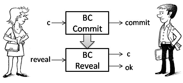
Figure 1.3: Schematic run of a BC protocol when Alice and Bob are honest.

Commitments play a central role in modern-day cryptography. They form an important building block in the construction of larger protocols in, for example, gambling and electronic voting, and other instances of secure two-party computation. In the realm of quantum mechanics, it has been shown that oblivious transfer [BBCS92b] (defined in Section 1.3.2) can be achieved provided there exists a secure bit commitment scheme [Yao95, Cré94]. In turn, classical oblivious transfer can be used to perform any secure two-party computation defined below [CvdGT95]. Commitments are also useful for constructing zero-knowledge proofs [Gol01] and lead to coin tossing [Blu83]. Informally, bit commitment can be defined as follows:

Definition 1.3.1.

Bit commitment (BC) is a two-party protocol between Alice (the committer) and Bob (the verifier), which consists of three stages, the committing and the revealing stage, and a final declaration stage in which Bob declares “accept” or “reject”. The following requirements should hold:

• (Correctness) If both Alice and Bob are honest, then before the committing stage Alice picks a bit $c$. Alice’s protocol depends on $c$ and any randomness used. At the revealing stage, Alice reveals to Bob the committed bit $c$. Bob accepts.

• (Binding) If Alice wants to reveal a bit $c^{\prime}$, then

  $$\Pr[\mbox{Bob accepts }|c^{\prime}=0]+\Pr[\mbox{Bob accepts }|c^{\prime}=1]\leq 1.$$

• (Concealing) If Alice is honest, Bob does not learn anything about $c$ before the revealing stage.

Classically, unconditionally secure bit commitment is known to be impossible. Indeed, this is very intuitive if we consider the implications of the concealing condition: This condition implies that exactly the same information exchange must have occurred if Alice committed herself to $c=0$ or $c=1$, otherwise Bob would be able to gain information about $c$. But this means that even if Alice initially made a commitment to $c=0$, she can later reconstruct the run of the protocol as if she had committed herself to $c=1$ and thus send the right message to Bob to reveal $c=1$ instead. Unfortunately, even quantum communication cannot help us to implement unconditionally secure bit commitment without further assumptions: After several quantum schemes were suggested [BB84, BC90a, BCJL93], quantum bit commitment was shown to be impossible, too [May96b, LC97, May97, LC96, BCMS97, CL98, DKSW06], even in the presence of superselection rules [KMP04], where the adversary can only perform a certain restricted set of measurements. In the face of the negative results, what can we still hope to achieve?

Evidently, we need to assume that the adversary is limited in certain ways. In the classical case, bit commitment is possible if the adversary is computationally bounded [Gol01], if one-way functions exist [Nao91, HR07], if Alice and Bob are connected via a noisy channel that neither player can influence too much [CK88, DKS99, DFMS04], or if the adversary is bounded in space instead of time, i.e., he is only allowed to use a certain amount of storage space [Mau92]. Unfortunately, the security of the bounded classical storage model [Mau92, CCM98] is somewhat unsatisfactory: First, a dishonest player needs only quadratically more memory than the honest one to break the security. Second, as classical memory is very cheap, most of these protocols require huge amounts of communication in order to achieve reasonable bounds on the adversaries memory.

Do we gain anything by using quantum communication? Interestingly, even without any further assumptions, quantum cryptography at least allows us to implement imperfect forms of bit commitment, where Alice and Bob both have a limited ability to cheat. That is, we allow Alice to change her mind, and Bob to learn the committed bit with a small probability. These protocols are based on the fact that quantum protocols can exhibit a form of cheat sensitivity unavailable to classical communication [HK04, ATSVY00]. Exact tradeoffs on how well we can implement bit commitment in the quantum world can be found in [SR02a]. Protocols that make use of this tradeoff are cheat-sensitive, as described in Section 1.2.2. Examples of such protocols have been used to implement coin tossing [Amb01] as described in Section 1.3.2. In Chapter 10, we will consider commitments to an entire string of bits at once. Whereas this task turns out to be impossible as well for a strong security definition, we will see that non-trivial quantum protocols do exist for a very weak security definition. Bit commitment can also be implemented under the assumption that faster than light communication is impossible, provided that Alice and Bob are located very far apart [Ken99], or if Alice and Bob are given access to non-local boxes [BCU⁺06] which provide superstrong non-local correlations.

But even a perfect commitment can be implemented, if we make quantum specific assumptions. For example, it is possible to securely implement BC provided that an adversary cannot measure more than a fixed number of qubits simultaneously [Sal98]. With current-day technology, it is very difficult to store states even for a very short period of time. This leads to the protocol presented in [BBCS92a, Cré94], which shows how to implement BC and OT (defined below) if the adversary is not able to store any qubits at all. In [DFSS05, DFR⁺07], these ideas have been generalized in a very nice way to the bounded-quantum-storage model, where the adversary is computationally unbounded and is allowed to have an unlimited amount of classical memory. However, he is only allowed a limited amount of quantum memory. The advantages over the classical bounded-storage model are two-fold: First, given current day technology it is indeed very hard to store quantum states. Secondly, the honest players do not require any quantum storage at all, making the protocol much more efficient. It has been shown that such protocols remain secure when executed many times in a row [WW07].

1.3.2 Secure function evaluation

An important aspect of modern day cryptography is the primitive known as secure function evaluation, and its multi-player analogue, secure multi-party computation, first suggested by Yao [Yao82]. Imagine that Alice and Bob are trying to decide whether to attend an unpopular administrative event. If Alice attends, Bob feels forced to attend as well and vice versa. However, neither of them wants to announce publicly whether they are planning to attend or whether they would rather make up an excuse to remain at home, as this may have dire consequences. How can Alice and Bob solve their dilemma? Note that their problem can be phrased in the following form: Let $x$ be Alice’s private input bit, where $x=1$ if Alice is planning to attend and $x=0$ if Alice skips the event. Similarly, let $y$ be Bob’s private input bit. Alice and Bob now want to compute $\mbox{OR}(x,y)$ in such a way that both of them learn the result, but neither of them learns anything more about the input of the other player than can be inferred from the result. In our example, if $\mbox{OR}(x,y)=1$, at least one of the players is planning to attend the event. Both Alice and Bob now attend the event, and both of them can safely claim that they really did plan to do so in the first place. If $\mbox{OR}(x,y)=0$, Alice and Bob learn that they both agree, and do not need to fear any political consequences.

Secure function evaluation enables Alice and Bob to solve any such task. Protocols for secure function evaluation enable us to construct protocols for electronic voting and secure auctions. Informally, we define:

Definition 1.3.2.

Secure function evaluation (SFE) is a two-party protocol between Alice and Bob, where Alice holds a private input $x$ and Bob holds a private input $y$ such that

• (Correctness) If both Alice and Bob are honest, then they both output the same value $v=f(x,y)$.

• (Security) If Alice (Bob) is dishonest, then Alice (Bob) does not learn more about $x$ ($y$) then can be inferred from $f(x,y)$.

A common variant of SFE is so-called one-sided SFE: Here, only one of the two players receives the result of the computation, $f(x,y)$. Sadly, we cannot implement SFE for an arbitrary function $f$ classically without additional assumptions, akin to bit commitment. Even in the quantum world, the situation is equally bleak: SFE remains impossible in the quantum setting [Lo97]! Fortunately, the situations improves when we consider multi-party protocols as mentioned below.

Oblivious transfer

A special case of secure function evaluation is the problem of oblivious transfer, which was first introduced by Rabin [Rab81]. The variant of 1-2 OT appeared in a paper by Even, Goldreich and Lempel [EGL85] and also, under a different name, in the well-known paper by Wiesner [Wie83]. 1-2 OT allows Alice and Bob to solve a seemingly uninteresting problem: The sender (Alice) secretly chooses two bits $s_{0}$ and $s_{1}$, the receiver (Bob) secretly chooses a bit $c$. The primitive of oblivious transfer allows Bob to retrieve $s_{c}$ in such a way, that Alice cannot gain any information about $c$. At the same time, Alice is ensured that Bob only retrieves $s_{c}$ and gets no information about the other input bit $s_{\bar{c}}$. Oblivious transfer can be used to perform any secure two-party computation [Kil88, CvdGT95], and is therefore a very important primitive.

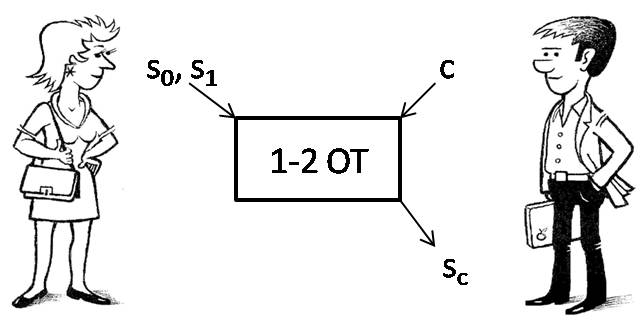
Figure 1.4: Schematic run of a 1-2 OT protocol.

Unlike in the classical setting, oblivious transfer in the quantum world requires additional caution: We want that after the protocol ends, both of Alice’s inputs bits $s_{0},s_{1}$ and Bob’s choice bit $c$ have been determined. That is, they are fixed and the players can no longer change their mind. In particular, we do not want Bob to delay his choice of $c$ indefinitely, possibly by delaying a quantum measurement. Similarly, Alice should not be able to change her mind about, for example, the parity of $s_{0}\oplus s_{1}$ after the end of the protocol by delaying a measurement. Informally, we define

Definition 1.3.3.

${2\choose 1}$-oblivious transfer (1-2 OT$(s_{0},s_{1})(c)$) is a two-party protocol between Alice (the sender) and Bob (the receiver), such that

• (Correctness) If both Alice and Bob are honest, the protocol depends on Alice’s two input bits $s_{0},s_{1}\in\{0,1\}$ and Bob’s input bit $c\in\{0,1\}$. At the end of the protocol Bob knows $s_{c}$.

• (Security against Alice) If Bob is honest, Alice does not learn $c$.

• (Security against Bob) If Alice is honest, Bob does not learn anything about $s_{\bar{c}}$.

After the protocol ends, $s_{0},s_{1}$ and $c$ have been chosen.

Classically, 1-2 OT can be obtained from the following simpler primitive, also known as Rabin-OT [Rab81] or erasure channel. Conversely, OT can be obtained from 1-2 OT.

Definition 1.3.4.

Rabin Oblivious transfer (Rabin-OT) is a two-party protocol between Alice (the sender) and Bob (the receiver), such that

• (Correctness) If both Alice and Bob are honest, the protocol depends on Alice’s input bit $b\in\{0,1\}$. At the end of the protocol, Bob obtains $b$ with probability $1/2$ and knows whether he obtained $b$ or not.

• (Security against Alice) If Bob is honest, Alice does not learn whether Bob obtained $b$.

• (Security against Bob) If Alice is honest, Bob’s probability of learning bit $b$ does not exceed $1/2$.

After the protocol ends, $b$ has been chosen.

The fact that Alice and Bob may delay their measurements makes an important difference, as the following simple example shows: Consider the standard reduction of Rabin-OT to 1-2 OT: Alice uses inputs $s_{k}=b$ and $s_{\bar{k}}=0$ with $k\in_{R}\{0,1\}$. Bob uses input $c\in_{R}\{0,1\}$, for a randomly chosen $c$. The players now perform 1-2 OT$(s_{0},s_{1})(c)$ after which the receiver holds $s_{c}$. Subsequently, Alice announces $k$. If $k=c$, Bob succeeded in retrieving $b$ and otherwise he learns nothing. This happens with probability $p=1/2$ and thus we have constructed Rabin-OT from one instance of 1-2 OT. Clearly, this reduction fails if we use an 1-2 OT protocol in which Bob can defer his choice of $c$, possibly by delaying a quantum measurement that depends on $c$. He simply waits until Alice announces $k$, to retrieve $s_{k}$ with certainty. This simple example makes it clear that implementing 1-2 OT is far from a trivial task in the quantum setting. Even the classical definitions need to be revised carefully. In this brief overview, we restricted ourselves to the informal definition given above, and refer to [Wul07] for an extensive treatment of the definition of oblivious transfer.

Note that oblivious transfer forms an instance of secure function evaluation with $f:\{0,1\}^{2}\times\{0,1\}\rightarrow\{0,1\}$ satisfying $f(s_{0},s_{1},c)=s_{c}$, where only one player (Bob) learns the output. Hence by Lo’s impossibility result for SFE discussed earlier, oblivious transfer is not possible in the quantum setting either without introducing additional assumptions. Indeed, note that there exists a classical reduction of bit commitment to oblivious transfer (up to a vanishing probability), where we reverse the roles of Alice and Bob for bit commitment: Alice simply chooses two $n$-bit strings $x_{0}\in_{R}\{0,1\}^{n}$, and $x_{1}\in_{R}\{0,1\}^{n}$. Alice and Bob now use $n$ rounds of 1-2 OT, where Bob retrieves $x_{c}$ when he wants to commit to a bit $c$. To reveal, he then sends $c$ and $x_{c}$ to Alice. Intuitively, one can thus hope to use the impossibility proof of bit commitment to show that oblivious transfer is impossible as well, without resorting to [Lo97]. However, note that we would first have to show the security of this reduction with respect to a quantum adversary. Fortunately, oblivious transfer becomes possible if we make the same assumptions as for bit commitment described in Section 1.3.1. We will consider how to implement oblivious transfer if the adversary’s quantum storage is subject to noise in Chapter 11.

Coin tossing

Another example of SFE is the well-known primitive of coin tossing [Blu83], which can be viewed as an instance of randomized secure function evaluation defined in [Gol01]. Imagine that Alice and Bob want to toss a coin, solely by communicating over a classical and a quantum channel. We thereby want to ensure that neither party can influence the outcome of the coin toss by too much. Unfortunately, we cannot implement this primitive classically without relying on additional assumptions.

What assumptions do we need to implement coin tossing? It is easy to see that we can implement one form of coin tossing, if we could perform bit commitment: Alice chooses a random bit $b\in_{R}\{0,1\}$ and commits herself to $b$. Subsequently, Bob chooses a random bit $b^{\prime}\in_{R}\{0,1\}$ and sends it to Alice. After receiving $b^{\prime}$, Alice opens her commitment and reveals $b$. Both parties now output $c=b\oplus b^{\prime}$ as their outcome. Thus, any assumptions that enable us to implement bit commitment also lead to coin tossing. Some assumptions even allow for very simple protocols: If we assume that Alice and Bob are located far apart and faster-than-light communication is impossible, they can simply both flip a coin themselves and send it over the channel. They then take the xor of the two bits as the outcome of the coin flip. If Alice and Bob do not receive the other’s bit within a certain time frame they reject this execution of the protocol and restart. Since it takes the bit a specific time to travel over the channel, both parties can be sure that it must have been sent before a certain time, i.e., before receiving the other’s bit.

Many definitions of coin tossing are known in the literature, which exhibit subtle differences especially whether aborts are allowed during the protocol. In the quantum literature, strong coin tossing has been informally defined as follows:

Definition 1.3.5.

A quantum strong coin tossing protocol with bias $\varepsilon$ is a two-party protocol, where Alice and Bob communicate and finally decide on a value $c\in\{0,1,\perp\}$ such that

• If both parties are honest, then $\Pr[c=0]=\Pr[c=1]=1/2$.

• If one party is honest, then for any strategy of the dishonest player $\Pr[c=0]\leq 1/2+\varepsilon$ and $\Pr[c=1]\leq 1/2+\varepsilon$.

Sadly, strong coin tossing cannot be implemented perfectly with bias $\varepsilon=0$ [LC98]. However, one might hope that one could still achieve an arbitrarily small bias $\varepsilon>0$. Many protocols have been proposed for quantum strong coin tossing and subsequently been broken [MSC99, ZLG00]. Sadly, it was shown that strong coin tossing cannot be implemented with an arbitrarily small bias, and $\varepsilon=1/\sqrt{2}-1/2\approx 0.207$ is the best we could hope to achieve [Kit02]. So far, quantum protocols for strong coin tossing with a bias of $\varepsilon\approx 0.42$ [ATSVY00] and finally $\varepsilon=1/4$ [Amb01, SR02a, KN04, Col07] are known. No formal definition of strong coin tossing in the quantum setting is known to date, that specifies how to deal with an abort in the case when the protocol is executed multiple times.

To circumvent this problem, a slightly weaker primitive has been proposed, which carries the name weak coin tossing in the quantum literature. Here, we explicitly allow the dishonest party to bias the coin entirely in one direction, but limit his ability to bias the coin the other way. This scenario corresponds to a setting where, for example, Alice wins if the outcome is $c=0$ and Bob if $c=1$. However, we do allow each player to give in and loose at will. Intuitively, this setting makes more sense in all common practical examples when considering a standalone run of such a protocol, where each player has a preferred outcome. Informally, we define

Definition 1.3.6.

A quantum weak coin tossing protocol with bias $\varepsilon$ is a two-party protocol, where Alice and Bob communicate and finally decide on a value $c\in\{0,1,\perp\}$ such that

• If both parties are honest, then $\Pr[c=0]=\Pr[c=1]=1/2$.

• If Alice is honest, then for any strategy of Bob

  $$\Pr[c=1]\leq 1/2+\varepsilon.$$

• If Bob is honest, then for any strategy of Alice

  $$\Pr[c=0]\leq 1/2+\varepsilon.$$

Weakening the definition in this way indeed helps us! It has been shown that we can construct a quantum protocol for weak coin tossing that achieves a bias of $\varepsilon\approx 0.239$ [KN04], $\varepsilon\approx 0.207$ [SR02b], $\varepsilon\approx 0.192$ [Moc04], and $\varepsilon\approx 0.167$ [Moc05]. Very recently, however, a protocol with an arbitrarily small bias has been suggested [Moc07b]! To date, there is also no formal definition of weak coin tossing in the quantum setting.

Multiple players

Secure multi-party computation (SMP) concerns an analogous task to SFE, involving $n$ players $P_{1},\ldots,P_{n}$, where $P_{j}$ has a private input $x_{j}$. Their goal is to compute $f(x_{1},\ldots,x_{n})$, such that none of them can learn more about the input of any other player than they can infer from $f(x_{1},\ldots,x_{n}$). Fortunately, the situation changes dramatically when extending the protocol to multiple players. SMP can be implemented with unconditional security even classically, provided that $t<n/3$ of the players are dishonest [Gol01]. If the adversary is not dishonest, but merely honest-but-curious, it is possible to increase $t$ up to $t<n/2$ [Gol01]. We refer to [Cra99] for an overview of classical secure multi-party computation.

Quantumly, one can generalize secure multi-party computation to the following setting. Each player $P_{j}$ holds an input state $\rho_{i}\in\mathcal{H}$ (see Chapter 2 for details). Let $\rho\in\mathcal{H}_{1}\otimes\ldots\otimes\mathcal{H}_{n}$ denote the joint state of players $P_{1},\ldots,P_{n}$. Then quantum secure multi-party computation (QSMP) allows the players to compute any quantum transformation $U$ to obtain $U\rho U^{\dagger}$, where player $P_{j}$ receives the quantum state on $\mathcal{H}_{j}$ as his output. QSMP can be implemented securely if $t<n/2$ of the players are dishonest [CGS02, CGS05].

Coin tossing has also been studied in the multi-party setting. Classically, multi-party coin tossing forms part of secure multi-party computation [Gol01], and can thus be implemented under the same assumptions. Quantumly, multi-party coin tossing has been studied in [ABRD04].

1.3.3 Secret sharing

Another interesting problem concerns the sharing of a classical or quantum secret. Imagine Alice holding an important piece of information, for example the launch code to her personal missile silo. Alice would like to enable members of her community to gain access, but wants to prevent a single individual from launching a missile on his own. Secret sharing enables Alice to distribute some secret data $d$ among a set of $n$ players, such that at least $t>1$ players need to combine their individual shares to reconstruct the original secret $d$. A trivial secret sharing scheme for a bit $d\in\{0,1\}$ involving just two players is as follows: Alice picks $r\in_{R}\{0,1\}$ and hands $s_{1}=d\oplus r$ to the first player, and $s_{2}=r$ to the second player. Clearly, if $r$ is chosen uniformly at random from $\{0,1\}$, none of the individual players can gain any information about $d$. Yet, when combining their individual shares they can compute $s_{1}\oplus s_{2}=d$.

General secret-sharing schemes were introduced by Shamir [Sha79] and Blakey [Bla79]. They have found a wide range of applications, most notably to construct protocols for secure multi-party computation as described in Section 1.3.2. Many classical secret sharing schemes are known today [MvOV97]. Quantum secret sharing was first introduced in [HBB99] and shortly after in [CGL99], which also formed a link between quantum secret sharing schemes and error correcting codes. Quantumly, we can distinguish two types of secret sharing schemes: The first allows to share a quantum secret, i.e., Alice holds a quantum state $\rho$ and wants to construct $n$ quantum shares $\sigma_{1},\ldots,\sigma_{n}$ such that when $t$ such shares are combined $\rho$ can be reconstructed [HBB99, CGL99, Got00]. The second allows us to share classical secrets using quantum states that have very nice data-hiding properties [DLT02, DHT03, EW02, HLS05]: it is not sufficient for $n$ parties to perform local measurements and communicate classically in order to reconstruct the secret. To reconstruct the secret data they must communicate quantumly to perform a coherent measurement on their states. It is an exciting open question whether such schemes can be used to implement quantum protocols for secure multi-party computations with classical inputs that remain secure as long as the dishonest players can only communicate classically, but not quantumly.

1.3.4 Anonymous transmissions

In all applications we considered so far, we were concerned with two aspects: either, we wanted to protect protocol participants from being cheated by the other players, or, we wanted to protect the secrecy of data from a third party as in the setting of key distribution described in Section 1.1. In the problem of key distribution, sender and receiver know each other, but are trying to protect their data exchange from prying eyes. Anonymity, however, is the secrecy of identity. Primitives to hide the sender and receiver of a transmission have received considerable attention in classical computing. Such primitives allow any member of a group to send and receive data anonymously, even if all transmissions can be monitored. They play an important role in protocols for electronic auctions [SA99], voting protocols and sending anonymous email [Cha81]. An anonymous channel which is completely immune to any active attacks, would be a powerful primitive. It has been shown how two parties can use such a channel to perform key-exchange [AS83].

A considerable number of classical schemes have been suggested for anonymous transmissions. An unconditionally secure classical protocol was introduced by Chaum [Cha88] in the context of the Dining Cryptographers Problem. Such a protocol can also be considered an instance of secure multi-party computation considered above.

Boykin [Boy02] considered a quantum protocol to send classical information anonymously where the players distribute and test pairwise shared EPR pairs, which they then use to obtain key bits. His protocol is secure in the presence of noise or attacks on the quantum channel. In [CW05a], we presented a protocol for anonymous transmissions of classical data that achieves a novel property that cannot be achieved classically: it is completely traceless. This property is related, but stronger than the notion of incoercibility in secure multi-party protocols [CG96]. Informally, a protocol is traceless, if a player cannot be forced to reveal his true input at the end of the protocol. Even when forced to hand out his input, output and randomness used during the course of the protocol, a player is able to generate fake input that is consistent with all other data gathered from the run of the protocol. The protocols suggested in [Boy02] are not traceless, but can be modified to exhibit this property. It would be interesting to see whether it is possible to make general protocols for secure multi-party computation similarly traceless.

The first protocol for the anonymous transmission of qubits was constructed in [CW05a]. Whereas the anonymous transmissions of classical bits can be implemented via secure multi-party computation, the scenario is different when we wish to transmit qubits: as we will see in Chapter 2, qubits cannot be copied. Thus we cannot expect each player to obtain a copy of the output. New protocols for creating anonymous entanglement and anonymously transmitting qubits have since been suggested in [BS05, BBF⁺].

1.3.5 Other protocols

Besides the protocols above, a variety of other primitives making use of particular quantum effects have been proposed. One of the oldest suggested applications is the one of quantum money that is resistant to copying [Wie83], also proposed as unforgeable subway tokens [BBBW82]. Quantum seals [BP03, Cha03, SS05] employ the notion of cheat sensitivity in order to provide data with a seal that is “broken” once the data is extracted. That is, we can detect whether the data has been read. Perfect quantum seals that allow us to detect tampering with certainty have been shown to be impossible [BPDM05]. Nevertheless, non-trivial constructions are can be implemented.

Furthermore, quantum signature schemes [GC01] have been proposed which exhibit unconditional security: here Bob can verify Alice’s signature using a public key given to him ahead of time. Sadly, such a scheme slowly consumes the necessary public key. Finally, protocols have been suggested for the encryption of quantum data which allow $n$ qubits to be encoded using a $2n$ bit key achieving perfect secrecy [BR03, AMTdW00]. Much smaller keys are possible, if we allow for small imperfections [DN06, AS04]. Such encryption schemes have also been used to allow for private circuit evaluation [Chi05]: Here, Alice encrypts her quantum state before handing it to Bob who is capable of running a certain quantum operation that Alice would like to apply. This allows Alice to let her quantum operations be performed by Bob without revealing her quantum input.

1.4 Challenges

As we saw in Section 1.2.3, introducing quantum elements into cryptography leads to interesting new effects. Much progress has been made to exploit these quantum effects, although many open questions remain. In particular, not much is known about how well quantum protocols compose. That is, when we use one protocol as a building block inside a larger application, does the protocol still remain secure as expected? Recall from Section 1.2.3 that especially our ability to delay quantum measurements has a great influence on composition. Fortunately, quantum key distribution has been shown composable [BOHL⁺05, Ren05, RK05]. However, composability remains a particularly tricky question in protocols where we are not faced with an external eavesdropper, but where the players themselves are dishonest. Composability of quantum protocols was first considered in [vdG98], followed by [CGS02] who addressed the composability of QSMP, and the general composability frameworks of [Unr04, BOM04] applied to QKD [BOHL⁺05]. Great care must also be taken when composing quantum protocols in the bounded quantum storage model [WW07]. Even though these composability frameworks exist, very few protocols have been proven secure when composed.

Secondly, we need to consider what happens if an adversary is allowed to store even small amounts of quantum information. There are many examples known where quantum memory can prove much more useful to an adversary than classical memory [GKK⁺06], and we will encounter such examples in Chapters 3 and 5.

Furthermore, it is often assumed that the downfall of computational assumptions such as factoring is the only consequence that quantum computing has on the security of classical protocols. Sadly, this is by no means the only problem. Classical protocols where the security depends on the fact that different players cannot communicate during the course of the protocol may be broken when the players can share quantum entanglement and perform even a very limited set of quantum operations, well within the reach of current day technology. We will encounter such an example in Chapter 9.

Furthermore, we may conceive new primitives, unknown to the classical setting. One such primitive is the distribution of shared quantum states in the presence of dishonest players. Here, our goal is to create a protocol among $n$ players such that at the end of the protocol $m\leq n$ players share a specified state $\rho$, where the dishonest players may apply any measurement to their share. It is conceivable to extend the QSMP protocol of [CGS02] to address this problem, yet, much more efficient protocols may be possible. Such a primitive would also enable us to build up the resources needed by other protocols such as [CW05a].

Finally, it is an interesting question by itself, what cryptographic primitives are possible in a quantum mechanical world. Conversely, it has even been shown that the axioms governing quantum mechanics can in part be obtained from the premise that perfect bit commitment is impossible [CBH03]. Perhaps such connections may lead to novel insights.

1.5 Conclusion

Quantum cryptography beyond quantum key distribution is an exciting subject. In this thesis, we will investigate several aspects that play an important role in nearly all cryptographic applications in the quantum setting.

In part I, we will examine how to extract information from quantum states. We first consider the problem of state discrimination. Here, our goal is to determine the identity of a state $\rho$ within a finite set of possible states $\{\rho_{1},\ldots,\rho_{n}\}$. In Chapter 3, we will examine a special case of this problem that is of particular relevance to quantum cryptography in the bounded quantum storage model: How well can we perform state discrimination if we are given additional information after an initial quantum measurement, i.e., after a quantum memory bound is applied? In Chapter 4, we address uncertainty relations, which play an important role in nearly all cryptographic applications. We will prove tight bounds for uncertainty relations for certain mutually unbiased measurements. We will also present optimal uncertainty relations for anti-commuting measurements. Finally, in Chapter 5, we then examine a peculiar quantum effect known as locking classical information in quantum states. Such effects are important in the security of QKD, and also play a role in quantum string commitments which we will encounter in part III. In particular, we address the following question: Can we always obtain good locking effects for mutually unbiased measurements?

In part II, we turn to investigate quantum entanglement. In Chapter 7, we show how to find optimal quantum strategies for two parties who cannot communicate, but share quantum entanglement. Understanding such strategies plays an important part in understanding the effect of entanglement in otherwise classical protocols. In Chapter 8, we then present some initial weak result on the amount of entanglement such strategies require. Finally, in Chapter 9, we show how the security of classical protocols can be affected considerably in the presence of entanglement.

In part III, we investigate two cryptographic problems directly. In Chapter 10, we first consider commitments: Quantumly, one may hope that committing to an entire string of bits at once, and allowing Alice and Bob a limited ability to cheat, may still be within the realm of possibilities. This does not contradict that bit commitment itself is impossible. Unfortunately, we will see that for any reasonable security measure, string commitments are also impossible. However, non-trivial protocols do become possible for very weak notions of security.

In Chapter 11, we then introduce the model of noisy-quantum storage that in spirit is very similar to the setting of bounded-quantum storage: Here we assume that the adversary’s quantum operations and storage are subject to noise. We show that oblivious transfer can be implemented securely in this model. We give an explicit tradeoff between the amount of noise and the security of our protocol.

Part II Information in quantum states

Chapter 2 Introduction

To investigate the limitations and possibilities of cryptographic protocols in a physical world, we must familiarize ourselves with its physical theory: quantum mechanics. What are quantum states and what sets them apart from the classical scenario? Here, we briefly recount the most elementary facts that will be necessary for the remainder of this text. We refer to [Per93] for a more gentle introduction to quantum mechanics, to Appendix A for linear algebra prerequisites, and to the symbol index on page IV for unfamiliar notation. In later chapters, we examine some of the most striking aspects of quantum mechanics, such as uncertainty relations and entanglement in more detail.

2.1 Quantum mechanics

2.1.1 Quantum states

A $d$-dimensional quantum state is a positive semidefinite operator $\rho$ of norm 1 (i.e., $\rho$ has no negative eigenvalues and $\mbox{\rm Tr}(\rho)=1$) living in a $d$-dimensional Hilbert space $\mathcal{H}$. We commonly refer to $\rho$ as a density operator or density matrix. A special case of a quantum state is a pure state, which has the property that $\mbox{rank}(\rho)=1$. That is, there exists some vector $|\Psi\rangle\in\mathcal{H}$ such that we can write $\rho=|\Psi\rangle\langle\Psi|$, where $|\Psi\rangle\langle\Psi|$ is a projector onto the vector $|\Psi\rangle$. If $\{|0\rangle,\ldots,|d-1\rangle\}$ is a basis for $\mathcal{H}$, we can thus write $|\Psi\rangle=\sum_{j=0}^{d-1}\alpha_{j}|j\rangle$ for some coefficients $\alpha_{j}\in\mathbb{C}$. Note that our normalization constraint implies that $\mbox{\rm Tr}(\rho)=\sum_{j}|\alpha_{j}|^{2}=1$. We also say that $|\Psi\rangle$ is in a superposition of vectors $|0\rangle,\ldots,|d-1\rangle$. Clearly, for a pure state we have that $\rho^{2}=\rho$ and thus $\mbox{\rm Tr}(\rho^{2})=1$.

Let’s first look at an example of pure states. Suppose we consider a $d=2$ dimensional quantum system $\mathcal{H}$, also called a qubit. We call $\{|0\rangle,|1\rangle\}$ the computational basis, where

$$|0\rangle=\left(\begin{array}[]{c}1\\ 0\end{array}\right)\mbox{ and }|1\rangle=\left(\begin{array}[]{c}0\\ 1\end{array}\right).$$

Any pure qubit state can then be written as $|\Psi\rangle=\alpha|0\rangle+\beta|1\rangle$ for some $\alpha,\beta\in\mathbb{C}$ with $|\alpha|^{2}+|\beta|^{2}=1$. We take an encoding of ’0’ or ’1’ in the computational basis to be $|0\rangle$ or $|1\rangle$ respectively, and use the subscript ’+’ to refer to an encoding in the computational basis. An alternative choice of basis would be the Hadamard basis, given by vectors $\{|+\rangle,|-\rangle\}$, where

$$|+\rangle=\frac{1}{\sqrt{2}}(|0\rangle+|1\rangle)\mbox{ and }|-\rangle=\frac{1}{\sqrt{2}}(|0\rangle-|1\rangle).$$

We use ’$\times$’ to refer to an encoding in the Hadamard basis. We will often consider systems consisting of $n$ qubits. If $\mathcal{H}$ is a 2-dimensional Hilbert space corresponding to a single qubit, the system of $n$ qubits is given by the $n$-fold tensor product $\mathcal{H}^{\otimes n}$ with dimension $d=2^{n}$. A basis for this larger Hilbert space can easily be found by forming the tensor products of the basis vectors of a single qubit. For example, the computational basis for an $n$-qubit system is given by the basis vectors $\{|x_{1}\rangle\otimes\ldots\otimes|x_{n}\rangle\mid x_{j}\in\{0,1\},j\in[n]\}$ where $[n]=\{1,\ldots,n\}$. We will often omit the tensor product and use the shorthand $|x_{1}\ldots x_{n}\rangle=|x_{1}\rangle\otimes\ldots\otimes|x_{n}\rangle$.

If $\rho$ is not pure, then $\rho$ is a mixed state and can be written as a mixture of pure states. That is, for any state $\rho$ there exist $\lambda_{j}\geq 0$ with $\sum_{j}\lambda_{j}=1$ and vectors $|\Psi_{j}\rangle$ such that

$$\rho=\sum_{j}\lambda_{j}|\Psi_{j}\rangle\langle\Psi_{j}|.$$

Since $\rho$ is Hermitian, we can take $\lambda_{j}$ and $|\Psi_{j}\rangle$ to be the eigenvalues and eigenvectors of $\rho$ respectively. We thus have for any quantum state that $\mbox{\rm Tr}(\rho^{2})\leq 1$, where equality holds if and only if $\rho$ is a pure state. We can also consider a mixture of quantum states, pure or mixed. Suppose we have a physical system whose state $\rho_{x}$ depends on some value $x\in\mathcal{X}$ of a classical random variable $X$ drawn from $\mathcal{X}$ according to a probability distribution $P_{X}$. For anyone who does not know the value of $X$ (but does know the distribution $P_{X}$), the state of the system is given as

$$\rho=\sum_{x}P_{X}(x)\rho_{x}.$$

We also call the set $\mathcal{E}=\{(P_{X}(x),\rho_{x})\mid x\in\mathcal{X}\}$ an ensemble, that gives rise to the density matrix $\rho$. We generally use the common shorthand $\mathcal{E}=\{P_{X}(x),\rho_{x}\}$. Clearly, for any state $\rho$ we can take its eigendecomposition as above to find one possible ensemble that gives rise to $\rho$. With this interpretation in mind, it is now intuitive why we wanted $\rho\geq 0$ and $\mbox{\rm Tr}(\rho)=1$: the first condition ensures that $\rho$ has no negative eigenvalues and hence all probabilities $\lambda_{j}$ are non-negative. The second condition ensures that the resulting distribution in indeed normalized. We will use $\mathcal{S}(\mathcal{H})$ and $\mathbb{B}(\mathcal{H})$ to denote the set of all density matrices and the set of all bounded operators on a system $\mathcal{H}$ respectively.

Let’s look at a small example illustrating the concept of mixed quantum states. The density matrices corresponding to $|0\rangle$ and $|1\rangle$ are $\rho_{0+}=|0\rangle\langle 0|$ and $\rho_{1+}=|1\rangle\langle 1|$, and the density matrices corresponding to $|+\rangle$ and $|-\rangle$ are given by $\rho_{0\times}=|+\rangle\langle+|$ and $\rho_{1\times}=|-\rangle\langle-|$. Let’s suppose we are now told that we are given a ’0’ but encoded in either the computational or Hadamard basis, each with probability $1/2$. Our quantum state corresponding to this encoding of ’0’ is now

$$\rho_{0}=\frac{1}{2}(\rho_{0+}+\rho_{0\times}).$$

The state corresponding to an encoding of ’1’ is similarly given by

$$\rho_{1}=\frac{1}{2}(\rho_{1+}+\rho_{1\times}).$$

It is important to note that the same density matrix can be generated by two different ensembles. As a simple example, consider the matrix $\rho=(2/3)|0\rangle\langle 0|+(1/3)|1\rangle\langle 1|$. Clearly, $\rho\geq 0$ and $\mbox{\rm Tr}(\rho)=1$ and thus $\rho$ forms a valid one qubit quantum state. However, $\mathcal{E}_{1}=\{(2/3,|0\rangle),(1/3,|1\rangle)\}$ and $\mathcal{E}_{2}=\{(1/2,|\phi_{0}\rangle),(1/2,|\phi_{1}\rangle)\}$ with $|\phi_{0}\rangle=\sqrt{2/3}|0\rangle+\sqrt{1/3}|1\rangle$ and $|\phi_{1}\rangle=\sqrt{2/3}|0\rangle-\sqrt{1/3}|1\rangle$ both give rise to $\rho$:

$$\rho=\frac{2}{3}|0\rangle\langle 0|+\frac{1}{3}|1\rangle\langle 1|=\frac{1}{2}|\phi_{0}\rangle\langle\phi_{0}|+\frac{1}{2}|\phi_{1}\rangle\langle\phi_{1}|.$$

Classical vs. Quantum
Quantum states exhibit an important property known as “no-cloning”: very much unlike classical states, we cannot create a copy of an arbitrary quantum state! This is only possible with a small probability. We refer to [SIGA05] for an excellent overview of known results.

In the following, we call an ensemble classical if all states $\rho_{x}$ commute. This is an interesting special case, we discuss in more detail below.

2.1.2 Multipartite systems

We frequently need to talk about a quantum state shared by multiple players in a protocol. Let $\mathcal{H}_{1},\ldots,\mathcal{H}_{n}$ denote the Hilbert spaces corresponding to the quantum systems of players 1 up to $n$. As outlined in the case of multiple qubits above, the joint system $\mathcal{H}_{1}\otimes\ldots\otimes\mathcal{H}_{n}$ of all players is formed by taking the tensor product. For example, suppose that we have only two players, Alice and Bob. Let $\mathcal{H}^{A}$ and $\mathcal{H}^{B}$ be the Hilbert spaces corresponding to Alice’s and Bob’s quantum systems respectively. Any bipartite state $\rho^{AB}$ shared by Alice and Bob is a state living in the joint system $\mathcal{H}^{A}\otimes\mathcal{H}^{B}$. Bipartite states can exhibit an interesting property called entanglement, which we investigate in Chapter 6. In short, if $|\Psi\rangle\in\mathcal{H}^{A}\otimes\mathcal{H}^{B}$ is a pure state, we say that $|\Psi\rangle$ is separable if and only if there exist states $|\Psi^{A}\rangle\in\mathcal{H}^{A}$ and $|\Psi^{B}\rangle\in\mathcal{H}^{B}$ such that $|\Psi\rangle=|\Psi^{A}\rangle\otimes|\Psi^{B}\rangle$. A separable pure state is also called a product state. A state that is not separable is called entangled. An example of an entangled pure state is the so-called EPR-pair

$$\frac{1}{2}(|00\rangle+|11\rangle).$$

For mixed states the definition is slightly more subtle. Let $\rho\in\mathcal{S}(\mathcal{H}^{A}\otimes\mathcal{H}^{B})$ be a mixed state. Then $\rho$ is called a product state if there exist $\rho^{A}\in\mathcal{H}^{A}$ and $\rho^{B}\in\mathcal{H}^{B}$ such that $\rho=\rho^{A}\otimes\rho^{B}$. The state $\rho$ is called separable, if there exists an ensemble $\mathcal{E}=\{p_{j},|\Psi_{j}\rangle\}$ such that $|\Psi_{j}\rangle=|\Psi_{j}^{A}\rangle\otimes|\Psi_{j}^{B}\rangle$ with $|\Psi_{j}^{A}\rangle\in\mathcal{H}^{A}$ and $|\Psi_{j}^{B}\rangle\in\mathcal{H}^{B}$ for all $j$, such that

$$\rho=\sum_{j}p_{j}|\Psi_{j}\rangle\langle\Psi_{j}|=\sum_{j}p_{j}|\Psi_{j}^{A}\rangle\langle\Psi_{j}^{A}|\otimes|\Psi_{j}^{B}\rangle\langle\Psi_{j}^{B}|.$$

Intuitively, if $\rho$ is separable then $\rho$ corresponds to a mixture of separable pure states according to a classical joint probability distribution $\{p_{j}\}$. We return to such differences in Chapter 6. From a cryptographic perspective, it is for now merely important to note that if the state $\rho^{AB}$ shared between Alice and Bob is a pure state, then $\rho^{AB}$ is not entangled with any third system $\mathcal{H}^{C}$ held by Charlie. That is, $\rho^{AB}$ does not depend on any classical random variable $X$ held by Charlie whose value is unknown to Alice and Bob. An important consequence is that the outcomes of any measurement (see below) that Alice and Bob may perform on $\rho^{AB}$ are therefore independent of $X$, and hence secret with respect to Charlie.

Given a quantum state in a combined, larger, system, what can we say about the state of the individual systems? For example, given a state $\rho^{AB}$ shared between Alice and Bob, the reduced state of Alice’s system alone is given by $\rho^{A}=\mbox{\rm Tr}_{B}(\rho^{AB})$, where $\mbox{\rm Tr}_{B}$ is the partial trace over Bob’s system. The partial trace operation $\mbox{\rm Tr}_{B}:\mathbb{B}(\mathcal{H}^{A}\otimes\mathcal{H}^{B})\rightarrow\mathbb{B}(\mathcal{H}^{A})$ is thereby defined as the unique linear operator that for all $A\in\mathbb{B}(\mathcal{H}^{A})$ and all $B\in\mathbb{B}(\mathcal{H}^{B})$ maps $\mbox{\rm Tr}_{B}(A\otimes B)=A\mbox{\rm Tr}(B)$. We also say that we trace out Bob’s system from $\rho^{AB}$ to obtain $\rho^{A}$. Furthermore, given any state $\rho^{A}\in\mathcal{H}^{A}$, we can always find a second system $\mathcal{H}^{B}$ and a pure state $|\Psi\rangle\in\mathcal{H}^{A}\otimes\mathcal{H}^{B}$ such that $\rho^{A}=\mbox{\rm Tr}_{B}(|\Psi\rangle\langle\Psi|)$. We call $|\Psi\rangle$ a purification of $\rho^{A}$.

Classical vs. Quantum
In the quantum world, we encounter a particular effect known as entanglement. Intuitively, entanglement leads to very strong correlations among Alice and Bob’s system, which we will examine in detail in Chapter 6.

2.1.3 Quantum operations

Unitary evolution

The evolution of any closed quantum system is described by a unitary evolution $U$ that maps

$$\rho\rightarrow U\rho U^{\dagger}.$$

It is important to note that unitary operations are reversible: We can always apply an additional unitary $V=U^{\dagger}$ to retrieve the original state since $V(U\rho U^{\dagger})V^{\dagger}=U^{\dagger}U\rho U^{\dagger}U=\rho$. In particular, we often make use of the following single qubit unitaries known as the Pauli matrices

$$\sigma_{x}=\left(\begin{array}[]{cc}0&1\\ 1&0\end{array}\right), \sigma_{y}=\left(\begin{array}[]{cc}0&-i\\ i&0\end{array}\right), \sigma_{z}=\left(\begin{array}[]{cc}1&0\\ 0&-1\end{array}\right).$$

Note that $\sigma_{y}=i\sigma_{x}\sigma_{z}$. Furthermore, we also use the Hadamard, and the K-transform given by

$$H=\frac{1}{\sqrt{2}}\left(\begin{array}[]{cc}1&1\\ 1&-1\end{array}\right)\mbox{ and }K=\frac{1}{\sqrt{2}}\left(\begin{array}[]{cc}1&i\\ i&1\end{array}\right).$$

Note that $K=(\mathbb{I}+i\sigma_{x})/\sqrt{2}$.

Measurements

Besides unitary operations, we can also perform measurements on the quantum state. A quantum measurement of a state $\rho\in\mathcal{S}(\mathcal{H})$ is a set of operators $\{M_{m}\}$ acting on $\mathcal{S}(\mathcal{H})$, satisfying $\sum_{m}M_{m}^{\dagger}M_{m}=\mathbb{I}$. We will call operators $M_{m}$ measurement operators. The probability of obtaining outcome $m$ when measuring the state $\rho$ is given by

$$\Pr[m]=\mbox{\rm Tr}(M_{m}^{\dagger}M_{m}\rho).$$

Conditioned on the event that we obtained outcome $m$, the post-measurement state of the system is now

$$\rho_{m}=\frac{M_{m}\rho M_{m}^{\dagger}}{\mbox{\rm Tr}(M_{m}^{\dagger}M_{m}\rho)}.$$

Most measurements disturb the quantum state and hence $\rho_{m}$ generally differs from $\rho$. We will discuss this effect in more detail below. Note that we have $\sum_{m}\Pr[m]=\mbox{\rm Tr}\left(\left(\sum_{m}M_{m}^{\dagger}M_{m}\right)\rho\right)=1$, and hence the distribution over outcomes $\{m\}$ is appropriately normalized.

A special case of a quantum measurement is a projective measurement, where all measurement operators $M_{m}$ are orthogonal projectors which we write as $P_{m}=M_{m}=M_{m}^{\dagger}M_{m}$. Projective measurements are also described via an observable $A=\sum_{m}mP_{m}$, where $m\in\mathbb{R}$. Note that $A$ is a Hermitian matrix with eigenvalues $\{m\}$. For any given basis $\mathcal{B}=\{|x_{1}\rangle,\ldots,|x_{d}\rangle\}$ we speak of measuring in the basis $\mathcal{B}$ to indicate that we perform a projective measurement given by operators $P_{k}=|x_{k}\rangle\langle x_{k}|$ with $k\in[d]$.

If we are only interested in the measurement outcome, but do not care about the post-measurement state, it is often simpler to make use of the POVM (positive operator valued measure) formalism. A POVM is a set of Hermitian operators $\{E_{m}\}$ such that $\sum_{m}E_{m}=\mathbb{I}$ and for all $m$ we have $E_{m}\geq 0$. Evidently, from a general measurement we can obtain a POVM by letting $E_{m}=M_{m}^{\dagger}M_{m}$. We now have

$$\Pr[m]=\mbox{\rm Tr}(E_{m}\rho).$$

The advantage of this approach is that we can easily solve optimization problems involving probabilities $\Pr[m]$ over the operators $E_{m}$, instead of considering the individual operators $M_{m}$. Since $E_{m}\geq 0$ such problems can be solved using semidefinite programming, which we describe in Appendix A. Finally, it is important to note that quantum measurements do not always commute: it matters crucially in which order we execute them. Indeed, as we will see later it is this property that leads to all the interesting quantum effects we will consider.

Let’s consider a small example. Suppose we are given a pure quantum state $|\Psi\rangle=\sqrt{2/3}|0\rangle+\sqrt{1/3}|1\rangle$. When measuring $|\Psi\rangle$ in the computational basis, we perform a measurement determined by operators $P_{0}=|0\rangle\langle 0|$ and $P_{1}=|1\rangle\langle 1|$. Evidently, we have

$$\Pr[0]=\mbox{\rm Tr}(P_{0}|\Psi\rangle\langle\Psi|)=\langle\Psi|P_{0}|\Psi\rangle=\frac{2}{3},$$

and

$$\Pr[1]=\mbox{\rm Tr}(P_{1}|\Psi\rangle\langle\Psi|)=\langle\Psi|P_{1}|\Psi\rangle=\frac{1}{3}.$$

If we obtained outcome ’0’, the post-measurement state is given by

$$\rho_{0}=\frac{P_{0}|\Psi\rangle\langle\Psi|P_{0}}{\Pr[0]}=|0\rangle\langle 0|.$$

Similarly, if we obtained outcome ’1’, the post-measurement state is

$$\rho_{1}=\frac{P_{1}|\Psi\rangle\langle\Psi|P_{1}}{\Pr[1]}=|1\rangle\langle 1|.$$

Quantum channel

The most general way to describe an operation is by means of a CP (completely positive) map $\Lambda:\mathcal{H}^{A}\rightarrow\mathcal{H}^{B}$, where $\mathcal{H}^{A}$ and $\mathcal{H}^{B}$ denote the in and output systems respectively. We also call $\Lambda$ a channel. Any channel $\Lambda$ can be written as $\Lambda(\rho)=\sum_{m}V_{m}\rho V_{m}^{\dagger}$ where $V_{m}$ is a linear operator from $\mathcal{H}^{A}$ to $\mathcal{H}^{B}$, and $\sum_{m}V_{m}^{\dagger}V_{m}\leq\mathbb{I}$. $V_{m}$ is also referred to as a Kraus operator. $\Lambda$ is trace preserving if $\sum_{m}V_{m}^{\dagger}V_{m}=\mathbb{I}$. Any quantum operation can be expressed by means of a CPTP (completely positive trace preserving) map . We sometimes also refer to such a map as a superoperator, a quantum channel, or a (measurement) instrument, if we think of a POVM with elements $\{V_{m}\}$. A channel is called unital, if in addition $\sum_{m}V_{m}V_{m}^{\dagger}=\mathbb{I}$: we then have $\Lambda(\mathbb{I})=\mathbb{I}$.

We give two simple examples. Consider the unitary evolution $U$ of a state $\rho$: here we have $\Lambda(\rho)=U\rho U^{\dagger}$. When we perform our single qubit measurement in the computational basis described above, and ignore the measurement outcome, we implement the channel $\Lambda(\rho)=P_{0}\rho P_{0}+P_{1}\rho P_{1}$. Since $P_{0}$ and $P_{1}$ form a measurement and are projectors we also have that $P_{0}P_{0}^{\dagger}+P_{1}P_{1}^{\dagger}=\mathbb{I}$ and hence the channel is unital.

Any quantum channel can be described by a unitary transformation on the original and an ancilla system, where the ancilla system is traced out to recover the original operation. More precisely, given a channel $\Lambda:\mathcal{H}^{A}\rightarrow\mathcal{H}^{B}$ we can choose a Hilbert space $\mathcal{H}^{C}$ identical to $\mathcal{H}^{B}$, a pure state $\hat{\rho}\in\mathcal{S}(\mathcal{H}^{B}\otimes\mathcal{H}^{C})$ and a unitary matrix $U_{\Lambda}$ acting on $\mathcal{H}^{A}\otimes\mathcal{H}^{B}\otimes\mathcal{H}^{C}$ such that for any $\rho\in\mathcal{S}(\mathcal{H}^{A})$ $\Lambda(\rho)=\mbox{\rm Tr}_{A,C}U_{\Lambda}(\rho\otimes\hat{\rho})U_{\Lambda}^{\dagger}$. This is all that we need here, and we refer to [Hay06] for detailed information.

Of particular interest, especially with regard to constructing cheat-sensitive protocols, is the following statement which specifies which operations leave a given set of states invariant. Clearly, any cheating party may always perform such operations without being detected. It has been shown that

Lemma 2.1.1.

(HKL) [HKL03] Let $\Lambda:\mathcal{H}\rightarrow\mathcal{H}$ be a unital quantum channel with $\Lambda(\rho)=\sum_{m}V_{m}\rho V_{m}^{\dagger}$, and let $\mathcal{S}$ be a set of quantum states. Then

$$\forall\rho\in\mathcal{S},\Lambda(\rho)=\rho\mbox{ if and only if }\forall m\forall\rho\in\mathcal{S},[V_{m},\rho]=0.$$

Indeed, the converse direction is easy to see. If we have that for all $m$ and for all $\rho\in\mathcal{S}$ $[V_{m},\rho]=0$, then $\Lambda(\rho)=\sum_{m}V_{m}\rho V_{m}^{\dagger}=\sum_{m}V_{m}V_{m}^{\dagger}\rho=\rho$, since $\Lambda$ is unital. If a quantum channel is not of this form, i.e. it does not leave the state invariant, we also say that it disturbs the state. The statement above has interesting consequences: consider an ensemble of states $\mathcal{E}=\{p_{x},\rho_{x}\}$ with $\rho_{x}\in\mathcal{H}$, and suppose that there exists a decomposition $\mathcal{H}=\bigoplus_{j}\mathcal{H}_{j}$ such that for all $x$ we have $\rho_{x}=\sum_{j}\Pi_{j}\rho_{x}\Pi_{j}$ where $\Pi_{j}$ is a projector onto $\mathcal{H}_{j}$. If we perform the measurement given by operators $\{\Pi_{j}\}$ then (ignoring the outcome) the states $\rho_{x}$ are invariant under such a measurement, since clearly $[\Pi_{j},\rho_{x}]=0$ for all $j$ and $x$. The outcome of the measurement tells us which $\mathcal{H}_{j}$ we reside in. However, Lemma 2.1.1 tells us a lot more: We will see in Chapter 3.5.1 that if the measurement operators from a projective measurement commute with all the states $\rho_{x}$, they are in fact of this very form (see also Appendix B). In the following, we call the information about which $\mathcal{H}_{j}$ we reside in the classical information of the ensemble $\mathcal{E}$. Any attempt to gain more information, i.e. by performing measurements which do not satisfy these commutation properties, necessarily leads to disturbance and can be detected.

An adversary can thus always extract this classical information without affecting the quantum state. Looking back at Chapter 1, we can now see that for unital adversary channels we can define an honest-but-curious player to be honest-but-curious with regard to the classical information, and honest with regard to the quantum information: he may extract, copy and memorize the classical information as desired. However, if he wants to leave the protocol execution itself unaltered, he cannot perform any other measurements and must thus be honest on the remaining quantum part of the ensemble.

Classical vs. Quantum
Clearly, Lemma 2.1.1 also tells us that if all the states $\rho_{x}$ in our ensemble commute, i.e. the ensemble is classical as defined above, then we can always perform a measurement in their common eigenbasis “for free”. Furthermore, if our ensemble is classical we have $\dim(\mathcal{H}_{j})=1$, i.e. $\mathcal{H}_{j}$ itself is also classical: it is just a scalar. We thus see that such an ensemble has no quantum properties: we can extract and copy information at will. Informally, we may think of the different states within the ensemble as different classical probability distributions over their common eigenstates. We will return to this idea shortly.

Furthermore, we can look at measurements or observables themselves. Note again from the above that since a quantum measurement may disturb a state, it matters in which order measurements are executed. That is, quantum operations do not commute. It is this fact that leads to all the interesting effects we observe: uncertainty relations, locking and Bell inequality violations using quantum entanglement are all consequences of the existence of non-commuting measurements in the quantum world. This lies in stark contrast to the classical world, where all our measurement do commute, and we therefore do not encounter such effects.

2.2 Distinguishability

How can we distinguish several quantum states? Suppose we are given states $\rho_{X}$ where $X$ is a random variable drawn according to a probability distribution $P_{X}$ over some finite set $\mathcal{X}$. Our goal is now to determine the value of $X$ given an unknown state $\rho\in\{\rho_{x}\mid x\in\mathcal{X}\}$. Cryptographically, this gives an intuitive measure on how well we can guess the value of $X$. The problem of finding the optimal distinguishing measurement is called state discrimination, where optimal refers to finding the measurement that maximizes the probability of successfully guessing $X$. For two states, the optimal guessing probability is particularly simple to evaluate. To this end, we first need to introduce the trace distance, and the trace norm:

Definition 2.2.1.

The trace distance of two states $\rho_{0}$ and $\rho_{1}$ is given by

$$D(\rho_{0},\rho_{1})=\frac{1}{2}||\rho_{0}-\rho_{1}||_{1},$$

where $||A||_{1}=\mbox{\rm Tr}(\sqrt{A^{\dagger}A})$ is the trace norm of $A$.

Alternatively, the trace distance may also be expressed as [Hay06]

$$D(\rho_{0},\rho_{1})=\max_{M}\mbox{\rm Tr}(M(\rho_{0}-\rho_{1})),$$

where the maximization is taken over all $M\geq 0$. Indeed, $D$ is really a “distance” measure, as it is clearly a metric on the space of density matrices: We have $D(\rho_{0},\rho_{1})=0$ if and only if $\rho_{0}=\rho_{1}$, and evidently $D(\rho_{0},\rho_{1})=D(\rho_{1},\rho_{0})$. Finally, the triangle inequality holds:

$$D(\rho_{0},\rho_{1}) = \max_{M}\mbox{\rm Tr}(M(\rho_{0}-\rho_{1}))=\max_{M}\left(\mbox{\rm Tr}(M(\rho_{0}-\sigma))+\mbox{\rm Tr}(M(\sigma-\rho_{1}))\right)$$

$$\leq D(\rho_{0},\sigma)+D(\sigma,\rho_{1}).$$

When considering single qubits (such as for example in Chapter 11) it is often intuitive to note that for a single qubit, the trace distance has a particularly simple form. Note that $\mathbb{I}$, $\sigma_{x}$, $\sigma_{y}$ and $\sigma_{z}$ form a basis for the space of $2\times 2$ complex matrices. Since we have $\mbox{\rm Tr}(\rho)=1$ for any quantum state, we can thus write any single qubit state as

$$\rho=\frac{\mathbb{I}+\vec{r}\cdot\vec{\sigma}}{2}=\frac{\mathbb{I}+r_{x}\sigma_{x}+r_{y}\sigma_{y}+r_{z}\sigma_{z}}{2}$$

where $\vec{\sigma}=(\sigma_{x},\sigma_{y},\sigma_{z})$ and $\vec{r}=(r_{x},r_{y},r_{z})$ is the Bloch vector as given in Figure 2.1.

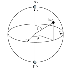
Figure 2.1: Bloch vector $(r_{x},r_{y},r_{z})=(\cos\psi\sin\theta,\sin\psi\sin\theta,\cos\theta)$

For $\tau=(\mathbb{I}+\vec{t}\cdot\vec{\sigma})/2$ with $\vec{t}=(t_{x},t_{y},t_{z})$ we then have

$$D(\rho,\tau)=\frac{1}{2}||\rho-\tau||_{1}=\frac{1}{2}\left|\left|\sum_{j\in\{x,y,z\}}(r_{j}-t_{j})\sigma_{j}\right|\right|_{1}=\frac{1}{2}\sqrt{\sum_{j\in\{x,y,z\}}(r_{j}-t_{j})^{2}},$$

where we used the fact that all Pauli matrices anti-commute. Thus, the trace distance between $\rho$ and $\tau$ is exactly half the Euclidean distance of the corresponding Bloch vectors.

Using the trace distance, we can address the problem of distinguishing two quantum states:

Theorem 2.2.2 (Helstrom [Hel67]).

Suppose we are given states $\rho_{0}$ with probability $q$, and $\rho_{1}$ with probability $1-q$. Then the probability to determine whether the state was $\rho_{0}$ and $\rho_{1}$ is at most

$$p=\frac{1}{2}\left[1+||q\rho_{0}-(1-q)\rho_{1}||_{1}\right].$$

The measurement that achieves $p$ is given by $M_{0}$, and $M_{1}=\mathbb{I}-M_{0}$, where $M_{0}$ is the projector onto the positive eigenspace of $q\rho_{0}-(1-q)\rho_{1}$.

For $q=1/2$, this gives us $p=1/2+D(\rho_{0},\rho_{1})/2$. Indeed, it is easy to see why such $M_{0}$ and $M_{1}$ form the optimal measurement. Note that here we are only interested in finding a POVM. To find the optimal POVM we must solve the following optimization problem for variables $M_{0}$ and $M_{1}$:

maximize	$q\mbox{\rm Tr}(M_{0}\rho_{0})+(1-q)\mbox{\rm Tr}(M_{1}\rho_{1})$
subject to	$M_{0},M_{1}\geq 0$,
	$M_{0}+M_{1}=\mathbb{I}$.

We can rewrite our target function as

$$q\mbox{\rm Tr}(M_{0}\rho_{0})+(1-q)\mbox{\rm Tr}(M_{1}\rho_{1}) = q\mbox{\rm Tr}(M_{0}\rho_{0})+(1-q)\mbox{\rm Tr}((\mathbb{I}-M_{0})\rho_{1})$$

$$= \mbox{\rm Tr}(M_{0}(q\rho_{0}-(1-q)\rho_{1}))+1-q$$

$$= \mbox{\rm Tr}\left(M_{0}\left(\sum_{\lambda_{j}\geq 0}\lambda_{j}|u_{j}\rangle\langle u_{j}|\right)\right)$$

$$+\mbox{\rm Tr}\left(M_{0}\left(\sum_{\lambda_{j}<0}\lambda_{j}|u_{j}\rangle\langle u_{j}|\right)\right)+1-q,$$

where $q\rho_{0}-(1-q)\rho_{1}=\sum_{j}\lambda_{j}|u_{j}\rangle\langle u_{j}|$. Hence, to maximize the above expression, we need to choose $M_{0}=\sum_{\lambda_{j}\geq 0}|u_{j}\rangle\langle u_{j}|$.

Unfortunately, computing the optimal measurement to distinguish more than two states is generally not so easy. Yuen, Kennedy and Lax [YKL75] first showed that this problem can be solved using semidefinite programming, a technique we describe in Appendix A. This technique has since been refined to address other variants such as unambiguous state discrimination where we can output “don’t know”, but are never allowed to make a mistake [Eld03]. Evidently, we can express the optimization problem for any state discrimination problem as

maximize	$\sum_{x}P_{X}(x)\mbox{\rm Tr}(M_{x}\rho_{x})$
subject to	$\forall x\in\mathcal{X},M_{x}\geq 0$,
	$\sum_{x\in\mathcal{X}}M_{x}=\mathbb{I}$.

In Chapter 3, we will use the above formulation. We also show how to address a variant of this problem, where we receive additional classical information after performing the measurement.

Closely related to the trace distance is the notion of fidelity.

Definition 2.2.3.

The fidelity of states $\rho$ and $\sigma$ is given by

$$F(\rho,\sigma)=\mbox{\rm Tr}\sqrt{\rho^{1/2}\sigma\rho^{1/2}}.$$

Note that if $\rho=|\Psi\rangle\langle\Psi|$ is a pure state, this becomes

$$F(|\Psi\rangle,\sigma)=\sqrt{\langle\Psi|\sigma|\Psi\rangle}.$$

The fidelity is closely related to the trace distance. In particular, we have that for any states $\rho$ and $\sigma$

$$1-F(\rho,\sigma)\leq D(\rho,\sigma)\leq\sqrt{1-F(\rho,\sigma)^{2}}.$$

A proof can be found in [NC00, Section 9.2.3]. If $\rho=|\Psi\rangle\langle\Psi|$ is a pure state, the lower bound can be improved to

$$1-F(|\Psi\rangle,\sigma)^{2}\leq D(|\Psi\rangle,\sigma).$$

Many other distance measures of quantum states are known, which may be a more convenient choice for particular problems. We refer to [Fuc95, Hay06] for an overview.

Classical vs. Quantum
Suppose again we are given a classical ensemble of states $\rho$ and $\sigma$. That is, both operators commute and hence have a common eigenbasis $\{|u_{1}\rangle,\ldots,|u_{d}\rangle\}$. We can thus write $\rho=\sum_{j}\lambda_{j}|u_{j}\rangle\langle u_{j}|$ and $\sigma=\sum_{j}\gamma_{j}|u_{j}\rangle\langle u_{j}|$, which allows us to write the trace distance of $\rho$ and $\sigma$ as

$$D(\rho,\sigma)=\frac{||\sum_{j}(\lambda_{j}-\gamma_{j})|u_{j}\rangle\langle u_{j}|||_{1}}{2}=\frac{1}{2}\sum_{j}|\lambda_{j}-\gamma_{j}|=D(\lambda_{j},\gamma_{j}),$$

where $D(\lambda_{j},\gamma_{j})$ is the classical variational distance between the distributions $\{\lambda_{j}\}$ and $\{\gamma_{j}\}$. Again, we see that there is nothing quantum in this setting. We can view $\rho$ and $\sigma$ as two different probability distributions over the set $\{|u_{j}\rangle\}$. Similarly, it is easy to see that

$$F(\rho,\sigma)=\mbox{\rm Tr}\sqrt{\sum_{j}\lambda_{j}\gamma_{j}|u_{j}\rangle\langle u_{j}|}=\sum_{j}\sqrt{\lambda_{j}\gamma_{j}}=F(\lambda_{j},\gamma_{j}),$$

where $F(\lambda_{j},\gamma_{j})$ is the classical fidelity of the distributions $\{\lambda_{j}\}$ and $\{\gamma_{j}\}$.

2.3 Information measures

2.3.1 Classical

We also need the following ways of measuring information. Let $X$ be a random variable distributed over a finite set $\mathcal{X}$ according to probability distribution $P_{X}$. The Shannon entropy of $X$ is then given by

$$H(X)=-\sum_{x\in\mathcal{X}}P_{X}(x)\log P_{X}(x).$$

Intuitively, the Shannon entropy measures how much information we gain on average by learning $X$. A complementary view point is that $H(X)$ quantifies the amount of uncertainty we have about $X$ before the fact. We will also use $H(P_{X})$, if our discussion emphasizes a certain distribution $P_{X}$. If $|\mathcal{X}|=2$, we also use the term binary entropy and use the shorthand

$$h(p)=-p\log p-(1-p)\log(1-p).$$

Let $Y$ be a second random variable distributed over a finite set $\mathcal{Y}$ according to distribution $P_{Y}$. The joint entropy of $X$ and $Y$ can now be expressed as

$$H(X,Y)=-\sum_{x\in\mathcal{X},y\in\mathcal{Y}}P_{XY}(x,y)\log P_{XY}(x,y),$$

where $P_{XY}$ is the joint distribution over $\mathcal{X}\times\mathcal{Y}$. Furthermore, we can quantify the uncertainty about $X$ given $Y$ by means of the conditional entropy

$$H(X|Y)=H(X,Y)-H(Y).$$

To quantify the amount of information $X$ and $Y$ may have in common we use the mutual information

$$\mathcal{I}(X,Y)=H(X)+H(Y)-H(X,Y)=H(X)-H(X|Y).$$

Intuitively the mutual information captures the amount of information we gain about $X$ by learning $Y$. The Shannon entropy has many interesting properties, summarized, for example, in [NC00, Theorem 11.3], but we do not require them here. In Chapter 5, we only need the classical mutual information of a bipartite quantum state $\rho^{AB}$, which is the maximum classical mutual information that can be obtained by local measurements $M^{A}\otimes M^{B}$ on the state $\rho^{AB}$ [THLD02]:

$$\mathcal{I}_{c}(\rho^{AB})=\max_{M^{A}\otimes M^{B}}\mathcal{I}(A,B),$$ (2.2)

where $A$ and $B$ are the random variables corresponding to Alice’s and Bob’s measurement outcomes respectively.

In a cryptographic setting, the Shannon entropy is not always a desirable measure as it merely captures our uncertainty about $X$ on average. Often, the Rényi entropy allows us to make stronger statements The Rényi entropy [Rén60] of order $\alpha$ is defined as

$$H_{\alpha}(X)=\frac{1}{1-\alpha}\log\left[\left(\sum_{x\in\mathcal{X}}P_{X}(x)^{\alpha}\right)^{\frac{1}{\alpha-1}}\right].$$

Indeed, the Shannon entropy forms a special case of the Rényi entropy by taking the limit $\alpha\rightarrow 1$, i.e., $H_{1}(\cdot)=H(\cdot)$, where we omit the subscript. Of particular importance is the min-entropy, for $\alpha\rightarrow\infty$:

$$H_{\infty}(X)=-\log\left(\max_{x\in\mathcal{X}}P_{X}(x)\right),$$

and the collision entropy

$$H_{2}(X)=-\log\sum_{x\in\mathcal{X}}P_{X}(x)^{2}.$$

We have

$$\log|\mathcal{X}|\geq H(X)\geq H_{2}(X)\geq H_{\infty}(X).$$

Intuitively, the min-entropy is determined by the highest peak in the distribution and most closely captures the notion of “guessing” $x$. Consider the following example: Let $\mathcal{X}=\{0,1\}^{n}$ and let $x_{0}=0,\ldots,0$ be the all 0 string. Suppose that $P_{X}(x_{0})=1/2+1/(2^{n+1})$ and $P_{X}(x)=1/(2^{n+1})$ for $x\neq x_{0}$, i.e., with probability $1/2$ we choose $x_{0}$ and with probability $1/2$ we choose one string uniformly at random. Then $H(X)\approx n/2$, whereas $H_{\infty}(X)=1$! If $x$ would correspond to an encryption key used to encrypt an $n$ bit message, we would certainly not talk about security if we can guess the key with probability $1/2$! Yet, the Shannon entropy is quite high. We refer to [Cac97] for an in-depth discussion of security measures in classical cryptography.

2.3.2 Quantum

Similar to the Shannon entropy, the von Neumann entropy of a quantum states $\rho$ is given by

$$S(\rho)=-\mbox{\rm Tr}(\rho\log\rho).$$

Taking the eigendecomposition of $\rho=\sum_{x}\lambda_{x}|x\rangle\langle x|$ we can also write

$$S(\rho)=-\sum_{x}\lambda_{x}\log\lambda_{x},$$

which corresponds to the Shannon entropy arising from measuring $\rho$ in the basis given by $\{|x\rangle\langle x|\}$. We refer to [NC00, Section 11.3] for the properties of the von Neumann entropy.

Here, we will only be concerned with the accessible information [Per93, Eq. (9.75)] of an ensemble $\mathcal{E}=\{p_{x},\rho_{x}\}$ which we encounter again in Chapter 5.

$$\mathcal{I}_{acc}(\mathcal{E})=\max_{M}\left(-\sum_{x}p_{x}\log p_{x}+\right.\left.\sum_{j}\sum_{x}p_{x}\alpha_{j}\mbox{\rm Tr}(M_{j}\rho_{x})\log\frac{p_{x}\mbox{\rm Tr}(M_{j}\rho_{x})}{\mbox{\rm Tr}(M_{j}\rho)}\right),$$

where $\rho=\sum_{x}p_{x}\rho_{x}$ and the maximization is taken over all POVMs $M=\{M_{j}\}$. It has been shown that we can take all POVM elements to be of rank 1 [Dav78]. However, maximizing this quantity still remains a hard task [Per93]. Some upper and lower bounds are known [Fuc95], but sadly none of them are generally very strong. The most well-known upper bound is given by the Holevo quantity, which is given by

$$\chi(\rho)=S(\rho)-\sum_{x}p_{x}S(\rho_{x}).$$

Holevo’s theorem [NC00] states that

$$\mathcal{I}_{acc}(\mathcal{E})\leq\chi(\rho).$$ (2.3)

Classical vs. Quantum
Equality in Eq. (2.3) is achieved if all states $\rho_{x}$ have a common eigenbasis (i.e., all $\rho_{x}$ commute). Hence, for classical ensembles we do not have a gap between these two quantities. The fact that quantumly we can obtain such a gap leads to a peculiar effect known as locking classical information in quantum states in Chapter 5. However, even if the states $\rho_{x}$ do not commute, we can still extract the “classical information” of the ensemble: Suppose for all $\rho_{x}\in\mathcal{H}$ from our ensemble there exists a decomposition $\mathcal{H}=\bigoplus_{j}\mathcal{H}_{j}$ such that for all $x$, $\rho_{x}=\sum_{j}\Pi_{j}\rho_{x}\Pi_{j}$, where $\Pi_{j}$ is a projector onto $\mathcal{H}_{j}$. That is, there exists a way to simultaneously block-diagonalize all states. Note that for any measurement maximizing the accessible information above, we can find an equivalent measurement with measurement operators $\hat{M}=\sum_{j}\Pi_{j}M\Pi_{j}$, since evidently, $\mbox{\rm Tr}(\hat{M}\rho_{x})=\sum_{j}\mbox{\rm Tr}(\Pi_{j}M\Pi_{j}\rho_{x})=\mbox{\rm Tr}(M\rho_{x})$. Intuitively, this means that we can always first determine which block we are in “for free”, followed by our original measurement constrained to this block. Note that $[\Pi_{j},\rho_{x}]=0$ for all $\Pi_{j}$ and $\rho_{x}$. Hence, looking back at Section 2.1.3 this is not so surprising: the measurement leaves our states invariant. In general, such commutation relations lead to interesting structural consequences which we examine in more detail in Appendix B and also exploit in Chapter 3. Finally, it will be useful in Chapter 10 that the accessible information is additive [Hol73, DLT02]: For $m$ independent draws of an ensemble $\mathcal{E}$ of separable states (see Chapter 6), i.e., we choose $m$ states from $m$ identical ensembles independently, we have $\mathcal{I}_{acc}(\mathcal{E}^{\otimes m})=m\mathcal{I}_{acc}(\mathcal{E})$.

2.4 Mutually unbiased bases

In the following chapters, we will be particularly concerned with measurements in mutually unbiased bases (MUBs). MUBs were initially introduced in the context of state estimation [WF89], but feature in many other problems in quantum information. The following definition closely follows the one given in [BBRV02].

Definition 2.4.1 (MUBs).

Let $\mathcal{B}_{1}=\{|b^{1}_{1}\rangle,\ldots,|b^{1}_{d}\rangle\}$ and $\mathcal{B}_{2}=\{|b^{2}_{1}\rangle,\ldots,|b^{2}_{d}\rangle\}$ be two orthonormal bases in $\mathbb{C}^{d}$. They are said to be mutually unbiased if $|\langle{b^{1}_{k}}|{b^{2}_{l}}\rangle|=1/\sqrt{d}$, for every $k,l\in[d]$. A set $\{\mathcal{B}_{1},\ldots,\mathcal{B}_{m}\}$ of orthonormal bases in $\mathbb{C}^{d}$ is called a set of mutually unbiased bases if each pair of bases is mutually unbiased.

As an example, consider the computational and the Hadamard basis defined above, and note that we can write $|+\rangle=H|0\rangle$ and $|-\rangle=H|1\rangle$. We then have for $x\in\{0,1\}^{n}$ that

$$|\langle x|H^{\otimes n}|x\rangle|^{2}=\frac{1}{2^{n}}.$$

Hence, the computational and the Hadamard basis are mutually unbiased in dimension $d=2^{n}$.

We use $N(d)$ to denote the maximal number of MUBs in dimension $d$. In any dimension $d$, we have that $\mbox{N}(d)\leq d+1$ [BBRV02]. If $d=p^{k}$ is a prime power, we have that $\mbox{N}(d)=d+1$ and explicit constructions are known [BBRV02, WF89]. If $d=s^{2}$ is a square, $\mbox{N}(d)\geq\mbox{MOLS}(s)$ where $\mbox{MOLS}(s)$ denotes the number of mutually orthogonal $s\times s$ Latin squares [WB05]. In general, we have $\mbox{N}(nm)\geq\min\{\mbox{N}(n),\mbox{N}(m)\}$ for all $n,m\in\mathbb{N}$ [Zau99, KR03]. It is also known that in any dimension, there exists an explicit construction for 3 MUBs [Gra04]. Unfortunately, not much else is known. For example, it is still an open problem whether there exists a set of $7$ MUBs in dimension $d=6$. We say that a unitary $U_{t}$ transforms the computational basis into the $t$-th MUB $\mathcal{B}_{t}=\{|b^{t}_{1}\rangle,\ldots,|b^{t}_{d}\rangle\}$ if for all $k\in[d]$ we have $|b^{t}_{k}\rangle=U_{t}|k\rangle$. In the next two chapters, we will be particularly concerned with two specific constructions of mutually unbiased bases. There exists a third construction based on Galois rings [KR04], which we do not consider here.

2.4.1 Latin squares

First, we consider MUBs based on mutually orthogonal Latin squares [WB05]. Informally, an $s\times s$ Latin square over the symbol set $[s]$ is an arrangement of elements of $[s]$ into an $s\times s$ square such that in each row and each column every element occurs exactly once. Let $L_{ij}$ denote the entry in a Latin square in row $i$ and column $j$. Two Latin squares $L$ and $L^{\prime}$ are called mutually orthogonal if and only if $\{(L_{i,j},L^{\prime}_{i,j})|i,j\in[s]\}=\{(u,v)|u,v\in[s]\}$. Intuitively, this means that if we place one square on top of the other, and look at all pairs generated by the overlaying elements, all possible pairs occur. An example is given in Figures 2.3 and 2.3 below. From any $s\times s$ Latin square we can obtain a basis for $\mathbb{C}^{s}\otimes\mathbb{C}^{s}$. First, we construct $s$ of the basis vectors from the entries of the Latin square itself. Let

$$|v_{1,\ell}\rangle=\frac{1}{\sqrt{s}}\sum_{i,j\in[s]}E^{L}_{i,j}(\ell)|i,j\rangle,$$

where $E^{L}$ is a predicate such that $E^{L}_{i,j}(\ell)=1$ if and only if $L_{i,j}=\ell$. Note that for each $\ell$ we have exactly $s$ pairs $i,j$ such that $E_{i,j}(\ell)=1$, because each element of $[s]$ occurs exactly $s$ times in the Latin square. Secondly, from each such vector we obtain $s-1$ additional vectors by adding successive rows of an $s\times s$ complex Hadamard matrix $H=(h_{ij})$ as coefficients to obtain the remaining $|v_{t,j}\rangle$ for $t\in[s]$, where $h_{ij}=\omega^{ij}$ with $i,j\in\{0,\ldots,s-1\}$ and $\omega=e^{2\pi i/s}$. Two additional MUBs can then be obtained in the same way from the two non-Latin squares where each element occurs for an entire row or column respectively. From each mutually orthogonal Latin square and these two extra squares which also satisfy the above orthogonality condition, we obtain one basis. This construction therefore gives $\mbox{MOLS}(s)+2$ many MUBs. It is known that if $s=p^{k}$ is a prime power itself, we obtain $p^{k}+1\approx\sqrt{d}$ MUBs from this construction. Note, however, that there do exist many more MUBs in prime power dimensions, namely $d+1$. If $s$ is not a prime power, it is merely known that $\mbox{MOLS}(s)\geq s^{1/14.8}$ [WB05].

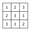
Figure 2.2: Latin Square (LS)

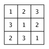
Figure 2.3: Mutually Orthogonal LS

As an example, consider the $3\times 3$ Latin square depicted in Figure 2.3 and the $3\times 3$ complex Hadamard matrix

$$H=\left(\begin{array}[]{ccc}1&1&1\\ 1&\omega&\omega^{2}\\ 1&\omega^{2}&\omega\end{array}\right),$$

where $\omega=e^{2\pi i/3}$. First, we obtain vectors

$$|v_{1,1}\rangle = \frac{1}{\sqrt{3}}(|1,1\rangle+|2,3\rangle+|3,2\rangle)$$

$$|v_{1,2}\rangle = \frac{1}{\sqrt{3}}(|1,2\rangle+|2,1\rangle+|3,3\rangle)$$

$$|v_{1,3}\rangle = \frac{1}{\sqrt{3}}(|1,3\rangle+|2,2\rangle+|3,1\rangle).$$

With the help of $H$ we obtain 3 additional vectors from the ones above. From the vector $|v_{1,1}\rangle$, for example, we obtain

$$|v_{1,1}\rangle = \frac{1}{\sqrt{3}}(|1,1\rangle+|2,3\rangle+|3,2\rangle)$$

$$|v_{2,1}\rangle = \frac{1}{\sqrt{3}}(|1,1\rangle+\omega|2,3\rangle+\omega^{2}|3,2\rangle)$$

$$|v_{3,1}\rangle = \frac{1}{\sqrt{3}}(|1,1\rangle+\omega^{2}|2,3\rangle+\omega|3,2\rangle).$$

This gives us basis $\mathcal{B}=\{|v_{t,\ell}\rangle|t,\ell\in[s]\}$ for $s=3$. The construction of another basis follows in exactly the same way from a mutually orthogonal Latin square. The fact that two such squares $L$ and $L^{\prime}$ are mutually orthogonal ensures that the resulting bases will be mutually unbiased. Indeed, suppose we are given another such basis, $\mathcal{B^{\prime}}=\{|u_{t,\ell}\rangle|t,\ell\in[s]\}$ belonging to $L^{\prime}$. We then have for any $\ell,\ell^{\prime}\in[s]$ that $|\langle{u_{1,\ell^{\prime}}}|{v_{1,\ell}}\rangle|^{2}=|(1/s)\sum_{i,j\in[s]}E^{L^{\prime}}_{i,j}(\ell^{\prime})E^{L}_{i,j}(\ell)|^{2}=1/s^{2}$, as there exists exactly only one pair $\ell,\ell^{\prime}\in[s]$ such that $E^{L^{\prime}}_{i,j}(\ell^{\prime})E^{L}_{i,j}(\ell)=1$. Clearly, the same argument holds for the additional vectors derived from the complex Hadamard matrix.

2.4.2 Generalized Pauli matrices

The second construction we consider is based on the generalized Pauli matrices $X_{d}$ and $Z_{d}$ [BBRV02], defined by their actions on the computational basis $C=\{|0\rangle,\ldots,|d-1\rangle\}$ as follows:

$$X_{d}|k\rangle = |k+1\mod d\rangle$$

$$Z_{d}|k\rangle = \omega^{k}|k\rangle,~{}\forall|k\rangle\in C,$$

where $\omega=e^{2\pi i/d}$. We say that $\left(X_{d}\right)^{a_{1}}\left(Z_{d}\right)^{b_{1}}\otimes\cdots\otimes\left(X_{d}\right)^{a_{N}}\left(Z_{d}\right)^{b_{N}}$ for $a_{k},b_{k}\in\{0,\ldots,d-1\}$ and $k\in[N]$ is a string of Pauli matrices.

If $d$ is a prime, it is known that the $d+1$ MUBs constructed first by Wootters and Fields [WF89] can also be obtained as the eigenvectors of the matrices $Z_{d},X_{d},X_{d}Z_{d},X_{d}Z_{d}^{2},\ldots,X_{d}Z_{d}^{d-1}$ [BBRV02]. If $d=p^{k}$ is a prime power, consider all $d^{2}-1$ possible strings of Pauli matrices excluding the identity and group them into sets $C_{1},\ldots,C_{d+1}$ such that $|C_{i}|=d-1$ and $C_{i}\cap C_{j}=\{\mathbb{I}\}$ for $i\neq j$ and all elements of $C_{i}$ commute. Let $B_{i}$ be the common eigenbasis of all elements of $C_{i}$. Then $B_{1},\ldots,B_{d+1}$ are MUBs [BBRV02]. A similar result for $d=2^{k}$ has also been shown in [LBZ02]. A special case of this construction are the three mutually unbiased bases in dimension $d=2^{k}$ given by the unitaries $\mathbb{I}^{\otimes k}$,$H^{\otimes k}$ and $K^{\otimes k}$ (as defined on page 2.1.3) applied to the computational basis.

2.5 Conclusion

We summarized the most important elements of quantum theory that we need here. We refer to [Per93, NC00, Hay06] for more information about each topic. In Chapters 4 and 6 we investigate the two most striking aspects of quantum theory in detail: uncertainty relations and entanglement. But first, let’s examine the case of state discrimination with additional post-measurement information.

Chapter 3 State discrimination
with post-measurement information

In this chapter, we investigate an extension of the traditional state discrimination problem we encountered in Chapter 2.2: what if we are given some additional information after the measurement? Imagine that you are given a string $x$ encoded in an unknown basis chosen from a known set of bases. You may perform any measurement, but you can only store at most $q$ qubits of quantum information afterwards. Later on, you are told which basis was used. How well can you compute a function $f$ of $x$, given the initial measurement outcome, the $q$ qubits and the additional basis information?

3.1 Introduction

This question is of central importance for protocols in the bounded quantum storage model [DFSS05], which we encountered in Chapter 1. The security of such protocols rests on the realistic assumption that a dishonest player cannot store more than $q$ qubits for long periods of time. In this model, even bit commitment and oblivious transfer can be implemented securely which is otherwise known to be impossible as we saw in Chapter 1. We formalize this general setting as a state discrimination problem: Here, we are given additional information about the state after the measurement or, more generally, after a quantum memory bound is applied. We prove general bounds on the success probability for any balanced function. We also show that storing just a single qubit allows you to compute any Boolean function perfectly when two bases are used. However, we also construct three bases for which you need to keep all qubits.

In general, we consider the following problem: Take an ensemble of quantum states, ${\cal E}=\{p_{yb},\rho_{yb}\}$, with double indices $yb\in{\cal Y}\times{\cal B}$, and an integer $q\geq 0$. Suppose Alice sends Bob the state $\rho_{yb}$, where she alone knows indices $y$ and $b$. Bob can perform any measurement on his system, but afterwards store at most $q$ qubits, and an unlimited amount of classical information. Afterwards, Alice tells him $b$. Bob’s goal is now to approximate $y$ as accurately as possible, which means that he has to make a guess $\hat{Y}$ that maximizes the success probability $P_{\rm succ}=\sum_{yb}p_{yb}\Pr[\hat{Y}=y|\text{state }\rho_{yb}].$ For $|{\cal B}|=1$, i.e., no post-measurement information is available, $q$ is irrelevant and Bob’s task is to discriminate among states $\rho_{y}$. This is the well-known state discrimination problem, which we encountered in Chapter 2.2, a problem studied since the early days of quantum information science.

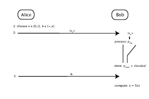
Figure 3.1: Using post-measurement information.

A particular case that isolates the aspect of the timing between measurements and side-information is one where for each fixed $b$, the states $\rho_{yb}$ are mutually orthogonal: if Bob knew $b$, he could actually compute $y$ perfectly. A special case of this problem is depicted in Figure 3.1. Here, Alice picks a string $x\in_{R}\{0,1\}^{n}$, and a basis $b\in\{+,\times\}$. She then encodes the string in the chosen basis and sends the resulting state to Bob. Bob’s goal is now to determine $y=f(x)$ for a fixed function $f$. The states in this particular problem are thus of the form $\rho_{yb}=\sum_{x\in f^{-1}(y)}P_{X|B=b}(x)U_{b}|x\rangle\langle x|U_{b}^{\dagger}$, for a function $f:{\cal X}\rightarrow{\cal Y}$, and a set of mutually unbiased bases (MUBs) ${\cal B}$, given by the unitaries $U_{0}=\mathbb{I},U_{1},\ldots,U_{|{\cal B}|-1}$ on a Hilbert space with basis $\{|x\rangle:x\in{\cal X}\}$, where the string $x$ and a basis $b$ are drawn from the distribution $P_{X,B}$. We mostly focus on this special case.

This problem also has an interpretation in terms of communication complexity. Suppose Alice is given $b$, and Bob is given the state $\rho_{yb}$. If classical communication is free, what is the minimum number of qubits Bob needs to send to Alice such that Alice learns $y$? Note that Bob needs to send exactly $q$ qubits if and only if there exists a strategy for Bob to compute $y$ in our task, while storing only $q$ qubits.

3.1.1 Outline

In the following, we will close in on our problem in several stages. First, we briefly recall the case of state discrimination without any post-measurement information in Section 3.3. This enables us to draw comparisons later.

Second, in Section 3.4 we assume that Bob does receive post-measurement information, but has no quantum memory at all, i.e. $q=0$. His goal then is to compute $f(x)$ given the classical outcome obtained by measuring $U_{b}|x\rangle$ and the later announcement of $b$. Clearly, a trivial strategy for Bob is to simply guess the basis, measure to obtain some string $\hat{x}$ and take $\hat{y}=f(\hat{x})$ as his answer. We thus want to find a better strategy. In particular, we will see that for any number of MUBs, any number of function outcomes, and any balanced $f$, Bob has a systematic advantage over guessing the basis, independent of $|{\cal X}|$. Furthermore, we show that for any Boolean $f$, Bob can succeed with probability at least $P_{succ}\geq 1/2+1/(2\sqrt{2})$ even if he cannot store any qubits at all. The latter result is relevant to the question of whether deterministic privacy amplification is possible in the protocols of [DFSS05]. Here, Alice uses two MUBs, and secretly chooses a function from a set of predetermined functions. She later tells Bob which function he should evaluate, together with the basis information $b$. Is it possible to use a fixed Boolean function instead? Our result shows that this is not possible.

It is interesting to consider when post-measurement information is useful for Bob, and how large his advantage is compared to the case where he does not receive any post-measurement information. To this end, we show how to phrase our problem as a semidefinite program (SDP), in the case where Bob has no quantum memory. In Section 3.4.2, we examine in detail the specific functions XOR and AND, for which we prove optimal bounds on Bob’s success probability. In particular, the XOR on uniformly distributed strings of length $n$ with two or three MUBs provides an extreme example of the usefulness of post-measurement information: We show that for the XOR function with $n$ odd, $P_{\rm succ}=1/2+1/(2\sqrt{2})$. This is the same as Bob can achieve without the extra basis information. For even $n$, $P_{\rm succ}=1$ with the additional basis information. Here, $P_{\rm succ}$ jumps from $3/4$ (without) to certainty (with basis information). The advantage that Bob gains can thus be maximal: without the post-measurement information, he can do no better than guessing the basis. However, with it, he can compute $y=f(x)$ perfectly. For even $n$, this was also observed in [DFSS05]. However, our analysis for odd $n$ shows that the strategy for even $n$ does not work for any linear function as claimed in [DFSS05]. It remains an interesting question to find general conditions on the ensemble of states that determine how useful post-measurement information can be. We return to this question in Chapter 6.4.

Finally, we address the case where Bob does have quantum memory available. The question we are then interested in is: How large does this memory have to be so that Bob can compute $y$ perfectly? In Section 3.5.1, we derive general conditions that determine when $q$ qubits are sufficient. Our conditions impose a restriction on the rank of Bob’s measurement operators and require that all such operators commute with the projector onto the support of $\rho_{yb}$, for all $y$ and $b$. In particular, we give a general algebraic framework that allows us to determine $q$ for any number of bases, functions and outcomes, in combination with an algorithm given in [KI02]. In Sections 3.5.2 and 3.5.3, we then consider two specific examples: First, we show that for any Boolean $f$ and any two bases, storing just a single qubit is sufficient for Bob to compute $f(x)$ perfectly. The latter result again has implications to protocols in the bounded quantum storage model: for all existing protocols, deterministic privacy amplification is indeed hopeless. It turns out that part of this specific example also follows from known results derived for non-local games as we will discuss below. Surprisingly, things change dramatically when we are allowed to use three bases: We show how to construct three bases, such that for any balanced $f$ Bob needs to keep all qubits in order to compute $f(x)$ perfectly!

3.1.2 Related work

In Chapter 2.2, we already examined the traditional setting of state discrimination without post-measurement information. Some of the tools we need below have found use in this setting as well. Many convex optimization problems can be solved using semidefinite programming. We refer to Appendix A for a introduction. Eldar [Eld03] and Eldar, Megretski and Verghese [EMV03] used semidefinite programming to solve state discrimination problems, which is one of the techniques we also use here. The square-root measurement [HW94] (also called pretty good measurement) is an easily constructed measurement to distinguish quantum states, however, it is only optimal for very specific sets of states [EF01, EMV04]. Mochon constructed specific pure state discrimination problems for which the square-root measurement is optimal [Moc07a]. We use a variant of the square-root measurement as well. Furthermore, our problem is related to the task of state filtering [BHH03, BHH05, BH05] and state classification [WY06]. Here, Bob’s goal is to determine whether a given state is either one specific state or one of several other possible states, or, more generally, which subset of states a given state belongs to. Our scenario differs, because we deal with mixed states and Bob is allowed to use post-measurement information. Much more is known about pure state discrimination problems and the case of unambiguous state discrimination where we are not allowed to make an error. Since we concentrate on mixed states, we refer to [BHH04] for an excellent survey on the extended field of state discrimination.

Regarding state discrimination with post-measurement information, special instances of the general problem have occurred in the literature under the heading “mean king’s problem” [AE01, KR05], where the stress was on the usefulness of entanglement. Furthermore, it should be noted that prepare-and-measure quantum key distribution schemes of the BB84 type also lead to special cases of this problem: When considering optimal individual attacks, the eavesdropper is faced with the task of extracting maximal information about the raw key bits, encoded in an unknown basis, that she learns later during basis reconciliation.

Our result that one qubit of storage suffices for any Boolean function $f$ demonstrates that storing quantum information can give an adversary a great advantage over storing merely classical information. It has also been shown in the context of randomness extraction with respect to a quantum adversary that storing quantum information can sometimes convey much more power to the adversary [GKK⁺06].

3.2 Preliminaries

3.2.1 Notation and tools

We need the following notions. The Bell basis is given by the vectors $|\Phi^{\pm}\rangle=(|00\rangle\pm|11\rangle)/\sqrt{2}$ and $|\Psi^{\pm}\rangle=(|01\rangle\pm|10\rangle)/\sqrt{2}$. Furthermore, let $f^{-1}(y)=\{x\in\mathcal{X}|f(x)=y\}$. We say that a function $f$ is balanced if and only if any element in the image of $f$ is generated by equally many elements in the pre-image of $f$, i.e. there exists a $k\in\mathbb{N}$ such that $\forall y\in\mathcal{Y}:|f^{-1}(y)|=k$.

3.2.2 Definitions

We now give a more formal description of our problem. Let $\mathcal{Y}$ and $\mathcal{B}$ be finite sets and let $P_{YB}=\{p_{yb}\}$ be a probability distribution over $\mathcal{Y}\times\mathcal{B}$. Consider an ensemble of quantum states $\mathcal{E}=\{p_{yb},\rho_{yb}\}$. We assume that $\mathcal{Y}$, $\mathcal{B}$, $\mathcal{E}$ and $P_{YB}$ are known to both Alice and Bob. Suppose now that Alice chooses $yb\in\mathcal{Y}\times\mathcal{B}$ according to probability distribution $P_{YB}$, and sends $\rho_{yb}$ to Bob. We can then define the tasks:

Definition 3.2.1.

State discRimination ($\text{\emph{STAR}}(\mathcal{E})$) is the following task for Bob. Given $\rho_{yb}$, determine $y$. He can perform any measurement on $\rho_{yb}$ immediately upon receipt.

Definition 3.2.2.

State discRimination with Post-measurement Information ($\text{\emph{PI}}_{q}\text{\emph{-STAR}}(\mathcal{E})$) is the following task for Bob. Given $\rho_{yb}$, determine $y$, where Bob can use the following sources of information in succession:

1. First, he can perform any measurement on $\rho_{yb}$ immediately upon reception. Afterwards, he can store at most $q$ qubits of quantum information about $\rho_{yb}$, and an unlimited amount of classical information.

2. After Bob’s measurement, Alice announces $b$.

3. Then, he may perform any measurement on the remaining $q$ qubits depending on $b$ and the measurement outcome obtained in step 1.

We also say that Bob succeeds at $\text{\emph{STAR}}(\mathcal{E})$ or $\text{\emph{PI}}_{q}\text{\text{-STAR}}(\mathcal{E})$ with probability $p$ if and only if $p$ is the average success probability $p=\sum_{yb}p_{yb}\Pr[\hat{Y}=y|\text{state }\rho_{yb}]$, where $\Pr[\hat{Y}=y|\text{state }\rho_{yb}]$ is the probability that Bob correctly determines $y$ given $\rho_{yb}$ in the case of STAR, and in addition using information sources 1, 2 and 3 in the case of PI-STAR.

Here, we are interested in the following special case: Consider a function $f:\mathcal{X}\rightarrow\mathcal{Y}$ between finite sets, and a set of mutually unbiased bases $\mathcal{B}$ as defined in Chapter 2, generated by a set of unitaries $U_{0},U_{1},\ldots,U_{|\mathcal{B}|-1}$ acting on a Hilbert space with basis {$|x\rangle\mid x\in\mathcal{X}$}. Take $|\Phi_{b}^{x}\rangle=U_{b}|x\rangle$. Let $P_{X}$ and $P_{B}$ be probability distributions over $\mathcal{X}$ and $\mathcal{B}$ respectively. We assume that $f$, $\mathcal{X}$, $\mathcal{Y}$, $\mathcal{B}$, $P_{X}$, $P_{B}$, and the set of unitaries $\{U_{b}|b\in\mathcal{B}\}$ are known to both Alice and Bob. Suppose now that Alice chooses $x\in\mathcal{X}$ and $b\in\mathcal{B}$ independently according to probability distributions $P_{X}$ and $P_{B}$ respectively, and sends $|\Phi_{b}^{x}\rangle$ to Bob. Bob’s goal is now to compute $y=f(x)$. We thus obtain an instance of our problem with states $\rho_{yb}=\sum_{x\in f^{-1}(y)}P_{X}(x)|\Phi_{b}^{x}\rangle\langle\Phi_{b}^{x}|$. We write $\text{STAR}(f)$ and $\text{PI}_{q}\text{-STAR}(f)$ to denote both problems in this special case. We concentrate on the case of mutually unbiased bases, as this case is most relevant to our initial goal of analyzing protocols for quantum cryptography in the bounded storage model [DFSS05].

Here, we make use of the basis set $\mathcal{B}=\{+,\times,\odot\}$, where $\mathcal{B}_{+}=\{|0\rangle,|1\rangle\}$ is the computational basis, $\mathcal{B}_{\times}=\{\frac{1}{\sqrt{2}}(|0\rangle+|1\rangle),\frac{1}{\sqrt{2}}(|0\rangle-|1\rangle)\}$ is the Hadamard basis, and $\mathcal{B}_{\odot}=\{\frac{1}{\sqrt{2}}(|0\rangle+i|1\rangle),\frac{1}{\sqrt{2}}(|0\rangle-i|1\rangle)\}$ is what we call the K-basis. The unitaries that give rise to these bases are $U_{+}=\mathbb{I}$, $U_{\times}=H$ and $U_{\odot}=K$ with $K=(\mathbb{I}+i\sigma_{x})/\sqrt{2}$ respectively. Recall from Chapter 2 that the Hadamard matrix is given by $H=\frac{1}{\sqrt{2}}(\sigma_{x}+\sigma_{z})$, and that $\sigma_{x}$, $\sigma_{z}$ and $\sigma_{y}$ are the well-known Pauli matrices. We generally assume that Bob has no a priori knowledge about the outcome of the function and about the value of $b$. This means that $b$ is chosen uniformly at random from $\mathcal{B}$, and, in the case of balanced functions, that Alice chooses $x$ uniformly at random from $\mathcal{X}$. More generally, the distribution is uniform on all $f^{-1}(y)$ and such that each value $y\in{\cal Y}$ is equally likely.

3.2.3 A trivial bound: guessing the basis

Note that a simple strategy for Bob is to guess the basis, and then measure. This approach leads to a lower bound on the success probability for both STAR and PI-STAR. In short:

Lemma 3.2.3.

Let $P_{X}(x)=\frac{1}{2^{n}}$ for all $x\in\{0,1\}^{n}$. Let $\mathcal{B}$ denote the set of bases. Then for any balanced function $f:\mathcal{X}\rightarrow\mathcal{Y}$ Bob succeeds at $\text{\emph{STAR}}(f)$ and $\text{\emph{PI}}_{0}\text{\emph{-STAR}}(f)$ with probability at least

$$p_{\text{guess}}=\frac{1}{|\mathcal{B}|}+\left(1-\frac{1}{|\mathcal{B}|}\right)\frac{1}{|\mathcal{Y}|}.$$

Our goal is to beat this bound. We show that for PI-STAR, Bob can indeed do much better.

3.3 No post-measurement information

We first consider the standard case of state discrimination. Here, Alice does not supply Bob with any additional post-measurement information. Instead, Bob’s goal is to compute $y=f(x)$ immediately. This analysis enables us to gain interesting insights into the usefulness of post-measurement information later.

3.3.1 Two simple examples

We now examine two simple one-qubit examples of a state discrimination problem, which we make use of later on. Here, Bob’s goal is to learn the value of a bit which has been encoded in two or three mutually unbiased bases while he does not know which basis has been used.

Lemma 3.3.1.

Let $x\in\{0,1\}$, $P_{X}(x)=\frac{1}{2}$ and $f(x)=x$. Let $\mathcal{B}=\{+,\times\}$ with $U_{+}=\mathbb{I}$ and $U_{\times}=H$. Then Bob succeeds at $\text{\emph{STAR}}(f)$ with probability at most

$$p=\frac{1}{2}+\frac{1}{2\sqrt{2}}.$$

There exists a strategy for Bob that achieves $p$.

Proof 3.3.2.

The probability of success follows from Theorem 2.2.2 with $\rho_{0}=\frac{1}{2}(|0\rangle\langle 0|+H|0\rangle\langle 0|H)$, $\rho_{1}=\frac{1}{2}(|1\rangle\langle 1|+H|1\rangle\langle 1|H)$ and $q=1/2$.

Lemma 3.3.3.

Let $x\in\{0,1\}$, $P_{X}(x)=\frac{1}{2}$ and $f(x)=x$. Let $\mathcal{B}=\{+,\times,\odot\}$ with $U_{+}=\mathbb{I}$, $U_{\times}=H$ and $U_{\odot}=K$. Then Bob succeeds at $\text{\emph{STAR}}(f)$ with probability at most

$$p=\frac{1}{2}+\frac{1}{2\sqrt{3}}.$$

There exists a strategy for Bob that achieves $p$.

Proof 3.3.4.

The proof is identical to that of Lemma 3.3.1 using $\rho_{0}=\frac{1}{3}(|0\rangle\langle 0|+H|0\rangle\langle 0|H+K|0\rangle\langle 0|K^{\dagger})$, $\rho_{1}=\frac{1}{3}(|1\rangle\langle 1|+H|1\rangle\langle 1|H+K|1\rangle\langle 1|K^{\dagger})$, and $q=1/2$.

3.3.2 An upper bound for all Boolean functions

We now show that for any Boolean function $f$ and any number of mutually unbiased bases, the probability that Bob succeeds at $\text{STAR}(f)$ is very limited.

Theorem 3.3.5.

Let $|\mathcal{Y}|=2$ and let $f$ be a balanced function. Let $\mathcal{B}$ be a set of mutually unbiased bases. Then Bob succeeds at $\text{\emph{STAR}}(f)$ with probability at most

$$p=\frac{1}{2}+\frac{1}{2\sqrt{|\mathcal{B}|}}.$$

In particular, for $|\mathcal{B}|=2$ we obtain $(1+1/\sqrt{2})/2\approx 0.853$; for $|\mathcal{B}|=3$, we obtain $(1+1/\sqrt{3})/2\approx 0.789$.

Proof 3.3.6.

The probability of success is given by Theorem 2.2.2 where for $y\in\{0,1\}$

$$\rho_{y}=\frac{1}{2^{n-1}|\mathcal{B}|}\sum_{b=0}^{|\mathcal{B}|-1}P_{yb},$$

with $P_{yb}=\sum_{x\in f^{-1}(y)}U_{b}|x\rangle\langle x|U_{b}^{\dagger}$. Using the Cauchy-Schwarz inequality we can show that

$$\|\rho_{0}-\rho_{1}\|_{1}^{2}=[\mbox{\rm Tr}(|\rho_{0}-\rho_{1}|\mathbb{I})]^{2}\leq\mbox{\rm Tr}[(\rho_{0}-\rho_{1})^{2}]\mbox{\rm Tr}[\mathbb{I}^{2}]=2^{n}\mbox{\rm Tr}[(\rho_{0}-\rho_{1})^{2}],$$ (3.1)

or

$$\|\rho_{0}-\rho_{1}\|_{1}\leq\sqrt{2^{n}\mbox{\rm Tr}[(\rho_{0}-\rho_{1})^{2}]}.$$

A simple calculation shows that

$$\mbox{\rm Tr}[(\rho_{0}-\rho_{1})^{2}]=\frac{4}{2^{n}|\mathcal{B}|}.$$

The theorem follows from the previous equation, together with Theorem 2.2.2 and Eq. (3.1).

3.3.3 AND function

One of the simplest functions to consider is the AND function. Recall, that we always assume that Bob has no a priori knowledge about the outcome of the function. In the case of the AND, this means that we are considering a very specific prior: with probability $1/2$ Alice will choose the only string $x$ for which $\text{AND}(x)=1$. Without any post-measurement information, Bob can already compute the AND quite well.

Theorem 3.3.7.

Let $P_{X}(x)=1/(2(2^{n}-1))$ for all $x\in\{0,1\}^{n}\setminus\{1\ldots 1\}$ and $P_{X}(1\ldots 1)=\frac{1}{2}$. Let $\mathcal{B}=\{+,\times\}$ with $U_{+}=\mathbb{I}^{\otimes n}$, $U_{\times}=H^{\otimes n}$ and $P_{B}(+)=P_{B}(\times)=1/2$. Then Bob succeeds at $\text{\emph{STAR}}(\text{\emph{AND}})$ with probability at most

$$p=\left\{\begin{array}[]{ll}\frac{1}{2}+\frac{1}{2\sqrt{2}}&\textrm{ if }n=1,\\ 1-\frac{1}{2(2^{n}-1)}&\textrm{ if }n\geq 2.\end{array}\right.$$ (3.2)

There exists a strategy for Bob that achieves $p$.

Proof 3.3.8.

Let $|c_{1}\rangle=|1\rangle^{\otimes n}$ and $|h_{1}\rangle=[H|1\rangle]^{\otimes n}$. Eq. (3.2) is obtained by substituting

$$\rho_{0} = \frac{1}{2}\left[\frac{\mathbb{I}-|c_{1}\rangle\langle c_{1}|}{2^{n}-1}+\frac{\mathbb{I}-|h_{1}\rangle\langle h_{1}|}{2^{n}-1}\right],$$

$$\rho_{1} = \frac{|c_{1}\rangle\langle c_{1}|+|h_{1}\rangle\langle h_{1}|}{2},$$

and $q=1/2$ in Theorem 2.2.2.

In Theorem 3.4.4, we show an optimal bound for the case that Bob does indeed receive the extra information. By comparing the previous equation with Eq. (3.4) later on, we can see that for $n=1$ announcing the basis does not help. However, for $n>1$ we will observe an improvement of $[2(2^{n}+2^{n/2}-2)]^{-1}$.

3.3.4 XOR function

The XOR function provides an example of a Boolean function where we observe both the largest advantage as well as the smallest advantage in receiving post-measurement information: For strings of even length we show that without the extra information Bob can never do better than guessing the basis. For strings of odd length, however, he can do quite a bit better. Interestingly, it turns out that in this case the post-measurement information is completely useless to him. We first investigate how well Bob does at $\text{STAR}(\text{XOR})$ for two bases:

Theorem 3.3.9.

Let $P_{X}(x)=\frac{1}{2^{n}}$ for all $x\in\{0,1\}^{n}$. Let $\mathcal{B}=\{+,\times\}$ with $U_{+}=\mathbb{I}^{\otimes n}$, $U_{\times}=H^{\otimes n}$ and $P_{B}(+)=P_{B}(\times)=1/2$. Then Bob succeeds at $\text{\emph{STAR}}(\text{\emph{XOR}})$ with probability at most

$$p=\begin{cases}\frac{3}{4}&\text{ if }$n$\text{ is even},\\ \frac{1}{2}\left(1+\frac{1}{\sqrt{2}}\right)&\text{ if }$n$\text{ is odd}.\end{cases}$$

There exists a strategy for Bob that achieves $p$.

Proof 3.3.10.

Our proof works by induction on $n$. The case of $n=1$ was addressed in Lemma 3.3.1. Now, consider $n=2$: Let $\sigma^{(2)}_{0}=\frac{1}{2}(\rho^{(2)}_{0+}+\rho^{(2)}_{0\times})$ and $\sigma^{(2)}_{1}=\frac{1}{2}(\rho^{(2)}_{1+}+\rho^{(2)}_{1\times})$, where $\rho^{(2)}_{0+}$ and $\rho^{(2)}_{1+}$ are defined as $\rho^{(n)}_{yb}=\frac{1}{2^{n-1}}\sum_{x\in\{0,1\}^{n},x\in\text{XOR}^{-1}(y)}U_{b}|x\rangle\langle x|U_{b}^{\dagger}$ with $y\in\{0,1\}$ and $b\in\mathcal{B}=\{+,\times\}$. A straightforward calculation shows that $\|\sigma^{(2)}_{0}-\sigma^{(2)}_{1}\|_{1}=1$.

We now show that the trace distance does not change when we go from strings of length $n$ to strings of length $n+2$: Note that we can write

$$\begin{aligned} \rho_{0+}^{(n+2)}&=\frac{1}{2}(\rho^{(n)}_{0+}\otimes\rho^{(2)}_{0+}+\rho^{(n)}_{1+}\otimes\rho^{(2)}_{1+})\\ \rho_{0\times}^{(n+2)}&=\frac{1}{2}(\rho^{(n)}_{0\times}\otimes\rho^{(2)}_{0\times}+\rho^{(n)}_{1\times}\otimes\rho^{(2)}_{1\times})\\ \rho_{1+}^{(n+2)}&=\frac{1}{2}(\rho^{(n)}_{0+}\otimes\rho^{(2)}_{1+}+\rho^{(n)}_{1+}\otimes\rho^{(2)}_{0+})\\ \rho_{1\times}^{(n+2)}&=\frac{1}{2}(\rho^{(n)}_{0\times}\otimes\rho^{(1)}_{1\times}+\rho^{(n)}_{1\times}\otimes\rho^{(2)}_{0\times}).\end{aligned}$$ (3.3)

Let $\sigma^{(n)}_{0}=\frac{1}{2}(\rho^{(n)}_{0+}+\rho^{(n)}_{0\times})$ and $\sigma^{(n)}_{1}=\frac{1}{2}(\rho^{(n)}_{1+}+\rho^{(n)}_{1\times})$. A small calculation shows that

$$\begin{split}\sigma^{(n+2)}_{0}-\sigma^{(n+2)}_{1}&=\frac{1}{8}\bigl{[}(\rho^{(n)}_{0+}+\rho^{(n)}_{0\times}-\rho^{(n)}_{1+}-\rho^{(n)}_{1\times})\otimes|\Phi^{+}\rangle\langle\Phi^{+}|\bigr{.}\\ &\phantom{===}-(\rho^{(n)}_{0+}+\rho^{(n)}_{0\times}-\rho^{(n)}_{1+}-\rho^{(n)}_{1\times})\otimes|\Psi^{-}\rangle\langle\Psi^{-}|\\ &\phantom{===}+(\rho^{(n)}_{0+}+\rho^{(n)}_{1\times}-\rho^{(n)}_{1+}-\rho^{(n)}_{0\times})\otimes|\Phi^{-}\rangle\langle\Phi^{-}|\\ &\phantom{===}-\bigl{.}(\rho^{(n)}_{0+}+\rho^{(n)}_{1\times}-\rho^{(n)}_{1+}-\rho^{(n)}_{0\times})\otimes|\Psi^{+}\rangle\langle\Psi^{+}|\bigr{]}\end{split}$$

We then get that

$$\|\sigma^{(n+2)}_{0}-\sigma^{(n+2)}_{1}\|_{1}=\frac{1}{2}\left(\|\sigma^{(n)}_{0}-\sigma^{(n)}_{1}\|_{1}+\|\tilde{\sigma}^{(n)}_{0}-\tilde{\sigma}^{(n)}_{1}\|_{1}\right),$$

where $\tilde{\sigma}^{(n)}_{0}=\frac{1}{2}(\rho^{(n)}_{0+}+\rho^{(n)}_{1\times})$ and $\tilde{\sigma}^{(n)}_{1}=\frac{1}{2}(\rho^{(n)}_{1+}+\rho^{(n)}_{0\times})$. Consider the unitary $U=\sigma_{x}^{\otimes n}$ if $n$ is odd, and $U=\sigma_{x}^{\otimes n-1}\otimes\mathbb{I}$ if $n$ is even. It is easy to verify that $\sigma^{(n)}_{0}=U\tilde{\sigma}^{(n)}_{0}U^{\dagger}$ and $\sigma^{(n)}_{1}=U\tilde{\sigma}^{(n)}_{1}U^{\dagger}$. We thus have that $\|\sigma^{(n)}_{0}-\sigma^{(n)}_{1}\|_{1}=\|\tilde{\sigma}^{(n)}_{0}-\tilde{\sigma}^{(n)}_{1}\|_{1}$ and therefore

$$\|\sigma^{(n+2)}_{0}-\sigma^{(n+2)}_{1}\|_{1}=\|\sigma^{(n)}_{0}-\sigma^{(n)}_{1}\|_{1}.$$

It then follows from Helstrom’s Theorem 2.2.2 that the maximum probability to distinguish $\sigma^{(n+2)}_{0}$ from $\sigma^{(n+2)}_{1}$ and thus compute the XOR of the $n+2$ bits is given by

$$\frac{1}{2}+\frac{\|\sigma^{(n)}_{0}-\sigma^{(n)}_{1}\|_{1}}{4},$$

which gives the claimed result.

A similar argument is possible, if we use three mutually unbiased bases. Intuitively, one might expect Bob’s chance of success to drop as we had more bases. Interestingly, however, we obtain the same bound of 3/4 if $n$ is even.

Theorem 3.3.11.

Let $P_{X}(x)=\frac{1}{2^{n}}$ for all $x\in\{0,1\}^{n}$. Let $\mathcal{B}=\{+,\times,\odot\}$ with $U_{+}=\mathbb{I}^{\otimes n}$, $U_{\times}=H^{\otimes n}$, and $U_{\odot}=K^{\otimes n}$ with $P_{B}(+)=P_{B}(\times)=P_{B}(\odot)=1/3$. Then Bob succeeds at $\text{\emph{STAR}}(\text{\emph{XOR}})$ with probability at most

$$p=\begin{cases}\frac{3}{4}&\text{ if }$n$\text{ is even},\\ \frac{1}{2}\left(1+\frac{1}{\sqrt{3}}\right)&\text{ if }$n$\text{ is odd}.\end{cases}$$

There exists a strategy for Bob that achieves $p$.

Proof 3.3.12.

Our proof is very similar to the case of only 2 mutually unbiased bases. The case of $n=1$ follows from Lemma 3.3.3. This time, we have for $n=2$: $\sigma^{(2)}_{0}=\frac{1}{3}(\rho^{(2)}_{0+}+\rho^{(2)}_{0\times}+\rho^{(2)}_{0\odot})$ and $\sigma^{(2)}_{1}=\frac{1}{3}(\rho^{(2)}_{1+}+\rho^{(2)}_{1\times}+\rho^{(2)}_{1\odot})$. We have $\|\sigma^{(2)}_{0}-\sigma^{(2)}_{1}\|_{1}=1$.

We again show that the trace distance does not change when we go from strings of length $n$ to strings of length $n+2$. We use the definitions from Eq. (3.3) and let

$$\rho_{0\odot}^{(n+2)} = \frac{1}{2}(\rho^{(n)}_{0\odot}\otimes\rho^{(2)}_{0\odot}+\rho^{(n)}_{1\odot}\otimes\rho^{(2)}_{1\odot}),$$

$$\rho_{1\odot}^{(n+2)} = \frac{1}{2}(\rho^{(n)}_{0\odot}\otimes\rho^{(2)}_{1\odot}+\rho^{(n)}_{1\odot}\otimes\rho^{(2)}_{0\odot}).$$

We can compute

$$\begin{split}\sigma^{(n+2)}_{0}-\sigma^{(n+2)}_{1}&=\frac{1}{4}\bigl{[}(\bar{\sigma}^{(n)}_{1}-\bar{\sigma}^{(n)}_{0})\otimes|\Phi^{+}\rangle\langle\Phi^{+}|\bigr{.}\\ &\phantom{===}-(\hat{\sigma}^{(n)}_{1}-\hat{\sigma}^{(n)}_{0})\otimes|\Psi^{-}\rangle\langle\Psi^{-}|\\ &\phantom{===}+(\tilde{\sigma}^{(n)}_{1}-\tilde{\sigma}^{(n)}_{0})\otimes|\Phi^{-}\rangle\langle\Phi^{-}|\\ &\phantom{===}-\bigl{.}(\sigma^{(n)}_{1}-\sigma^{(n)}_{0})\otimes|\Psi^{+}\rangle\langle\Psi^{+}|\bigr{]},\end{split}$$

where $\bar{\sigma}^{(n)}_{1}=(\rho^{(n)}_{0+}+\rho^{(n)}_{0\times}+\rho^{(n)}_{1\odot})/3$, $\bar{\sigma}^{(n)}_{0}=(\rho^{(n)}_{1+}+\rho^{(n)}_{1\times}+\rho^{(n)}_{0\odot})/3$, $\hat{\sigma}^{(n)}_{1}=(\rho^{(n)}_{0+}+\rho^{(n)}_{1\times}+\rho^{(n)}_{0\odot})/3$, $\hat{\sigma}^{(n)}_{0}=(\rho^{(n)}_{1+}+\rho^{(n)}_{0\times}+\rho^{(n)}_{1\odot})/3$, $\tilde{\sigma}^{(n)}_{0}=(\rho^{(n)}_{1+}+\rho^{(n)}_{0\times}+\rho^{(n)}_{0\odot})/3$, and $\tilde{\sigma}^{(n)}_{0}=(\rho^{(n)}_{0+}+\rho^{(n)}_{1\times}+\rho^{(n)}_{1\odot})/3$. Consider the unitaries $\bar{U}=\sigma_{y}^{\otimes n}$, $\hat{U}=\sigma_{x}^{\otimes n}$, and $\tilde{U}=\sigma_{z}^{\otimes n}$ if $n$ is odd, and $\bar{U}=\sigma_{y}^{\otimes n-1}\otimes\mathbb{I}$, $\hat{U}=\sigma_{x}^{\otimes n-1}\otimes\mathbb{I}$, and $\tilde{U}=\sigma_{z}^{\otimes n-1}\otimes\mathbb{I}$ if $n$ is even. It is easily verified that $\sigma^{(n)}_{0}=\bar{U}\bar{\sigma}^{(n)}_{0}\bar{U}^{\dagger}$, $\sigma^{(n)}_{1}=\bar{U}\bar{\sigma}^{(n)}_{1}\bar{U}^{\dagger}$, $\sigma^{(n)}_{0}=\hat{U}\hat{\sigma}^{(n)}_{0}\hat{U}^{\dagger}$, $\sigma^{(n)}_{1}=\hat{U}\hat{\sigma}^{(n)}_{1}\hat{U}^{\dagger}$, $\sigma^{(n)}_{0}=\tilde{U}\tilde{\sigma}^{(n)}_{0}\tilde{U}^{\dagger}$, and $\sigma^{(n)}_{1}=\tilde{U}\tilde{\sigma}^{(n)}_{1}\tilde{U}^{\dagger}$. We then get that

$$\|\sigma^{(n+2)}_{0}-\sigma^{(n+2)}_{1}\|_{1}=\|\sigma^{(n)}_{0}-\sigma^{(n)}_{1}\|_{1},$$

from which the claim follows.

Surprisingly, if Bob does have some a priori knowledge about the outcome of the XOR the problem becomes much harder for Bob. By expressing the states in the Bell basis and using Helstrom’s result, it is easy to see that if Alice chooses $x\in\{0,1\}^{2}$ such that with probability $q$, $\text{XOR}(x)=0$, and with probability $(1-q)$, $\text{XOR}(x)=1$, Bob’s probability of learning $\text{XOR}(x)$ correctly is minimized for $q=1/3$. In that case, Bob succeeds with probability at most $2/3$, which can be achieved by the trivial strategy of ignoring the state he received and always outputting 1. This is an explicit example where making a measurement does not help in state discrimination. It has previously been noted by Hunter [Hun03] that such cases can exist in mixed-state discrimination.

3.4 Using post-measurement information

We are now ready to advance to the core of our problem. We first consider the case where Bob does receive post-measurement information, but still has no quantum memory at his disposal. Consider an instance of $\text{PI}_{0}\text{-STAR}$ with a function $f:\mathcal{X}\rightarrow\mathcal{Y}$ and $m=|\mathcal{B}|$ bases, and some priors $P_{X}$ and $P_{B}$ on the sets $\mathcal{X}$ and $\mathcal{B}$. If Bob cannot store any quantum information, all his nontrivial actions are contained in the first measurement, which must equip him with possible outputs $o_{i}\in\mathcal{Y}$ for each basis $i=1,\ldots,m$. In other words, his most general strategy is a POVM with $|\mathcal{Y}|^{m}$ outcomes, each labeled by the strings $o_{1},\ldots,o_{m}$ for $o_{i}\in\mathcal{Y}$ and $m=|\mathcal{B}|$. Once Alice has announced $b$, Bob outputs $\hat{Y}=o_{b}$. Here we first prove a general lower bound on the usefulness of post-measurement information that beats the guessing bound. Then, we analyze in detail the AND and the XOR function on $n$ bits.

3.4.1 A lower bound for balanced functions

We first give a lower bound on Bob’s success probability for any balanced function and any number of mutually unbiased bases, by constructing an explicit measurement that achieves it. Without loss of generality, we assume in this section that $\mathcal{B}=\{0,\ldots,m-1\}$, as otherwise we could consider a lexicographic ordering of $\mathcal{B}$.

Theorem 3.4.1.

Let $f:\mathcal{X}\rightarrow\mathcal{Y}$ be a balanced function, and let $P_{X}$ and $P_{B}$ be the uniform distributions over $\mathcal{X}$ and $\mathcal{B}$ respectively. Let the set of unitaries $\{U_{b}|b\in\mathcal{B}\}$ give rise to $|\mathcal{B}|$ mutually unbiased bases, and choose an encoding such that $\forall x,x^{\prime}\in\mathcal{X}:\langle{x}|{x^{\prime}}\rangle=\delta_{xx^{\prime}}$. Then Bob succeeds at $\text{\emph{PI}}_{0}\text{\emph{-STAR}}(f)$ with probability at least

$$p=p_{\text{guess}}+\begin{cases}\frac{|\mathcal{Y}|-1}{|\mathcal{Y}|(|\mathcal{Y}|+3)}&\text{ if }m=2,\\ \frac{4(|\mathcal{Y}|^{2}-1)}{3|\mathcal{Y}|(2+|\mathcal{Y}|(|\mathcal{Y}|+6))}&\text{ if }m=3,\\ -\frac{2}{2|\mathcal{Y}|}+\frac{2(|\mathcal{Y}|+m-1)}{|\mathcal{Y}|^{2}+3|\mathcal{Y}|(m-1)+m^{2}-3m+2}&\text{ if }m\geq 4.\end{cases}$$

where $p_{\text{guess}}$ is the probability that Bob can achieve by guessing the basis as given in Lemma 3.2.3. In particular, we always have $p>p_{\text{guess}}$.

Proof 3.4.2.

Our proof works by constructing a square-root type measurement that achieves the lower bound. As explained above, Bob’s strategy for learning $f(x)$ is to perform a measurement with $|\mathcal{Y}|^{m}$ possible outcomes, labeled by the strings $o_{1},\ldots,o_{m}$ for $o_{i}\in\mathcal{Y}$ and $m=|\mathcal{B}|$. Once Alice has announced $b$, Bob outputs $f(x)=o_{b}$.

Take the projector $P_{yb}=\sum_{x\in f^{-1}(y)}|\Phi^{x}_{b}\rangle\langle\Phi^{x}_{b}|$ and $\rho_{yb}=\frac{1}{k}P_{yb}$, where $k=|f^{-1}(y)|=|\mathcal{X}|/|\mathcal{Y}|$. Let $M_{o_{1},\ldots,o_{m}}$ denote the measurement operator corresponding to outcome $o_{1},\ldots,o_{m}$. Note that outcome $o_{1},\ldots,o_{m}$ is the correct outcome for input state $\rho_{yb}$ if and only if $o_{b}=y$. We can then write Bob’s probability of success as

$$\frac{1}{m|\mathcal{Y}|}\sum_{o_{1},\ldots,o_{m}\in\mathcal{Y}}\mbox{\rm Tr}\left(M_{o_{1},\ldots,o_{m}}\left(\sum_{b\in\mathcal{B}}\rho_{o_{b}b}\right)\right).$$

We make use of the following measurement:

$$M_{o_{1},\ldots,o_{m}}=S^{-\frac{1}{2}}\left(\sum_{b\in\mathcal{B}}P_{o_{b}b}\right)^{3}S^{-\frac{1}{2}},\text{ with }S=\sum_{o_{1},\ldots,o_{m}\in\mathcal{Y}}\left(\sum_{b\in\mathcal{B}}P_{o_{b}b}\right)^{3}.$$

Clearly, we have $\sum_{o_{1},\ldots,o_{m}\in\mathcal{Y}}M_{o_{1},\ldots,o_{m}}=\mathbb{I}$ and $\forall o_{1},\ldots,o_{m}\in\mathcal{Y}:M_{o_{1},\ldots,o_{m}}\geq 0$ by construction and thus we indeed have a valid measurement. We first show that $S=c_{m}\mathbb{I}$:

$$\begin{split}S&=\sum_{o_{1},\ldots,o_{m}\in\mathcal{Y}}\left(\sum_{b\in\mathcal{B}}P_{o_{b}b}\right)^{3}\\ =&\sum_{o_{1},\ldots,o_{m}\in\mathcal{Y}}\sum_{b,b^{\prime},b^{\prime\prime}\in\mathcal{B}}P_{o_{b}b}P_{o_{b^{\prime}}b^{\prime}}P_{o_{b^{\prime\prime}}b^{\prime\prime}}\\ =&\sum_{o_{1},\ldots,o_{m}\in\mathcal{Y}}\left(\sum_{b}P_{o_{b}b}+2\sum_{bb^{\prime},b\neq b^{\prime}}P_{o_{b}b}P_{o_{b^{\prime}}b^{\prime}}\right.\\ &\phantom{========}\left.+\sum_{bb^{\prime},b\neq b^{\prime}}P_{o_{b}b}P_{o_{b^{\prime}}b^{\prime}}P_{o_{b}b}+\sum_{bb^{\prime}b^{\prime\prime},b\neq b^{\prime},b\neq b^{\prime\prime},b^{\prime}\neq b^{\prime\prime}}P_{o_{b}b}P_{o_{b^{\prime}}b^{\prime}}P_{o_{b^{\prime\prime}}b^{\prime\prime}}\right)\\ =&\bigl{[}m|\mathcal{Y}|^{m-1}+2m(m-1)|\mathcal{Y}|^{m-2}+m(m-1)|\mathcal{Y}|^{m-2}+m(m-1)(m-2)|\mathcal{Y}|^{m-3}\bar{\delta}_{2m}\bigr{]}\mathbb{I},\end{split}$$

where $\bar{\delta}_{2m}=1-\delta_{2m}$ and we have used the definition that for any $b$, $P_{o_{b}b}$ is a projector and $\sum_{x\in\mathcal{X}}|\Phi_{b}^{x}\rangle\langle\Phi_{b}^{x}|=\mathbb{I}$ which gives $\sum_{o_{i}\in\mathcal{Y}}P_{o_{i}b_{i}}=\sum_{o_{i}\in\mathcal{Y}}\sum_{x\in f^{-1}(y)}|\Phi_{b}^{x}\rangle\langle\Phi_{b}^{x}|=\mathbb{I}$. We can then write Bob’s probability of success using this particular measurement as

$$\frac{1}{c_{m}km|\mathcal{Y}|}\sum_{o_{1},\ldots,o_{m}\in\mathcal{Y}}\mbox{\rm Tr}\left(\left(\sum_{b\in\mathcal{B}}P_{o_{b}b}\right)^{4}\right).$$

It remains to evaluate this expression. Using the circularity of the trace, we obtain

$$\begin{split}&\sum_{o_{1},\ldots,o_{m}\in\mathcal{Y}}\mbox{\rm Tr}\left(\left(\sum_{b\in\mathcal{B}}P_{o_{b}b}\right)^{4}\right)\\ &=\sum_{o_{1},\ldots,o_{m}\in\mathcal{Y}}\mbox{\rm Tr}\left(\sum_{b}P_{o_{b}b}+6\sum_{bb^{\prime},b\neq b^{\prime}}P_{o_{b}b}P_{o_{b^{\prime}}b^{\prime}}\right.\\ &\phantom{=}+4\sum_{bb^{\prime}b^{\prime\prime},b\neq b^{\prime},b\neq b^{\prime\prime},b^{\prime}\neq b^{\prime\prime}}P_{o_{b}b}P_{o_{b^{\prime}}b^{\prime}}P_{o_{b^{\prime\prime}}b^{\prime\prime}}+2\sum_{bb^{\prime}b^{\prime\prime},b\neq b^{\prime},b\neq b^{\prime\prime},b^{\prime}\neq b^{\prime\prime}}P_{o_{b}b}P_{o_{b^{\prime}}b^{\prime}}P_{o_{b}b}P_{o_{b^{\prime\prime}}b^{\prime\prime}}\\ &\phantom{=}+\left.\sum_{bb^{\prime}b^{\prime\prime}\tilde{b},b\neq b^{\prime},b\neq b^{\prime\prime},b\neq\tilde{b},b^{\prime}\neq b^{\prime\prime},b^{\prime}\neq\tilde{b},b^{\prime\prime}\neq\tilde{b}}P_{o_{b}b}P_{o_{b^{\prime}}b^{\prime}}P_{o_{b^{\prime\prime}}b^{\prime\prime}}P_{o_{\tilde{b}}\tilde{b}}+\sum_{bb^{\prime},b\neq b^{\prime}}P_{o_{b}b}P_{o_{b^{\prime}}b^{\prime}}P_{o_{b}b}P_{o_{b^{\prime}}b^{\prime}}\right)\\ &\geq\bigl{[}m|\mathcal{Y}|^{m-1}+6m(m-1)|\mathcal{Y}|^{m-2}+6m(m-1)(m-2)|\mathcal{Y}|^{m-3}\bar{\delta}_{2m}\bigr{.}\\ &\phantom{==}+\bigl{.}m(m-1)(m-2)(m-3)|\mathcal{Y}|^{t(m-4)}\bar{\delta}_{2m}\bar{\delta}_{3m}\bigr{]}\mbox{\rm Tr}(\mathbb{I})+m(m-1)|\mathcal{Y}|^{m-2}k,\end{split}$$

where we have again used the assumption that for any $b$, $P_{o_{b}b}$ is a projector and $\sum_{x\in\mathcal{X}}|\Phi_{b}^{x}\rangle\langle\Phi_{b}^{x}|=\mathbb{I}$ with $\mbox{\rm Tr}(\mathbb{I})=|\mathcal{X}|$. For the last term we have used the following: Note that $\mbox{\rm Tr}(P_{o_{b}b}P_{o_{b^{\prime}}b^{\prime}})=k^{2}/|\mathcal{X}|$, because we assumed mutually unbiased bases. Let $r=\mbox{rank}(P_{o_{b}b}P_{o_{b^{\prime}}b^{\prime}})$. Using Cauchy-Schwarz, we can then bound $\mbox{\rm Tr}((P_{o_{b}b}P_{o_{b^{\prime}}b^{\prime}})^{2})=\sum_{i}^{r}\lambda_{i}(P_{o_{b}b}P_{o_{b^{\prime}}b^{\prime}})^{2}\geq k^{4}/(|\mathcal{X}|^{2}r)\geq k^{3}/|\mathcal{X}|^{2}=k/|\mathcal{Y}|^{2}$, where $\lambda_{i}(A)$ is the $i$-th eigenvalue of a matrix $A$, by noting that $r\leq k$ since $\mbox{rank}(P_{o_{b}b})=\mbox{rank}(P_{o_{b}^{\prime}b^{\prime}})=k$. Putting things together we obtain

$$p\geq\frac{1}{c_{m}m}\left[G_{m}(1)+\left(6+\frac{1}{|\mathcal{Y}|}\right)G_{m}(2)+6G_{m}(3)+G_{m}(4)\right],$$

where $m=|\mathcal{B}|$, $c_{m}=G_{m}(1)+3G_{m}(2)+G_{m}(3)$ and function $G_{m}:\mathbb{N}\rightarrow\mathbb{N}$ defined as $G_{m}(i)=\frac{m!}{(m-i)!}|\mathcal{Y}|^{m-i}\prod_{j=2}^{i-1}\bar{\delta}_{mj}.$ This expression can be simplified to obtain the claimed result.

Note that we have only used the assumption that Alice uses mutually unbiased bases in the very last step to say that $\mbox{\rm Tr}(P_{o_{b}b}P_{o_{b^{\prime}}b^{\prime}})=k^{2}/|\mathcal{X}|$. One could generalize our argument to other cases by evaluating $\mbox{\rm Tr}(P_{o_{b}b}P_{o_{b^{\prime}}b^{\prime}})$ approximately.

In the special case $m=|{\cal Y}|=2$ (i.e. binary function, with two bases) we obtain:

Corollary 3.4.3.

Let $f:\{0,1\}^{n}\rightarrow\{0,1\}$ be a balanced function and let $P_{X}(x)=2^{-n}$ for all $x\in\{0,1\}^{n}$. Let $\mathcal{B}=\{0,1\}$ with $U_{0}=\mathbb{I}^{\otimes n}$, $U_{1}=H^{\otimes n}$ and $P_{B}(0)=P_{B}(1)=1/2$. Then Bob succeeds at $\text{\emph{PI}}_{0}\text{\emph{-STAR}}(f)$ with probability $p\geq 0.85$.

Observe that this almost attains the upper bound of $\approx.853$ of Lemma 3.3.1 in the case of no post-measurement information. In Section 3.5.2 we show that indeed this bound can always be achieved when post-measurement information is available.

It is perhaps interesting to note that our general bound depends only on the number of function values $|\mathcal{Y}|$ and the number of bases $m$. The number of function inputs $|\mathcal{X}|$ itself does not play a direct role.

3.4.2 Optimal bounds for the AND and XOR function

We now show that for some specific functions, the probability of success can even be much larger. We hereby concentrate on the case where Alice uses two or three mutually unbiased bases to encode her input. Our proofs thereby lead to explicit measurements. In the following, we again assume that Bob has no a priori knowledge of the function value. It turns out that the optimal measurement directly lead us to the essential idea underlying our algebraic framework of Section 3.5.1.

AND function

Theorem 3.4.4.

Let $P_{X}(x)=1/(2(2^{n}-1))$ for all $x\in\{0,1\}^{n}\setminus\{1\ldots 1\}$ and $P_{X}(1\ldots 1)=\frac{1}{2}$. Let $\mathcal{B}=\{+,\times\}$ with $U_{+}=\mathbb{I}^{\otimes n}$, $U_{\times}=H^{\otimes n}$ and $P_{B}(+)=P_{B}(\times)=1/2$. Then Bob succeeds at $\text{\emph{PI}}_{0}\text{\emph{-STAR}}(\text{\emph{AND}})$ with probability at most

$$p=\frac{1}{2}\left[2+\frac{1}{2^{n}+2^{n/2}-2}-\frac{1}{2^{n}-1}\right].$$ (3.4)

There exists a strategy for Bob that achieves $p$.

Proof 3.4.5.

To learn the value of $\text{AND}(x)$, Bob uses the same strategy as in Section 3.4.1: he performs a measurement with $4$ possible outcomes, labeled by the strings $o_{+},o_{\times}$ with $o_{+},o_{\times}\in\{0,1\}$. Once Alice has announced her basis choice $b\in\{+,\times\}$, Bob outputs $\text{AND}(x)=o_{b}$. Note that without loss of generality we can assume that Bob’s measurement has only $4$ outcomes, i.e. Bob only stores 2 bits of classical information because he will only condition his answer on the value of $b$ later on.

Following the approach in the last section, we can write Bob’s optimal probability of success as a semidefinite program:

maximize	$\frac{1}{4}\sum_{o_{+},o_{\times}\in\{0,1\}}\mbox{\rm Tr}[b_{o_{+}o_{\times}}M_{o_{+}o_{\times}}]$
subject to	$\forall o_{+},o_{\times}\in\{0,1\}:M_{o_{+}o_{\times}}\geq 0$,
	$\sum_{o_{+},o_{\times}\in\{0,1\}}M_{o_{+}o_{\times}}=\mathbb{I}$,

where

$$b_{00}=\rho_{0+}+\rho_{0\times}, b_{01}=\rho_{0+}+\rho_{1\times},$$

$$b_{10}=\rho_{1+}+\rho_{0\times}, b_{11}=\rho_{1+}+\rho_{1\times},$$

with $\forall y\in\{0,1\},b\in\{+,\times\}:\rho_{yb}=\frac{1}{|AND^{-1}(y)|}\sum_{x\in\text{AND}^{-1}(y)}U_{b}|x\rangle\langle x|U_{B}^{\dagger}$. Consider $\mathcal{H}_{2}$, the $2$-dimensional Hilbert space spanned by $|c_{1}\rangle\stackrel{{\scriptstyle\textrm{\tiny def}}}{{=}}|1\rangle^{\otimes n}$ and $|h_{1}\rangle\stackrel{{\scriptstyle\textrm{\tiny def}}}{{=}}|1_{\times}\rangle^{\otimes n}$. Let $|c_{0}\rangle\in\mathcal{H}_{2}$ and $|h_{0}\rangle\in\mathcal{H}_{2}$ be the state vectors orthogonal to $|c_{1}\rangle$ and $|h_{1}\rangle$ respectively. They can be expressed as:

$$|c_{o}\rangle = \frac{(-1)^{n+1}|c_{1}\rangle+2^{n/2}|h_{1}\rangle}{\sqrt{2^{n}-1}},$$

$$|h_{o}\rangle = \frac{2^{n/2}|c_{1}\rangle+(-1)^{n+1}|h_{1}\rangle}{\sqrt{2^{n}-1}}.$$

Then $\Pi_{\parallel}=|c_{0}\rangle\langle c_{0}|+|c_{1}\rangle\langle c_{1}|=|h_{0}\rangle\langle h_{0}|+|h_{1}\rangle\langle h_{1}|$ is a projector onto $\mathcal{H}_{2}$. Let $\Pi_{\perp}$ be a projector onto the orthogonal complement of $\mathcal{H}_{2}$. Note that the $b_{o_{+}o_{\times}}$ are all composed of two blocks, one supported on $\mathcal{H}_{2}$ and the other on its orthogonal complement. We can thus write

$$\begin{aligned} b_{00}&=\frac{2\Pi_{\perp}}{2^{n}-1}&+&\frac{|c_{0}\rangle\langle c_{0}|+|h_{0}\rangle\langle h_{0}|}{2^{n}-1},\\ b_{01}&=\frac{\Pi_{\perp}}{2^{n}-1}&+&\left[\frac{|c_{0}\rangle\langle c_{0}|}{2^{n}-1}+|h_{1}\rangle\langle h_{1}|\right],\\ b_{10}&=\frac{\Pi_{\perp}}{2^{n}-1}&+&\left[\frac{|h_{0}\rangle\langle h_{0}|}{2^{n}-1}+|c_{1}\rangle\langle c_{1}|\right],\\ b_{11}&=0&+&|c_{1}\rangle\langle c_{1}|+|h_{1}\rangle\langle h_{1}|.\end{aligned}$$ (3.5)

We give an explicit measurement that achieves $p$ and then show that it is optimal. Take

$$M_{00} =\Pi_{\perp}$$

$$M_{o_{+}o_{\times}} =\lambda_{o_{+}o_{\times}}|\psi_{o_{+}o_{\times}}\rangle\langle\psi_{o_{+}o_{\times}}|,$$

with $\lambda_{01}=\lambda_{10}=(1+\eta)^{-1}$ where

$$\eta =\left|\frac{1-2\beta^{2}+(-1)^{n+1}2\beta\sqrt{1-\beta^{2}}\sqrt{2^{n}-1}}{2^{n/2}}\right|,$$

$$|\psi_{01}\rangle =\alpha|c_{0}\rangle+\beta|c_{1}\rangle,$$

$$|\psi_{10}\rangle =\alpha|h_{0}\rangle+\beta|h_{1}\rangle,$$

with $\alpha$ and $\beta$ real and satisfying $\alpha^{2}+\beta^{2}=1$. We also set $M_{11}=\mathbb{I}-M_{00}-M_{01}-M_{10}$. We take

$$\beta=(-1)^{n}\frac{1}{\sqrt{2^{2n}+2^{\frac{3}{2}n+1}-2^{\frac{n}{2}+1}}}.$$

Putting it all together, we thus calculate Bob’s probability of success:

$$p=\frac{1}{2}\left[2+\frac{1}{2^{n}+2^{n/2}-2}-\frac{1}{2^{n}-1}\right].$$

We now show that this is in fact the optimal measurement for Bob. For this we consider the dual of our semidefinite program above:

minimize	$\mbox{\rm Tr}(Q)$
subject to	$\forall o_{+},o_{\times}\in\{0,1\}:Q\geq\displaystyle\frac{b_{o_{+}o_{\times}}}{4}$.

Our goal is now to find a $Q$ such that $p=\mbox{\rm Tr}(Q)$ and $Q$ is dual feasible. We can then conclude from the duality of SDP that $p$ is optimal. Consider

$$Q= \frac{\Pi_{\perp}}{2(2^{n}-1)}+\frac{1}{4}\left(\frac{2-{2^{1+n/2}}+{2^{3n/2}}}{2-3\cdot{2^{n/2}}+{2^{3n/2}}}\right)(|c_{1}\rangle\langle c_{1}|+|h_{1}\rangle\langle h_{1}|)$$

$$-(-1)^{n}\frac{1}{4({2^{1-\frac{n}{2}}}+{2^{n}}-3)}(|c_{1}\rangle\langle h_{1}|+|c_{1}\rangle\langle h_{1}|).$$

Now we only need to show that the $Q$ above satisfies the constraints, i.e. $\forall o_{+},o_{\times}\in\{0,1\}:Q\geq b_{o_{+}o_{\times}}/4$. Let $Q_{\perp}=\Pi_{\perp}Q\Pi_{\perp}$ and $Q_{\parallel}=\Pi_{\parallel}Q\Pi_{\parallel}$. By taking a look at Eq. (3.5) one can easily see that $Q_{\perp}\geq\frac{\Pi_{\perp}b_{o_{+}o_{\times}}\Pi_{\perp}}{4},$ so that it is only left to show that

$$Q_{\parallel}\geq\frac{\Pi_{\parallel}b_{o_{+}o_{\times}}\Pi_{\parallel}}{4},\textrm{ for }o_{+}o_{\times}\in\{0,1\},o_{+}o_{\times}\neq 00.$$

These are $2\times 2$ matrices and this can be done straightforwardly. We thus have $\mbox{\rm Tr}(Q)=p$ and the result follows from the duality of semidefinite programming.

It also follows that if Bob just wants to learn the value of a single bit, he can do no better than what he could achieve without waiting for Alice’s announcement of the basis $b$:

Corollary 3.4.6.

Let $x\in\{0,1\}$, $P_{X}(x)=\frac{1}{2}$ and $f(x)=x$. Let $\mathcal{B}=\{+,\times\}$ with $U_{+}=\mathbb{I}$ and $U_{\times}=H$. Then Bob succeeds at $\text{\emph{PI}}_{0}\text{\emph{-STAR}}(f)$ with probability at most

$$p=\frac{1}{2}+\frac{1}{2\sqrt{2}}.$$

There exists a strategy for Bob that achieves $p$.

The AND function provides an intuitive example of how Bob can compute the value of a function perfectly by storing just a single qubit. Consider the measurement with elements $\{\Pi_{\parallel},\Pi_{\perp}\}$ from the previous section. It is easy to see that the outcome $\perp$ has zero probability if $\text{AND}(x)=1$. Thus, if Bob obtains that outcome he can immediately conclude that $\text{AND}(x)=0$. If Bob obtains outcome $\parallel$ then the post-measurement states live in a $2$-dimensional Hilbert space ($\mathcal{H}_{2}$), and can therefore be stored in a single qubit. Thus, by keeping the remaining state we can calculate the AND perfectly once the basis is announced. Our proof in Section 3.5.2, which shows that in fact all Boolean functions can be computed perfectly if Bob can store only a single qubit, makes use of a very similar effect to the one we observed here explicitly.

XOR function

We now examine the XOR function. This will be useful in order to gain some insight into the usefulness of post-measurement information later. For strings of even length, there exists a simple strategy for Bob even when three mutually unbiased bases are used.

Theorem 3.4.7.

Let $n\in\mathbb{N}$ be even, and let $P_{X}(x)=\frac{1}{2^{n}}$ for all $x\in\{0,1\}^{n}$. Let $\mathcal{B}=\{+,\times,\odot\}$ with $U_{+}=\mathbb{I}^{\otimes n}$, $U_{\times}=H^{\otimes n}$ and $U_{\odot}=K^{\otimes n}$, where $K=(\mathbb{I}+i\sigma_{x})/\sqrt{2}$. Then there is a strategy where Bob succeeds at $\text{\emph{PI}}_{0}\text{\emph{-STAR}}(\text{\emph{XOR}})$ with probability $p=1$.

Proof 3.4.8.

We first construct Bob’s measurement for the first 2 qubits, which allows him to learn $x_{1}\oplus x_{2}$ with probability 1. Note that the 12 possible states that Alice sends can be expressed in the Bell basis as follows:

$$|00\rangle=\frac{1}{\sqrt{2}}(|\Phi^{+}\rangle+|\Phi^{-}\rangle) H^{\otimes 2}|00\rangle=\frac{1}{\sqrt{2}}(|\Phi^{+}\rangle+|\Psi^{+}\rangle)$$

$$|01\rangle=\frac{1}{\sqrt{2}}(|\Psi^{+}\rangle+|\Psi^{-}\rangle) H^{\otimes 2}|01\rangle=\frac{1}{\sqrt{2}}(|\Phi^{-}\rangle+|\Psi^{-}\rangle)$$

$$|10\rangle=\frac{1}{\sqrt{2}}(|\Psi^{+}\rangle-|\Psi^{-}\rangle) H^{\otimes 2}|10\rangle=\frac{1}{\sqrt{2}}(|\Phi^{-}\rangle-|\Psi^{-}\rangle)$$

$$|11\rangle=\frac{1}{\sqrt{2}}(|\Phi^{+}\rangle-|\Phi^{-}\rangle) H^{\otimes 2}|11\rangle=\frac{1}{\sqrt{2}}(|\Phi^{+}\rangle-|\Psi^{+}\rangle)$$

$$K^{\otimes 2}|00\rangle = \frac{1}{\sqrt{2}}(|\Phi^{-}\rangle+i|\Psi^{+}\rangle)$$

$$K^{\otimes 2}|01\rangle = \frac{1}{\sqrt{2}}(i|\Phi^{+}\rangle+|\Psi^{-}\rangle)$$

$$K^{\otimes 2}|10\rangle = \frac{1}{\sqrt{2}}(i|\Phi^{+}\rangle-|\Psi^{-}\rangle)$$

$$K^{\otimes 2}|11\rangle = -\frac{1}{\sqrt{2}}(|\Phi^{-}\rangle-i|\Psi^{+}\rangle).$$

Bob now simply measures in the Bell basis and records his outcome. If Alice now announces that she used the computational basis, Bob concludes that $x_{1}\oplus x_{2}=0$ if the outcome is one of $|\Phi^{\pm}\rangle$ and $x_{1}\oplus x_{2}=1$ otherwise. If Alice announces she used the Hadamard basis, Bob concludes that $x_{1}\oplus x_{2}=0$ if the outcome was one of $\{|\Phi^{+}\rangle,|\Psi^{+}\rangle\}$ and $x_{1}\oplus x_{2}=1$ otherwise. Finally, if Alice announces that she used the $\odot$ basis, Bob concludes that $x_{1}\oplus x_{2}=0$ if the outcome was one of $\{|\Phi^{-}\rangle,|\Psi^{+}\rangle\}$ and $x_{1}\oplus x_{2}=1$ otherwise. Bob can thus learn the XOR of two bits with probability 1. To learn the XOR of the entire string, Bob applies this strategy to each two bits individually and then computes the XOR of all answers.

Analogously to the proof of Theorem 3.4.7, we obtain:

Corollary 3.4.9.

Let $n\in\mathbb{N}$ be even, and let $P_{X}(x)=\frac{1}{2^{n}}$ for all $x\in\{0,1\}^{n}$. Let $\mathcal{B}=\{+,\times\}$ with $U_{+}=\mathbb{I}^{\otimes n}$ and $U_{\times}=H^{\otimes n}$. Then there is a strategy where Bob succeeds at $\text{\emph{PI}}_{0}\text{\emph{-STAR}}(\text{\emph{XOR}})$ with probability $p=1$.

Interestingly, there is no equivalent strategy for Bob if $n$ is odd. In fact, as we show in the next section, in this case the post-measurement information gives no advantage to Bob at all.

Theorem 3.4.10.

Let $n\in\mathbb{N}$ be odd, and let $P_{X}(x)=\frac{1}{2^{n}}$ for all $x\in\{0,1\}^{n}$. Let $\mathcal{B}=\{+,\times\}$ with $U_{+}=\mathbb{I}^{\otimes n}$, $U_{\times}=H^{\otimes n}$ and $P_{B}(+)=P_{B}(\times)=1/2$. Then Bob succeeds at $\text{\emph{PI}}_{0}\text{\emph{-STAR}}(\text{\emph{XOR}})$ with probability at most

$$p=\frac{1}{2}\left(1+\frac{1}{\sqrt{2}}\right).$$

There exists a strategy for Bob that achieves $p$.

Proof 3.4.11.

Similar to the proof of the AND function, we can write Bob’s optimal probability of success as the following semidefinite program in terms of the length of the input string, $n$:

maximize	$\frac{1}{4}\sum_{o_{+},o_{\times}\in\{0,1\}}\mbox{\rm Tr}[b^{(n)}_{o_{+}o_{\times}}M_{o_{+}o_{\times}}]$
subject to	$\forall o_{+},o_{\times}\in\{0,1\}:M_{o_{+}o_{\times}}\geq 0$,
	$\sum_{o_{+},o_{\times}\in\{0,1\}}M_{o_{+}o_{\times}}=\mathbb{I}$,

where

$$b^{(n)}_{o_{+}o_{\times}} =\rho^{(n)}_{o_{+}+}+\rho^{(n)}_{o_{\times}\times},$$

and $\rho^{(n)}_{o_{b}b}=\frac{1}{2^{n-1}}\sum_{x\in\{0,1\}^{n},x\in\text{XOR}^{-1}(o_{b})}U_{b}|x\rangle\langle x|U_{b}^{\dagger}$. The dual can be written as

minimize	$\frac{1}{4}\mbox{\rm Tr}(Q^{(n)})$
subject to	$\forall o_{+},o_{\times}\in\{0,1\}:Q^{(n)}\geq\displaystyle b^{(n)}_{o_{+}o_{\times}}$.

Our proof is now by induction on $n$. For $n=1$, let $Q^{(1)}=2p\mathbb{I}$. It is easy to verify that $\forall o_{+},o_{\times}\in\{0,1\}:Q^{(1)}\geq b^{(1)}_{o_{+}o_{\times}}$ and thus $Q^{(1)}$ is a feasible solution of the dual program.

We now show that for $n+2$, $Q^{(n+2)}=Q^{(n)}\otimes\frac{1}{4}\mathbb{I}$ is a feasible solution to the dual for $n+2$, where $Q^{(n)}$ is a solution for the dual for $n$. Note that the XOR of all bits in the string can be expressed as the XOR of the first $n-2$ bits XORed with the XOR of the last two. Recall Eq. (3.3) and note that we can write

$$\rho^{(2)}_{0+} =\frac{1}{2}(|00\rangle\langle 00|+|11\rangle\langle 11|)=\frac{1}{2}(|\Phi^{+}\rangle\langle\Phi^{+}|+|\Phi^{-}\rangle\langle\Phi^{-}|)$$

$$\rho^{(2)}_{1+} =\frac{1}{2}(|01\rangle\langle 01|+|10\rangle\langle 10|)=\frac{1}{2}(|\Psi^{+}\rangle\langle\Psi^{+}|+|\Psi^{-}\rangle\langle\Psi^{-}|).$$

It is easy to see that $\rho^{(2)}_{0\times}=H\rho^{(2)}_{0+}H=\frac{1}{2}(|\Phi^{+}\rangle\langle\Phi^{+}|+|\Psi^{+}\rangle\langle\Psi^{+}|)$ and $\rho^{(2)}_{1\times}=H\rho^{(2)}_{1+}H=\frac{1}{2}(|\Phi^{-}\rangle\langle\Phi^{-}|+|\Psi^{-}\rangle\langle\Psi^{-}|)$. By substituting from the above equation we then obtain

$$\begin{split}b^{(n+2)}_{00}=\rho^{(n+2)}_{0+}+\rho^{(n+2)}_{0\times}&=\frac{1}{4}\bigl{(}(\rho^{(n)}_{0+}+\rho^{(n)}_{0\times})\otimes|\Phi^{+}\rangle\langle\Phi^{+}|+(\rho^{(n)}_{0+}+\rho^{(n)}_{1\times})\otimes|\Phi^{-}\rangle\langle\Phi^{-}|\bigr{.}\\ &\phantom{==}\bigl{.}(\rho^{(n)}_{1+}+\rho^{(n)}_{0\times})\otimes|\Psi^{+}\rangle\langle\Psi^{+}|+(\rho^{(n)}_{1+}+\rho^{(n)}_{1\times})\otimes|\Psi^{-}\rangle\langle\Psi^{-}|)\bigr{)}\\ &\leq\frac{1}{4}Q^{(n)}\otimes\mathbb{I},\end{split}$$

where we have used the fact that $Q^{(n)}$ is a feasible solution for the dual for $n$ and that $|\Phi^{+}\rangle\langle\Phi^{+}|+|\Phi^{-}\rangle\langle\Phi^{-}|+|\Psi^{+}\rangle\langle\Psi^{+}|+|\Psi^{-}\rangle\langle\Psi^{-}|=\mathbb{I}$. The argument for $b^{(n+2)}_{01}$, $b^{(n+2)}_{10}$ and $b^{(n+2)}_{11}$ is analogous. Thus $Q^{(n+2)}$ satisfies all constraints.

Putting things together, we have for odd $n$ that $\mbox{\rm Tr}(Q^{(n+2)})=\mbox{\rm Tr}(Q^{(n)})=\mbox{\rm Tr}(Q^{(1)})$ and since the dual is a minimization problem we know that

$$p\leq\frac{1}{4}\mbox{\rm Tr}(Q^{(1)})=c$$

as claimed. Clearly, there exists a strategy for Bob that achieves $p=c$. He can compute the XOR of the first $n-1$ bits perfectly, as shown in Theorem 3.4.9. By Corollary 3.4.6 he can learn the value of the remaining $n$-th bit with probability $p=c$.

We obtain a similar bound for three bases:

Theorem 3.4.12.

Let $n\in\mathbb{N}$ be odd, and let $P_{X}(x)=\frac{1}{2^{n}}$ for all $x\in\{0,1\}^{n}$. Let $\mathcal{B}=\{+,\times,\odot\}$ with $U_{+}=\mathbb{I}^{\otimes n}$, $U_{\times}=H^{\otimes n}$ and $U_{\odot}=K^{\otimes n}$, where $K=(\mathbb{I}+i\sigma_{x})/\sqrt{2}$, with $P_{B}(+)=P_{B}(\times)=P_{B}(\odot)=1/3$. Then Bob succeeds at $\text{\emph{PI}}_{0}\text{\emph{-STAR}}(\text{\emph{XOR}})$ with probability at most

$$p=\frac{1}{2}\left(1+\frac{1}{\sqrt{3}}\right).$$

There exists a strategy for Bob that achieves $p$.

Proof 3.4.13.

The proof follows the same lines as Theorem 3.4.10. Bob’s optimal probability of success is:

maximize	$\displaystyle\frac{1}{6}\sum_{o_{+},o_{\times},o_{\odot}\in\{0,1\}}\mbox{\rm Tr}[b^{(n)}_{o_{+}o_{\times}o_{\odot}}M_{o_{+}o_{\times}o_{\odot}}]$
subject to	$\forall o_{+},o_{\times},o_{\odot}\in\{0,1\}\in\{0,1\}:M_{o_{+}o_{\times}o_{\odot}}\geq 0$,
	$\displaystyle\sum_{o_{+},o_{\times},o_{\odot}\in\{0,1\}}M_{o_{+}o_{\times}o_{\odot}}=\mathbb{I}$,

where

$$b^{(n)}_{o_{+}o_{\times}o_{\odot}}=\sum_{b\in\mathcal{B}}\rho_{o_{b}b},$$

and

$$\rho_{o_{b}b}=\frac{1}{2^{n-1}}\sum_{x\in XOR(o_{b})}U_{b}|x\rangle\langle x|U_{b}^{\dagger}.$$

The dual can be written as

minimize	$\frac{1}{6}\mbox{\rm Tr}(Q^{(n)})$
subject to	$\forall o_{+},o_{\times},o_{\odot}\in\{0,1\}:Q^{(n)}\geq\displaystyle b^{(n)}_{o_{+}o_{\times}o_{\odot}}$.

Again, the proof continues by induction on $n$. For $n=1$, let $Q^{(1)}=3p\mathbb{I}$. It is easy to verify that $\forall o_{+},o_{\times},o_{\odot}\in\{0,1\}:Q^{(1)}\geq b^{(1)}_{o_{+}o_{\times}o_{\odot}}$ and thus $Q^{(1)}$ is a feasible solution of the dual program. The rest of the proof is done exactly in the same way as in Theorem 3.4.10 using that

$$\rho^{(2)}_{0\odot} =\frac{1}{2}(|\Phi^{-}\rangle\langle\Phi^{-}|+|\Psi^{+}\rangle\langle\Psi^{+}|)$$

$$\rho^{(2)}_{1\odot} =\frac{1}{2}(|\Psi^{-}\rangle\langle\Psi^{-}|+|\Phi^{+}\rangle\langle\Phi^{+}|).$$

3.5 Using post-measurement information
and quantum memory

3.5.1 An algebraic framework for perfect prediction

So far, we had assumed that Bob is not allowed to store any qubits and can only use the additional post-measurement information to improve his guess. Now, we investigate the case where he has a certain amount of quantum memory at his disposal. In particular, we present a general algebraic approach to determine the minimum dimension $2^{q}$ of quantum memory needed to succeed with probability $1$ at an instance of $\text{PI}_{q}\text{-STAR}(\mathcal{E})$, for any ensemble $\mathcal{E}=\{p_{yb},\rho_{yb}\}$ as long as the individual states for different values of $y$ are mutually orthogonal for a fixed $b$, i.e., $\forall y\neq z\in\mathcal{Y}\>\mbox{\rm Tr}(\rho_{yb},\rho_{zb})=0$. In particular, we are looking for an instrument consisting of a family of completely positive maps $\rho\mapsto A\rho A^{\dagger}$, adding up to a trace preserving map, such that $\mbox{rank}(A)\leq 2^{q}$. This ensures that the post-measurement state “fits” into $q$ qubits, and thus takes care of the memory bound. The fact that after the announcement of $b$ the remaining state $A\rho_{yb}A^{\dagger}$ gives full information about $y$ is expressed by demanding orthogonality of the different post-measurement states:

$$\forall b\in\mathcal{B},\forall y\neq z\in\mathcal{Y}\quad A\rho_{yb}A^{\dagger}A\rho_{zb}A^{\dagger}=0.$$ (3.6)

Note that here we explicitly allow the possibility that, say, $A\rho_{zb}A^{\dagger}=0$: this means that if Bob obtains outcome $A$ and later learns $b$, he can exclude the output value $z$. What Eq. (3.6) also implies is that for all states $|\psi\rangle$ and $|\varphi\rangle$ in the support of $\rho_{yb}$ and $\rho_{zb}$, respectively, one has $A|\psi\rangle\langle\psi|A^{\dagger}A|\varphi\rangle\langle\varphi|A^{\dagger}=0$. Hence, introducing the support projectors $P_{yb}$ of the $\rho_{yb}$, we can reformulate Eq. (3.6) as

$$\forall b\in\mathcal{B},\forall y\neq z\in\mathcal{Y}\quad AP_{yb}A^{\dagger}AP_{zb}A^{\dagger}=0,$$

which can equivalently be expressed as

$$\forall b\in\mathcal{B},\forall y\neq z\in\mathcal{Y}\quad\mbox{\rm Tr}\bigl{(}A^{\dagger}AP_{yb}A^{\dagger}AP_{zb}\bigr{)}=0,$$ (3.7)

by noting that $A^{\dagger}A$ as well as the projectors are positive-semidefinite operators. As expected, we see that only the POVM operators $M=A^{\dagger}A$ of the instrument play a role in this condition. Our conditions can therefore also be written as $MP_{yb}MP_{zb}=0$. From this condition, we now derive the following lemma.

Lemma 3.5.1.

Bob, using a POVM with operators $\{M_{i}\}$, succeeds at $\text{PI}_{q}\text{-STAR}$ with probability $1$, if and only if

1. for all $i$, $\mbox{rank}(M_{i})\leq 2^{q}$,

2. for all $y\in\mathcal{Y}$ and $b\in\mathcal{B}$, $[M,P_{yb}]=0$, where $P_{yb}$ is the projection on the support of $\rho_{yb}$.

Proof 3.5.2.

We first show that these two conditions are necessary. Note that only the commutation condition has to be proved. Let $M$ be a measurement operator from a POVM succeeding with probability $1$. Then, for any $y$, $b$, we have by Eq. (3.7) that

$$\mbox{\rm Tr}\bigl{(}MP_{yb}M(\mathbb{I}-P_{yb})\bigr{)}=0,\text{ hence }\mbox{\rm Tr}\bigl{(}MP_{yb}MP_{yb}\bigr{)}=\mbox{\rm Tr}\bigl{(}MP_{yb}M\bigr{)}.$$

Thus, by the positivity of the trace on positive operators, the cyclicity of the trace, and $P_{yb}^{2}=P_{yb}$ we have that

$$\begin{split}0&\leq\mbox{\rm Tr}\bigl{(}[M,P_{yb}]^{\dagger}[M,P_{yb}]\bigr{)}\\ &=\mbox{\rm Tr}\bigl{(}-(MP_{yb}-P_{yb}M)^{2}\bigr{)}\\ &=\mbox{\rm Tr}\bigl{(}-MP_{yb}MP_{yb}-P_{yb}MP_{yb}M+P_{yb}M^{2}P_{yb}+MP_{yb}^{2}M\bigr{)}=0.\end{split}$$

But that means that the commutator $[M,P_{yb}]$ has to be $0$.

Sufficiency is easy: since the measurement operators commute with the states’ support projectors $P_{yb}$, and these are orthogonal to each other for fixed $b$, the post-measurement states of these projectors, $\propto\sqrt{M}P_{yb}\sqrt{M}$ are also mutually orthogonal for fixed $b$. Thus, if Bob learns $b$, he can perform a measurement to distinguish the different values of $y$ perfectly. The post-measurement states are clearly supported on the support of $M$, which can be stored in $q$ qubits. Since Bob’s strategy succeeds with probability $1$, it succeeds with probability $1$ for any states supported in the range of the $P_{yb}$.

Note that the operators $M$ of the instrument need not commute with the originally given states $\rho_{yb}$. Nevertheless, the measurement preserves the orthogonality of $\rho_{yb}$ and $\rho_{zb}$ with $y\neq z$ for fixed $b$, i.e., $\mbox{\rm Tr}(\rho_{yb}\rho_{zb})=0$. Now that we know that the POVM operators of the instrument have to commute with all the states’ support projectors $P_{yb}$, we can invoke some well-developed algebraic machinery to find the optimal such instrument.

Looking at Appendix B, we see that $M$ has to come from the commutant of the operators $P_{yb}$. These themselves generate a $*$-subalgebra $\mathcal{A}$ of the full operator algebra $\mathbb{B}(\mathcal{H})$ of the underlying Hilbert space $\mathcal{H}$, and the structure of such algebras and their commutants in finite dimension is well understood. We know from Theorem B.4.11 that the Hilbert space ${\cal H}$ has a decomposition (i.e., there is an isomorphism which we write as an equality)

$$\mathcal{H}=\bigoplus_{j}{\cal J}_{j}\otimes{\cal K}_{j}$$ (3.8)

into a direct sum of tensor products such that the $*$-algebra $\mathcal{A}$ and its commutant algebra $\mbox{Comm}(\mathcal{A})=\bigl{\{}M:\forall P\in{\mathbb{B}(\mathcal{H})}\ [P,M]=0\bigr{\}}$ can be written

$$\mathcal{A} \cong\bigoplus_{j}{\cal B}({\cal J}_{j})\otimes\mathbb{I}_{{\cal K}_{j}},$$ (3.9)

$$\mbox{Comm}(\mathcal{A}) \cong\bigoplus_{j}\mathbb{I}_{{\cal J}_{j}}\otimes{\cal B}({\cal K}_{j}).$$ (3.10)

Koashi and Imoto [KI02], in the context of finding the quantum operations which leave a set of states invariant, have described an algorithm to find the commutant $\mbox{Comm}(\mathcal{A})$, and more precisely the Hilbert space decomposition of Eq. (3.8), of the states $P_{yb}/\mbox{\rm Tr}P_{yb}$. They show that for this decomposition, there exist states $\sigma_{j|i}$ on ${\cal J}_{j}$, a conditional probability distribution $\{q_{j|i}\}$, and states $\omega_{j}$ on ${\cal K}_{j}$ which are independent of $i$, such that we can write them as

$$\forall i\quad\sigma_{i}=\bigoplus_{j}q_{j|i}\sigma_{j|i}\otimes\omega_{j},$$

Looking at Eq. (3.10), we see that the smallest rank operators $M\in\mbox{Comm}(\mathscr{A})$ are of the form $\mathbb{I}_{{\cal J}_{j}}\otimes|\psi\rangle\langle\psi|$ for some $j$ and $|\psi\rangle\in{\cal K}_{j}$, and that they are all admissible. Since we need a family of operators $M$ that are closed to a POVM (i.e., their sum is equal to the identity), we know that all $j$ have to occur. Hence, the minimal quantum memory requirement is

$$\min 2^{q}=\max_{j}\dim{\cal J}_{j}.$$ (3.11)

The strategy Bob has to follow is this: For each $j$, pick a basis $\{|e_{k|j}\rangle\}$ for ${\cal K}_{j}$ and measure the POVM $\{\mathbb{I}_{{\cal J}_{j}}\otimes|e_{k|j}\rangle\langle e_{k|j}|\}$, corresponding to the decomposition

$$\mathcal{H}=\bigoplus_{jk}{\cal J}_{j}\otimes|e_{k|j}\rangle\langle e_{k|j}|,$$

which commutes with the $P_{yb}$. For each outcome, he can store the post-measurement state in $q$ qubits [as in Eq. (3.11)], preserving the orthogonality of the states for different $y$ but fixed $b$. Once he learns $b$ he can thus obtain $y$ with certainty.

Of course, carrying out the Koashi-Imoto algorithm may not be a straightforward task in a given situation. We now consider two explicit examples that one can understand as two special cases of this general method: First, we show that in fact all Boolean functions with two bases (mutually unbiased or not) can be computed perfectly when Bob is allowed to store just a single qubit. Second, however, we show that there exist three bases such that for any balanced function, Bob must store all qubits to compute the function perfectly. We also give a recipe how to construct such bases.

3.5.2 Using two bases

For two bases, Bob needs to store only a single qubit to compute any Boolean function perfectly. As outlined in Section 3.5.1, we need to show that there exists a measurement with the following properties: First, the post-measurement states of states corresponding to strings $x$ such that $f(x)=0$ are orthogonal to the post-measurement states of states corresponding to strings $y$ such that $f(y)=1$. Indeed, if this is true and we keep the post-measurement state, then after the basis is announced, we can distinguish perfectly between both types of states. Second, of course, we need that the post-measurement states are supported in subspaces of dimension at most $2$. The following little lemma shows that this is the case for any Boolean function. The same statement has been shown independently many times before in a variety of different contexts. For example, Masanes and also Toner and Verstraete have shown the same in the context of non-local games [Mas06, TV06]. The key ingredient is also present in Bathia’s textbook [Bha97]. Indeed, there is a close connection between the amount of post-measurement information we require, and the amount of entanglement we need to implement measurements in the setting of non-local games. We return to this question in Chapter 6.

Lemma 3.5.3.

Let $f:\{0,1\}^{n}\to\{0,1\}$ and $P_{0b}=\sum_{x\in f^{-1}(0)}U_{b}|x\rangle\langle x|U_{b}^{\dagger}$ where $U_{0}=\mathbb{I}$ and $U_{1}=U$, then there exists a direct sum decomposition of the Hilbert space

$$\mathcal{H}=\bigoplus_{i=1}^{m}\mathcal{H}_{i},\textrm{ with }\dim\mathcal{H}_{i}\leq 2,$$

such that $P_{00}$ and $P_{01}$ can be expressed as

$$P_{00} =\sum_{i=1}^{m}\Pi_{i}P_{00}\Pi_{i},$$

$$P_{01} =\sum_{i=1}^{m}\Pi_{i}P_{01}\Pi_{i},$$

where $\Pi_{i}$ is the orthogonal projector onto $\mathcal{H}_{i}$.

Proof 3.5.4.

There exists a basis so that $P_{00}$ and $P_{01}$ can be written as

$$P_{00}=\left[\begin{array}[]{@{}cc@{}}\mathbb{I}_{n_{0}}&0_{n_{0}\times n_{1}}\\ 0_{n_{1}\times n_{0}}&0_{n_{1}\times n_{1}}\end{array}\right],P_{01}=\left[\begin{array}[]{@{}cc@{}}A^{00}_{n_{0}\times n_{0}}&A^{01}_{n_{0}\times n_{1}}\\ (A^{01})^{\dagger}_{n_{1}\times n_{0}}&A^{11}_{n_{1}\times n_{1}}\end{array}\right],$$

where $n_{y}=|f^{-1}(y)|$ is the number of strings $x$ such that $f(x)=y$, and we have specified the dimensions of the matrix blocks for clarity. In what follows these dimensions will be omitted. We assume without loss of generality that $n_{0}\leq n_{1}$. It is easy to check that, since $P_{01}$ is a projector, it must satisfy

$$\begin{aligned} A^{00}(\mathbb{I}_{n_{0}}-A^{00})&=A^{01}{A^{01}}^{\dagger},\\ A^{11}(\mathbb{I}_{n_{1}}-A^{11})&={A^{01}}^{\dagger}A^{01}.\end{aligned}$$ (3.13)

Consider a unitary of the following form

$$V=\left[\begin{array}[]{@{}cc@{}}V_{0}&0\\ 0&V_{1}\end{array}\right],$$

where $V_{0}$ and $V_{1}$ are $n_{0}\times n_{0}$ and $n_{1}\times n_{1}$ unitaries respectively. Under such a unitary, $P_{00}$ and $P_{01}$ are transformed to:

$$\begin{aligned} VP_{00}V^{\dagger}&=P_{00},\\ VP_{01}V^{\dagger}&=\left[\begin{array}[]{@{}cc@{}}V_{0}A^{00}V_{0}^{\dagger}&V_{0}A^{01}V_{1}^{\dagger}\\ (V_{0}A^{01}V_{1}^{\dagger})^{\dagger}&V_{1}A^{11}V_{1}^{\dagger}\end{array}\right].\end{aligned}$$ (3.14)

We now choose $V_{0}$ and $V_{1}$ from the singular value decomposition (SVD, [HJ85, Theorem 7.3.5]) of $A^{01}=V_{0}^{\dagger}DV_{1}$ which gives

$$D=V_{0}A^{01}V_{1}^{\dagger}=\sum_{k=1}^{n_{0}}d_{k}|u_{k}\rangle\langle v_{k}|,$$

where $d_{k}\geq 0$, $\langle{u_{k}}|{u_{l}}\rangle=\langle{v_{k}}|{v_{l}}\rangle=\delta_{kl}$. Since $(A^{01})^{\dagger}A^{01}$ and $A^{01}(A^{01})^{\dagger}$ are supported in orthogonal subspaces, it also holds that $\forall k,l:\langle{u_{k}}|{v_{l}}\rangle=0$. Eqs. (3.13) and (3.14) now give us

$$V_{0}A^{00}V_{0}^{\dagger}(\mathbb{I}_{n_{0}}-V_{0}A^{00}V_{0}^{\dagger}) =\sum_{k=1}^{n_{0}}d_{k}^{2}|u_{k}\rangle\langle u_{k}|,$$

$$V_{1}A^{11}V_{1}^{\dagger}(\mathbb{I}_{n_{1}}-V_{1}A^{11}V_{1}^{\dagger}) =\sum_{k=1}^{n_{0}}d_{k}^{2}|v_{k}\rangle\langle v_{k}|.$$

Suppose for the time being that all the $d_{k}$ are different. Since they are all non-negative, all the $d_{k}^{2}$ will also be different and it must hold that

$$V_{0}A^{00}V_{0}^{\dagger} = \sum_{k=1}^{n_{0}}a^{0}_{k}|u_{k}\rangle\langle u_{k}|,$$

$$V_{1}A^{11}V_{1}^{\dagger} = \sum_{k=1}^{n_{0}}a^{1}_{k}|v_{k}\rangle\langle v_{k}|+\sum_{k=n_{0}+1}^{n_{1}}a^{1}_{k}|\tilde{v}_{k}\rangle\langle\tilde{v}_{k}|$$

for some $a^{0}_{k}$, $a^{1}_{k}$ and $|\tilde{v}_{k}\rangle$ with $1\leq k\leq n_{1}$.. Note that we can choose $|\tilde{v}_{k}\rangle$ such that $\forall k,k^{\prime},k\neq k^{\prime}:\langle{\tilde{v}_{k}}|{\tilde{v}_{k^{\prime}}}\rangle=0$ and $\forall k,l:\langle{u_{k}}|{\tilde{v}_{l}}\rangle=0$. We can now express $VP_{01}V^{\dagger}$ as

$$VP_{01}V^{\dagger}=$$

$$=\sum_{k=1}^{n_{0}}\left[a^{0}_{k}|u_{k}\rangle\langle u_{k}|+d_{k}(|u_{k}\rangle\langle v_{k}|+|v_{k}\rangle\langle u_{k}|)+a^{1}_{k}|v_{k}\rangle\langle v_{k}|\right]+\sum_{k=n_{0}+1}^{n_{1}}a^{1}_{k}|\tilde{v}_{k}\rangle\langle\tilde{v}_{k}|.$$

It is now clear that we can choose all $\mathcal{H}_{k}=\mathop{\mathrm{span}}\nolimits\{|u_{k}\rangle,|v_{k}\rangle\}$, and $\mathcal{H}_{k^{\prime}}=\mathop{\mathrm{span}}\nolimits\{|\tilde{v}_{k^{\prime}}\rangle\}$ which are orthogonal and together add up to $\mathcal{H}$.

In the case that all the $d_{k}$ are not different, there is some freedom left in choosing $|u_{k}\rangle$ and $|v_{k}\rangle$ that still allows us to make $V_{0}A^{00}V_{0}^{\dagger}$ and $V_{1}A^{11}V_{1}^{\dagger}$ diagonal so that the rest of the proof follows in the same way.

In particular, the previous lemma implies that the post-measurement states corresponding to strings $x$ for which $f(x)=0$ are orthogonal to those corresponding to strings $x$ for which $f(x)=1$, which is expressed in the following lemma.

Lemma 3.5.5.

Suppose one performs the measurement given by $\{\Pi_{i}:i\in[m]\}$. If the outcome of the measurement is $i$ and the state was $U_{b}|x\rangle$, then the post-measurement state is

$$|x,i,b\rangle:=\frac{\Pi_{i}U_{b}|x\rangle}{\sqrt{\langle x|U_{b}^{\dagger}\Pi_{i}U_{b}|x\rangle}}.$$

The post-measurement states satisfy

$$\forall x\in f^{-1}(0),~{}x^{\prime}\in f^{-1}(1),~{}i\in[m]:\langle{x,i,b}|{x^{\prime},i,b}\rangle=0.$$

Proof 3.5.6.

The proof follows straightforwardly from that fact that the $\Pi_{i}$ commute with both $P_{00}$ and $P_{01}$ (which follows from Lemma 3.5.3).

Now we are ready to prove the main theorem of this section.

Theorem 3.5.7.

Let $|\mathcal{Y}|=|\mathcal{B}|=2$, then there exists a strategy for Bob such that he succeeds at $\text{\emph{PI}}_{1}\text{\emph{-STAR}}(\mathcal{E})$ with probability $p=1$, for any function $f$ and prior $P_{X}$ on ${\cal X}$.

Proof 3.5.8.

The strategy that Bob uses is the following:

• Bob performs the measurement given by $\{\Pi_{i}:i\in[m]\}$.

• He obtains an outcome $i\in[m]$ and stores the post-measurement state which is supported in the at most two-dimensional subspace $\mathcal{H}_{i}$.

• After the basis $b\in\{0,1\}$ is announced, he measures $\{P_{0b},P_{1b}\}$ and reports the outcome of this measurement.

By Lemma 3.5.5 this leads to success probability $1$.

Our result also gives us a better lower bound for all Boolean functions than what we had previously obtained in Section 3.4.1. Instead of storing the qubit, Bob now measures it immediately along the lines of Lemma 3.3.1. It is not too difficult to convince yourself that for one qubit the worst-case post-measurement states to distinguish are in fact those in Lemma 3.3.1.

Corollary 3.5.9.

Let $|\mathcal{Y}|=|\mathcal{B}|=2$, then Bob succeeds at $\text{\emph{PI}}_{0}\text{\emph{-STAR}}(\mathcal{E})$ with probability at least $p\geq(1+1/\sqrt{2})/2$.

In particular, our result implies that for the task of constructing Rabin-OT in [DFSS05] it is essential for Alice to choose a random function $f$ from a larger set, which is initially unknown to Bob.

As a final remark, note that the prior distributions do not play any role. Likewise, it is not actually important that the states $\rho_{yb}$ are proportional to projectors: we only require that for all $b\in\{0,1\}$, the states $\rho_{0b}$ and $\rho_{1b}$ are orthogonal.

3.5.3 Using three bases

We have just shown that Bob can compute any Boolean function perfectly when two bases are used. However, we now show that for any balanced Boolean function there exist three bases, such that Bob needs to store all qubits in order to compute the function perfectly. The idea behind our proof is that for a particular choice of three bases, any measurement operator that satisfies the conditions set out in Lemma 3.5.1 must be proportional to the identity. This means that we cannot reduce the number of qubits to be stored by a measurement and must keep everything. First, we prove the following lemma which we need in our main proof.

Lemma 3.5.10.

Let $M$ be a self-adjoint matrix which is diagonal in two mutually unbiased bases, then $M$ must be proportional to the identity.

Proof 3.5.11.

Let $|x\rangle$ $|u_{x}\rangle$ $x\in\{1,\ldots,d\}$ be the two MUBs and let $m_{x}$ and $m^{\prime}_{x}$ be the eigenvalues corresponding to $|x\rangle$ and $|u_{x}\rangle$ respectively, then we can write

$$M=\sum_{x=1}^{d}m_{x}|x\rangle\langle x|=\sum_{x^{\prime}=1}^{d}m^{\prime}_{x^{\prime}}|u_{x^{\prime}}\rangle\langle u_{x^{\prime}}|.$$

From the previous equation, it follows that

$$\langle x|M|x\rangle=m_{x}=\sum_{{x^{\prime}}=1}^{d}m^{\prime}_{x^{\prime}}|\langle{u_{x^{\prime}}}|{x}\rangle|^{2}=\frac{1}{d}\mbox{\rm Tr}M,$$

which implies the desired result.

We are now ready to prove the main result of this section.

Theorem 3.5.12.

Let $|\mathcal{Y}|=2$ and $|\mathcal{B}|=3$, then for any balanced function $f$ and prior $P_{X}$ on ${\cal X}$ which is uniform on the pre-images $f^{-1}(y)$, there exist three bases such that Bob succeeds at $\text{\emph{PI}}_{q}\text{\emph{-STAR}}(\mathcal{E})$ with probability $p=1$ if and only if $q=\log d$.

Proof 3.5.13.

Let $P_{00}=\sum_{x\in f^{-1}(0)}|x\rangle\langle x|$, $P_{01}=U_{1}P_{00}U_{1}^{\dagger}$ and $P_{02}=U_{2}P_{00}U_{2}^{\dagger}$. Also, let $s:f^{-1}(0)\to f^{-1}(1)$ be a bijective map, and let $s_{x}=s(x)$. By a reordering of the basis, $P_{00}$, $U_{1}$ and $U_{2}$ can be written as

$$P_{00}=\left[\begin{array}[]{@{}cc@{}}\mathbb{I}&0\\ 0&0\end{array}\right],U_{1}=\left[\begin{array}[]{@{}cc@{}}U_{1}^{00}&U_{1}^{01}\\ U_{1}^{10}&U_{1}^{11}\end{array}\right],U_{2}=\left[\begin{array}[]{@{}cc@{}}U_{2}^{00}&U_{2}^{01}\\ U_{2}^{10}&U_{2}^{11}\end{array}\right],$$

where all the blocks are of size $(d/2)\times(d/2)$. $P_{01}$ and $P_{02}$ then take the following form:

$$P_{01}=\left[\begin{array}[]{@{}cc@{}}U_{1}^{00}{U_{1}^{00}}^{\dagger}&U_{1}^{00}{U_{1}^{10}}^{\dagger}\\ (U_{1}^{00}{U_{1}^{10}}^{\dagger})^{\dagger}&U_{1}^{10}{U_{1}^{10}}^{\dagger}\end{array}\right],P_{02}=\left[\begin{array}[]{@{}cc@{}}U_{2}^{00}{U_{2}^{00}}^{\dagger}&U_{2}^{00}{U_{2}^{10}}^{\dagger}\\ (U_{2}^{00}{U_{2}^{10}}^{\dagger})^{\dagger}&U_{2}^{10}{U_{2}^{10}}^{\dagger}\end{array}\right].$$

It follows from Lemma 3.5.1, that we only have to prove that $[M,P_{00}]=[M,P_{01}]=[M,P_{02}]=0$ implies that $M$ must be proportional to the identity. Write

$$M=\left[\begin{array}[]{@{}cc@{}}M^{00}&M^{01}\\ (M^{01})^{\dagger}&M^{11}\end{array}\right].$$

Commutation with $P_{00}$ implies $M^{01}=0$. Commutation with $P_{01}$ and $P_{02}$ implies

$${[}M^{00},U_{1}^{00}{U_{1}^{00}}^{\dagger}{]} = {[}M^{00},U_{2}^{00}{U_{2}^{00}}^{\dagger}{]}=0,$$ (3.18)

$$[M^{11},U_{1}^{10}{U_{1}^{10}}^{\dagger}] = [M^{11},U_{2}^{10}{U_{2}^{10}}^{\dagger}]=0,$$ (3.19)

$$M^{00}(U_{1}^{00}{U_{1}^{10}}^{\dagger}) = (U_{1}^{00}{U_{1}^{10}}^{\dagger})M^{11},$$ (3.20)

$$M^{00}(U_{2}^{00}{U_{2}^{10}}^{\dagger}) = (U_{2}^{00}{U_{2}^{10}}^{\dagger})M^{11}.$$ (3.21)

We choose $U_{1}$ and $U_{2}$ in the following way:

$$U_{1} = \sum_{x\in f^{-1}(0)}\left[a_{x}(|x\rangle\langle x|+|s_{x}\rangle\langle s_{x}|)+\sqrt{1-a_{x}^{2}}(|x\rangle\langle s_{x}|-|s_{x}\rangle\langle x|)\right],$$

$$U_{2} = \sum_{x\in f^{-1}(0)}\left[a_{x}(|u_{x}\rangle\langle u_{x}|+|v_{x}\rangle\langle v_{x}|)+\sqrt{1-a_{x}^{2}}(|u_{x}\rangle\langle v_{x}|-|v_{x}\rangle\langle u_{x}|)\right],$$

with $a_{x}\in[0,1]$, satisfying $a_{x}=a_{x^{\prime}}$ if and only if $x=x^{\prime}$. Furthermore, choose $|u_{x}\rangle$ and $|v_{x}\rangle$ such that

$$\forall x,x^{\prime}\in f^{-1}(0),~{}\langle{x}|{v_{x^{\prime}}}\rangle=\langle{s_{x}}|{u_{x^{\prime}}}\rangle=0,~{}|\langle{x}|{u_{x^{\prime}}}\rangle|^{2}=|\langle{s_{x}}|{v_{x^{\prime}}}\rangle|^{2}=2/d.$$

With this choice for $U_{1}$ and $U_{2}$ we have that

$$U_{1}^{00}{U_{1}^{00}}^{\dagger} = \sum_{x\in f^{-1}(0)}a_{x}^{2}|x\rangle\langle x|,$$

$$U_{2}^{00}{U_{2}^{00}}^{\dagger} = \sum_{x\in f^{-1}(0)}a_{x}^{2}|u_{x}\rangle\langle u_{x}|,$$

i.e., $\{|x\rangle\}$ and $\{|u_{x}\rangle\}$ form an eigenbasis for $U_{1}^{00}{U_{1}^{00}}^{\dagger}$ and $U_{2}^{00}{U_{2}^{00}}^{\dagger}$ respectively. Furthermore, since all the $a_{x}^{2}$ are different, the eigenbases are unique. Now, using Eq. (3.18), we see that $M^{00}$ must commute with both $U_{1}^{00}{U_{1}^{00}}^{\dagger}$ and $U_{2}^{00}{U_{2}^{00}}^{\dagger}$, and since their eigenbases are unique, it must be true that $M^{00}$ is diagonal in both $\{|x\rangle\}$ and $\{|u_{x}\rangle\}$. Using the result of Lemma 3.5.10 it follows that $M^{00}=m_{0}\mathbb{I}_{d/2}$. In exactly the same way we can prove that $M^{11}=m_{1}\mathbb{I}_{d/2}$ using Eq. (3.19). It remains to prove that $m_{0}=m_{1}$, which follows directly from either Eq. (3.20) or Eq. (3.21).

From our proof it is clear how to construct $U_{1}$ and $U_{2}$. For $P_{00}$ as defined above, we could choose vectors of the form $|x\rangle=|0\rangle|\hat{x}\rangle$ and $|s_{x}\rangle=|1\rangle|\hat{x}\rangle$ where $\hat{x}\in\{0,1\}^{n-1}$ to construct $U_{1}$. For $U_{2}$ we could then pick $|u_{x}\rangle=|0\rangle H^{\otimes n-1}|\hat{x}\rangle$ and analogously $|v_{x}\rangle=|1\rangle H^{\otimes n-1}|\hat{x}\rangle$. As we will see in Chapter 6, our example shows that for non-local games we cannot hope to prove a statement analogous to [Mas06, TV06] for three measurement settings where each measurement has two outcomes.

Note, however, that whereas we know that for such unitaries Bob must store all qubits in order to compute the value of the function perfectly, it remains unclear how close he can get to computing the function perfectly when storing fewer qubits. In particular, he can always choose two of the three bases, and employ the strategy outlined in the previous section: he stores the one qubit that allows him to succeed with probability $1$ for two of the bases. If he gets the third basis then he just flips a coin. In this case, he is correct with probability $2/3+1/(3\cdot 2)=5/6$ for a balanced function and a uniform prior. It remains an important open question to address the approximate case.

3.6 Conclusion

We have introduced a new state discrimination problem, motivated by cryptography: discrimination with extra information about the state after the measurement, or, more generally, after a quantum memory bound applies. We have left most general questions open, but we found fairly complete results in the case of guessing $y=f(x)$ with mutually unbiased encodings.

We have shown that storing just a single qubit allows Bob to succeed at PI-STAR perfectly for any Boolean function and any two bases. In contrast, we showed how to construct three bases such that Bob needs to store all qubits in order to compute the function perfectly. We have also given an explicit strategy for two functions, namely the AND and the XOR. More generally, it would be interesting to determine, how many qubits Bob needs to store to compute $f(x)$ perfectly for any function $f:\mathcal{X}\rightarrow\mathcal{Y}$ in terms of the number of outputs $|\mathcal{Y}|$ and the number of bases $|\mathcal{B}|$. It should be clear that the algebraic techniques of Section 3.5.1 allow us to answer these questions for any given function in principle. However, so far, we have not been able to obtain explicit structures for wider classes of functions. Our results imply that in existing protocols in the bounded quantum storage model [DFSS05] we cannot restrict ourselves to a single fixed function $f$ to perform privacy amplification. Note that our algebraic framework can also address the question of using more than one function, where $f$ is also announced after the memory bound applies [DFSS05]: we merely obtain a larger problem. Yet, it is again difficult to determine a general bound.

In the important case of two mutually unbiased bases and balanced functions, we have shown (Theorem 3.3.5 and Corollary 3.5.9) that there exists a clear separation between the case where Bob gets the post-measurement information (PI-STAR) and when he does not (STAR). Namely, for any such function, Bob’s optimal success probability is never larger than $(1+1/\sqrt{2})/2\approx 0.853$ for STAR and always at least as large as the same number for PI-STAR.

In some cases the gap between STAR and PI-STAR can be more dramatic. The XOR function on strings of even length with two mutually unbiased bases is one of these cases. We have shown that in this case the advantage can be maximal. Namely, without the extra information Bob can never do better than guessing the basis, with it however, he can compute the value of the function perfectly. This contrasts with the XOR function on strings of odd length, where the optimal success probabilities of STAR and PI-STAR are both $(1+1/\sqrt{2})/2$ and the post-measurement information is completely useless for Bob. It would be interesting to see, how large the gap between STAR and PI-STAR can be for any function $f:\{0,1\}^{n}\rightarrow\{0,1\}^{k}$ where $k>2$. We return to this question in Chapter 6.4.

It would also be nice to show a general lower bound for non-balanced functions or a non-uniform prior. As the example for $3$ bases showed, the uniform prior is not necessarily the one that leads to the largest gap, and thus the prior can play an important role. Another generalization would be to consider functions of the form $f:[d]^{n}\rightarrow[d]^{k}$.

We now turn our attention to uncertainty relations. These will play an important role in locking in Chapter 5. In the problem of locking, we also distinguish measurement with basis information, analogous to our $\text{PI}_{q}\text{-STAR}$ with $q=n$, and without corresponding to $\text{PI}_{0}\text{-STAR}$. So far, our objective has been to obtain an accurate guess of a value, e.g. $y=f(x)$. In Chapter 5, we are interested in a slightly different problem: How can we maximize the classical mutual information? In particular, can we use mutually unbiased bases to obtain locking effects?

Chapter 4 Uncertainty relations

Uncertainty relations lie at the very core of quantum mechanics. Intuitively, they quantify how much we can learn about different properties of a quantum system simultaneously. Some properties lead to very strong uncertainty relations: if we decide to learn one, we remain entirely ignorant about the others. But what characterizes such properties? In this chapter, we first investigate whether choosing our measurements to be mutually unbiased bases allows us to obtain strong uncertainty relations. Sadly, it turns out that mutual unbiasedness is not sufficient. Instead, we need to consider anti-commuting measurements.

4.1 Introduction

Heisenberg first realized that quantum mechanics leads to uncertainty relations for conjugate observables such as position and momentum [Hei27]. Uncertainty relations are probably best known in the form given by Robertson [Rob29], who extended Heisenberg’s result to any two observables $A$ and $B$. Robertson’s relation states that if we prepare many copies of the state $|\psi\rangle$, and measure each copy individually using either $A$ or $B$, we have

$$\Delta A\Delta B\geq\frac{1}{2}|\langle\psi|[A,B]|\psi\rangle|$$

where $\Delta X=\sqrt{\langle\psi|X^{2}|\psi\rangle-\langle\psi|X|\psi\rangle^{2}}$ for $X\in\{A,B\}$ is the standard deviation resulting from measuring $|\psi\rangle$ with observable $X$. Recall from Chapter 2, that classically we always have $[A,B]=0$, and there is no such limiting lower bound. Hence, uncertainty relations are another characteristic that sets apart quantum theory. The consequences are rather striking: even if we had a perfect measurement apparatus, we are nevertheless limited!

Entropic uncertainty relations are an alternative way to state Heisenberg’s uncertainty principle. They are frequently a more useful characterization, because the “uncertainty” is lower bounded by a quantity that does not depend on the state to be measured [Deu83, Kra87]. Recently, entropic uncertainty relations have gained importance in the context of quantum cryptography in the bounded storage model, where proving the security of such protocols ultimately reduces to establishing such relations [DFR⁺07]. Proving new entropic uncertainty relations could thus give rise to new protocols. Intuitively, it is clear that uncertainty relations have a significant impact on what kind of protocols we can obtain in the quantum settings. Recall the cryptographic task of oblivious transfer from Chapter 1: the receiver should be able to extract information about one particular property of a system, but should learn as little as possible about all other properties. It is clear that, without placing any additional restrictions on the receiver, uncertainty relations intuitively quantify how well we are able to implement such a primitive.

Entropic uncertainty relations were first introduced by Bialynicki-Birula and Mycielski [BBM75]. For our purposes, we will be interested in uncertainty relations in the form put forward by Deutsch [Deu83]. Following a conjecture by Kraus [Kra87], Maassen and Uffink [MU88] have shown that if we measure the state $|\psi\rangle$ with observables $A$ and $B$ determined by the bases $\mathcal{A}=\{|a_{1}\rangle,\ldots,|a_{d}\rangle\}$ and $\mathcal{B}=\{|b_{1}\rangle,\ldots,|b_{d}\rangle\}$ respectively, we have

$$\frac{1}{2}\left(H(\mathcal{A}||\psi\rangle)+H(\mathcal{B}||\psi\rangle)\right)\geq-\log c(\mathcal{A},\mathcal{B}),$$

where $c(\mathcal{A},\mathcal{B})=\max\left\{|\langle{a}|{b}\rangle|\mid|a\rangle\in\mathcal{A},|b\rangle\in\mathcal{B}\right\}$, and

$$H(\mathcal{X}||\psi\rangle)=-\sum_{i=1}^{d}|\langle{\psi}|{x_{i}}\rangle|^{2}\log|\langle{\psi}|{x_{i}}\rangle|^{2}$$

is the Shannon entropy [Sha48] arising from measuring the state $|\psi\rangle$ in the basis $\mathcal{X}=\{|x_{1}\rangle,\ldots,|x_{d}\rangle\}$. In fact, Maassen and Uffink provide a more general statement which also leads to uncertainty relations for higher order Rényi entropies. Such relations have also been shown by Bialynicki-Birula [BB06] for special sets of observables. Note that the above relation achieves our initial goal: the lower bound no longer depends on the state $|\psi\rangle$, but only on $A$ and $B$ itself. What is the strongest possible relation we could obtain? That is, which choices of $\mathcal{A}$ and $\mathcal{B}$ maximize $-\log c(\mathcal{A},\mathcal{B})$? It is not hard to see that choosing $\mathcal{A}$ and $\mathcal{B}$ to be mutually unbiased (see Section 2.4) provides us with a lower bound of $(\log d)/2$ which is the strongest possible uncertainty relation: If we have no entropy for one of the bases, then the entropy for the other bases must be maximal. For example, in case of a one qubit system of $d=2$ choosing $\mathcal{A}=\{|0\rangle,|1\rangle\}$ and $\mathcal{B}=\{|+\rangle,|-\rangle\}$ to be the computational and the Hadamard basis respectively, we obtain a lower bound of $1/2$.

Can we derive a similar relation for measurements using three or more observables? Surprisingly, very little is known for a larger number of measurement settings [Aza04]. Sanchez-Ruiz [San93, SR95] (using results of Larsen [Lar90]) has shown that for measurements using all $d+1$ mutually unbiased bases, we can obtain strong uncertainty relations. Here, we provide an elementary proof of his result in dimension $d=2^{n}$. Given the fact that mutually unbiased bases seem to be a good choice if we use only two or $d+1$ measurement settings, it may be tempting to conclude that choosing our measurements to be mutually unbiased always gives us good uncertainty relations for which the lower bound is as large as possible. Numerical results for MUBs in prime dimensions up to 29 indicate that MUBs may indeed be a good choice [DHL⁺04]. However, we show that merely being mutually unbiased is not sufficient to obtain strong uncertainty relations. To this end, we prove tight entropic uncertainty relations for measurements in a large number of mutually unbiased bases (MUBs) in square dimensions. In particular, we consider any MUBs derived from mutually orthogonal Latin squares [WB05], and any set of MUBs obtained from the set of unitaries of the form $\{U\otimes U^{*}\}$, where $\{U\}$ gives rise to a set of MUBs in dimension $s$ when applied to the basis elements of the computational basis. For any $s$, there are at most $s+1$ such MUBs in a Hilbert space of dimension $d=s^{2}$: recall from Section 2.4 that we can have at most $s+1$ MUBs in a space of dimension $s$. Let $\mathbb{B}$ be the set of MUBs coming from one of these two constructions. We prove that for any subset $\mathbb{T}\subseteq\mathbb{B}$ of these bases we have

$$\min_{|\psi\rangle}\sum_{\mathcal{B}\in\mathbb{T}}H(\mathcal{B}||\psi\rangle)=\frac{|\mathbb{T}|}{2}\log d.$$

Our result shows that one needs to be careful to think of “maximally incompatible” measurements as being necessarily mutually unbiased. When we take entropic uncertainty relations as our measure of “incompatibility”, mutually unbiased measurements are not always the most incompatible when considering more than two observables. In particular, it has been shown [HLSW04] that if we choose approximately $(\log d)^{4}$ bases uniformly at random, then with high probability $\min_{|\psi\rangle}(1/|\mathbb{T}|)\sum_{\mathcal{B}\in\mathbb{T}}H(\mathcal{B}||\psi\rangle)\geq\log d-3$. This means that there exist $(\log d)^{4}$ bases for which this sum of entropies is very large, i.e., measurements in such bases are very incompatible. However, we show that when $d$ is large, there exist $\sqrt{d}$ mutually unbiased bases that are much less incompatible according to this measure. When considering entropic uncertainty relations as a measure of “incompatibility”, we must therefore look for different properties for the bases to define incompatible measurements.

Luckily, we are able to obtain maximally strong uncertainty relations for two-outcome measurements for anti-commuting observables. In particular, we obtain for $\Gamma_{1},\ldots,\Gamma_{K}$ with $\{\Gamma_{i},\Gamma_{j}\}=0$ that

$$\min_{\rho}\frac{1}{K}\sum_{j=1}^{K}H(\Gamma_{j}|\rho)=1-\frac{1}{K},$$

where $H(\Gamma_{j}|\rho)=-\sum_{b\in\{0,1\}}\mbox{\rm Tr}(\Gamma_{j}^{b}\rho)\log\mbox{\rm Tr}(\Gamma_{j}^{b}\rho)$ and $\Gamma_{j}^{0}$, $\Gamma_{j}^{1}$ are projectors onto the positive and negative eigenspace of $\Gamma_{j}$ respectively. Thus, if we have zero entropy for one of the terms, we must have maximal entropy for all others. For the collision entropy we obtain something slightly suboptimal

$$\min_{\rho}\frac{1}{K}\sum_{j=1}^{K}H_{2}(\Gamma_{j},\rho)\approx 1-\frac{\log e}{K}$$

for large $K$, where $H_{2}(\Gamma_{j}|\rho)=-\log\sum_{b\in\{0,1\}}\mbox{\rm Tr}(\Gamma_{j}^{b}\rho)^{2}$. Especially our second uncertainty relation is of interest for cryptographic applications.

4.2 Limitations of mutually unbiased bases

We first prove tight entropic uncertainty for measurements in MUBs in square dimensions. We need the result of Maassen and Uffink [MU88] mentioned above:

Theorem 4.2.1 (Maassen and Uffink).

Let $\mathcal{B}_{1}$ and $\mathcal{B}_{2}$ be two orthonormal basis in a Hilbert space of dimension $d$. Then for all pure states $|\psi\rangle$

$$\frac{1}{2}\left(H(\mathcal{B}_{1}||\psi\rangle)+H(\mathcal{B}_{2}||\psi\rangle)\right)\geq-\log c(\mathcal{B}_{1},\mathcal{B}_{2}),$$

where $c(\mathcal{B}_{1},\mathcal{B}_{2})=\max\left\{|\langle{b_{1}}|{b_{2}}\rangle|\mid|b_{1}\rangle\in\mathcal{B}_{1},|b_{2}\rangle\in\mathcal{B}_{2}\right\}$.

The case when $\mathcal{B}_{1}$ and $\mathcal{B}_{2}$ are MUBs is of special interest for us. More generally, when one has a set of MUBs a trivial application of Theorem 4.2.1 leads to the following corollary also noted in [Aza04].

Corollary 4.2.2.

Let $\mathbb{B}=\{\mathcal{B}_{1},\ldots,\mathcal{B}_{m}\}$ be a set of MUBs in a Hilbert space of dimension $d$. Then

$$\frac{1}{m}\sum_{t=1}^{m}H(\mathcal{B}_{t}||\psi\rangle)\geq\frac{\log d}{2}.$$

Proof 4.2.3.

Using Theorem 4.2.1, one gets that for any pair of MUBs $\mathcal{B}_{t}$ and $\mathcal{B}_{t^{\prime}}$ with $t\neq t^{\prime}$

$$\frac{1}{2}\left[H(\mathcal{B}_{t}|\psi)+H(\mathcal{B}_{t^{\prime}}|\psi)\right]\geq\frac{\log d}{2}.$$

Adding up the resulting equation for all pairs $t\neq t^{\prime}$ we get the desired result.

We now show that this bound can in fact be tight for a large set of MUBs.

4.2.1 MUBs in square dimensions

Corollary 4.2.2 gives a lower bound on the average of the entropies of a set of MUBs. But how good is this bound? We show that the bound is indeed tight when we consider product MUBs in a Hilbert space of square dimension.

Theorem 4.2.4.

Let $\mathbb{B}=\{\mathcal{B}_{1},\ldots,\mathcal{B}_{m}\}$ with $m\geq 2$ be a set of MUBs in a Hilbert space $\mathcal{H}$ of dimension $s$. Let $U_{t}$ be the unitary operator that transforms the computational basis to $\mathcal{B}_{t}$. Then $\mathbb{V}=\{\mathcal{V}_{1},\ldots,\mathcal{V}_{m}\}$, where

$$\mathcal{V}_{t}=\left\{U_{t}|k\rangle\otimes U_{t}^{*}|l\rangle\mid k,l\in[s]\right\},$$

is a set of MUBs in $\mathcal{H}\otimes\mathcal{H}$, and it holds that

$$\min_{|\psi\rangle}\frac{1}{m}\sum_{t=1}^{m}H(\mathcal{V}_{t}||\psi\rangle)=\frac{\log d}{2},$$

where $d=\dim(\mathcal{H}\otimes\mathcal{H})=s^{2}$.

Proof 4.2.5.

It is easy to check that $\mathbb{V}$ is indeed a set of MUBs. Our proof works by constructing a state $|\psi\rangle$ that achieves the bound in Corollary 4.2.2. It is easy to see that the maximally entangled state

$$|\psi\rangle=\frac{1}{\sqrt{s}}\sum_{k=1}^{s}|kk\rangle,$$

satisfies $U\otimes U^{*}|\psi\rangle=|\psi\rangle$ for any $U\in\textrm{U}(d)$. Indeed,

$$\langle\psi|U\otimes U^{*}|\psi\rangle = \frac{1}{s}\sum_{k,l=1}^{s}\langle k|U|l\rangle\langle k|U^{*}|l\rangle$$

$$= \frac{1}{s}\sum_{k,l=1}^{s}\langle k|U|l\rangle\langle l|U^{\dagger}|k\rangle$$

$$= \frac{1}{s}\mbox{\rm Tr}UU^{\dagger}=1.$$

Therefore, for any $t\in[m]$ we have that

$$H(\mathcal{V}_{t}||\psi\rangle) = -\sum_{kl}|\langle kl|U_{t}\otimes U_{t}^{*}|\psi\rangle|^{2}\log|\langle kl|U_{t}\otimes U_{t}^{*}|\psi\rangle|^{2}$$

$$= -\sum_{kl}|\langle{kl}|{\psi}\rangle|^{2}\log|\langle{kl}|{\psi}\rangle|^{2}$$

$$= \log s=\frac{\log d}{2}.$$

Taking the average of the previous equation over all $t$ we obtain the result.

4.2.2 MUBs based on Latin squares

We now consider mutually unbiased bases based on Latin squares [WB05] as described in Section 2.4.1. Our proof again follows by providing a state that achieves the bound in Corollary 4.2.2, which turns out to have a very simple form.

Lemma 4.2.6.

Let $\mathbb{B}=\{\mathcal{B}_{1},\ldots,\mathcal{B}_{m}\}$ with $m\geq 2$ be any set of MUBs in a Hilbert space of dimension $d=s^{2}$ constructed on the basis of Latin squares. Then

$$\min_{|\psi\rangle}\frac{1}{m}\sum_{\mathcal{B}\in\mathbb{B}}H(\mathcal{B}||\psi\rangle)=\frac{\log d}{2}.$$

Proof 4.2.7.

Consider the state $|\psi\rangle=|1,1\rangle$ and fix a basis $\mathcal{B}_{t}=\{|v^{t}_{i,j}\rangle|i,j\in[s]\}\in\mathbb{B}$ coming from a Latin square. It is easy to see that there exists exactly one $j\in[s]$ such that $\langle{v^{t}_{1,j}}|{1,1}\rangle=1/\sqrt{s}$. Namely this will be the $j\in[s]$ at position $(1,1)$ in the Latin square. Fix this $j$. For any other $\ell\in[s],\ell\neq j$, we have $\langle{v^{t}_{1,\ell}}|{1,1}\rangle=0$. But this means that there exist exactly $s$ vectors in $\mathcal{B}$ such that $|\langle{v^{t}_{i,j}}|{1,1}\rangle|^{2}=1/s$, namely exactly the $s$ vectors derived from $|v^{t}_{1,j}\rangle$ via the Hadamard matrix. The same argument holds for any such basis $\mathcal{B}\in\mathbb{T}$. We get

$$\sum_{\mathcal{B}\in\mathbb{T}}H(\mathcal{B}||1,1\rangle) = \sum_{\mathcal{B}\in\mathbb{T}}\sum_{i,j\in[s]}|\langle{v^{t}_{i,j}}|{1,1}\rangle|^{2}\log|\langle{v^{t}_{i,j}}|{1,1}\rangle|^{2}$$

$$= |\mathbb{T}|s\frac{1}{s}\log\frac{1}{s}$$

$$= |\mathbb{T}|\frac{\log d}{2}.$$

The result then follows directly from Corollary 4.2.2.

4.2.3 Using a full set of MUBs

We now provide an alternative proof of an entropic uncertainty relation for a full set of mutually unbiased bases. This has previously been proved in [San93, SR95]. We already provided an alternative proof using the fact that the set of all mutually unbiased bases forms a 2-design [BW07]. Here, we provide a new alternative proof for dimension $d=2^{n}$ which has the advantage that it neither requires the introduction of 2-designs, nor the results of [Lar90] that were used in the previous proof by Sanchez-Ruiz [San93, SR95]. Instead, our proof is extremely simple: After choosing a convenient parametrization of quantum states, the statement follows immediately using only elementary Fourier analysis.

For the parametrization, we first introduce a basis for the space of $2^{n}\times 2^{n}$ matrices with the help of mutually unbiased bases. Recall from Section 2.4 that in dimension $2^{n}$, we can find exactly $2^{n}+1$ MUBs.

Lemma 4.2.8.

Consider the Hermitian matrices

$$S^{j}_{b}=\sum_{x\in\{0,1\}^{n}}(-1)^{j\cdot x}|x_{b}\rangle\langle x_{b}|,$$

for $b\in[d+1]$, $j\in[d-1]$ and for all $x,x^{\prime}\in\{0,1\}^{n}$ and $b\neq b^{\prime}\in[d+1]$ we have $|\langle{x_{b}}|{x^{\prime}_{b^{\prime}}}\rangle|^{2}=1/d$. Then the set $\{\mathbb{I}\}\cup\{S^{j}_{b}\mid b\in[d+1],j\in[d-1]\}$ forms a basis for the space of $d\times d$ matrices, where for all $j$ and $b$, $S^{j}_{b}$ is traceless and $(S^{j}_{b})^{2}=\mathbb{I}$.

Proof 4.2.9.

First, note that we have $(d+1)(d-1)+1=d^{2}$ matrices. We now show that they are all orthogonal. Note that

$$\mbox{\rm Tr}(S^{j}_{b})=\sum_{x\in\{0,1\}^{n}}(-1)^{j\cdot x}=0,$$

since $j\neq 0$, and hence $S^{j}_{b}$ is traceless. Hence $\mbox{\rm Tr}(\mathbb{I}S^{j}_{b})=0$. Furthermore,

$$\mbox{\rm Tr}(S^{j}_{b}S^{j^{\prime}}_{b^{\prime}})=\sum_{x,x^{\prime}\in\{0,1\}^{n}}(-1)^{j\cdot x}(-1)^{j^{\prime}\cdot x^{\prime}}|\langle{x_{b}}|{x^{\prime}_{b^{\prime}}}\rangle|^{2}.$$ (4.1)

For $b\neq b^{\prime}$, Eq. (4.1) gives us $\mbox{\rm Tr}(S^{j}_{b}S^{j^{\prime}}_{b^{\prime}})=(1/d)\left(\sum_{x}(-1)^{j\cdot x}\right)\left(\sum_{x^{\prime}}(-1)^{j^{\prime}\cdot x^{\prime}}\right)=0$, since $j,j^{\prime}\neq 0$. For $b=b^{\prime}$, but $j\neq j^{\prime}$, we get $\mbox{\rm Tr}(S^{j}_{b}S^{j^{\prime}}_{b^{\prime}})=\sum_{x}(-1)^{(j\oplus j^{\prime})\cdot x}=0$ since $j\oplus j^{\prime}\neq 0$.

Finally, $\left(S^{j}_{b}\right)^{2}=\sum_{xx^{\prime}}(-1)^{j\cdot x}(-1)^{j\cdot x^{\prime}}|x_{b}\rangle\langle x_{b}||x^{\prime}_{b}\rangle\langle x^{\prime}_{b}|=\mathbb{I}$.

Since $\{\mathbb{I},S^{j}_{b}\}$ form a basis for the $d\times d$ matrices, we can thus express the state $\rho$ of a $d$-dimensional system as

$$\rho=\frac{1}{d}\left(\mathbb{I}+\sum_{b\in[d+1]}\sum_{j\in[d-1]}s^{j}_{b}S^{j}_{b}\right),$$

for some coefficients $s^{j}_{b}\in\mathbb{R}$. It is now easy to see that

Lemma 4.2.10.

Let $\rho$ be a pure state parametrized as above. Then

$$\sum_{b\in[d+1]}\sum_{j\in[d-1]}(s^{j}_{b})^{2}=d-1.$$

Proof 4.2.11.

If $\rho$ is a pure state, we have $\mbox{\rm Tr}(\rho^{2})=1$. Hence

$$\mbox{\rm Tr}(\rho^{2}) = \frac{1}{d^{2}}\left(\mbox{\rm Tr}(\mathbb{I})+\sum_{b\in[d+1]}\sum_{j\in[d-1]}(s^{j}_{b})^{2}\mbox{\rm Tr}(\mathbb{I})\right)$$

$$= \frac{1}{d}\left(1+\sum_{b}\sum_{j}(s^{j}_{b})^{2}\right)=1,$$

from which the claim follows.

Suppose now that we are given a set of $d+1$ MUBs $\mathcal{B}_{1},\ldots,\mathcal{B}_{d+1}$ with $\mathcal{B}_{b}=\{|x_{b}\rangle\mid x\in\{0,1\}^{n}\}$. Then the following simple observation lies at the core of our proof:

Lemma 4.2.12.

Let $|x_{b}\rangle$ be the $x$-th basis vector of the $b$-th MUB. Then for any state $\rho$

$$\mbox{\rm Tr}(|x_{b}\rangle\langle x_{b}|\rho)=\frac{1}{d}\left(1+\sum_{j\in[d-1]}(-1)^{j\cdot x}s^{j}_{b}\right).$$

Proof 4.2.13.

We have

$$\mbox{\rm Tr}(|x_{b}\rangle\langle x_{b}|\rho)=\frac{1}{d}\left(\mbox{\rm Tr}(|x_{b}\rangle\langle x_{b}|)+\sum_{b^{\prime},j}s^{j}_{b^{\prime}}\mbox{\rm Tr}(S^{j}_{b^{\prime}}|x_{b}\rangle\langle x_{b}|)\right)$$

Suppose $b\neq b^{\prime}$. Then $\mbox{\rm Tr}(S^{j}_{b^{\prime}}|x_{b}\rangle\langle x_{b}|)=(1/d)\sum_{x^{\prime}}(-1)^{j\cdot x^{\prime}}=0$, since $j\neq 0$. Suppose $b=b^{\prime}$. Then $\mbox{\rm Tr}(S^{j}_{b^{\prime}}|x_{b}\rangle\langle x_{b}|)=\sum_{x^{\prime}}(-1)^{j\cdot x^{\prime}}|\langle{x_{b}}|{x^{\prime}_{b}}\rangle|^{2}=(-1)^{j\cdot x}$, from which the claim follows.

We are now ready to prove an entropic uncertainty relation for $N$ mutually unbiased bases.

Theorem 4.2.14.

Let $\mathcal{S}=\{\mathcal{B}_{1},\ldots,\mathcal{B}_{N}\}$ be a set of mutually unbiased bases. Then

$$\frac{1}{N}\sum_{b\in[N]}H_{2}(\mathcal{B}_{b},|\Psi\rangle)\geq-\log\frac{N+d-1}{dN}.$$

Proof 4.2.15.

First, note that we can define functions $f_{b}(j)=s^{j}_{b}$ for $j\in[d-1]$ and $f_{b}(0)=s^{0}_{b}=1$. Then $\hat{f}_{b}(x)=(1/\sqrt{d})(\sum_{j\in\{0,\ldots,d-1\}}(-1)^{j\cdot x}s^{j}_{b})$ is the Fourier transform of $f_{b}$ and $(1/\sqrt{d})\hat{f}_{b}(x)=\mbox{\rm Tr}(|x_{b}\rangle\langle x_{b}|\rho)$ by Lemma 4.2.12. Thus

$$\frac{1}{N}\sum_{b\in[N]}H_{2}(\mathcal{B}_{b},|\Psi\rangle) = -\frac{1}{N}\sum_{b\in[N]}\log\sum_{x\in\{0,1\}^{n}}|\langle{x_{b}}|{\Psi}\rangle|^{4}$$

$$\geq -\log\frac{1}{dN}\sum_{b}\sum_{x}\hat{f}_{b}(x)^{2}$$

$$= -\log\frac{1}{dN}\sum_{b}(1+\sum_{j}(s^{j}_{b})^{2})$$

$$= -\log\frac{1}{dN}(N+d-1),$$

where the first inequality follows from Jensen’s inequality and the concavity of $\log$. The next equality follows from Parseval’s equality, and the last follows from the fact that $|\Psi\rangle$ is a pure state and Lemma 4.2.10.

Corollary 4.2.16.

Let $\mathcal{S}=\{\mathcal{B}_{1},\ldots,\mathcal{B}_{N}\}$ be a set of mutually unbiased bases. Then

$$\frac{1}{N}\sum_{b\in[N]}H(\mathcal{B}_{b}||\Psi\rangle)\geq-\log\frac{N+d-1}{dN}.$$

In particular, for a full set of $N=d+1$ MUBs we have $(1/N)\sum_{b}H(\mathcal{B}_{b}||\Psi\rangle)\geq\log((d+1)/2)$.

Proof 4.2.17.

This follows immediately from Theorem 4.2.14 and the fact that $H(\cdot)\geq H_{2}(\cdot)$.

It is interesting to note that this bound is the same that arises from interpolating between the results of Sanchez-Ruiz [San93, SR95] and Maassen and Uffink [MU88] as was done by Azarchs [Aza04].

4.3 Good uncertainty relations

As we saw, merely choosing our measurements to be mutually unbiased is not sufficient to obtain good uncertainty relations. However, we now investigate measurements using anti-commuting observables for which we do obtain maximally strong uncertainty relations! In particular, we consider the matrices $\Gamma_{1},\ldots,\Gamma_{2n}$, satisfying the anti-commutation relations

$$\Gamma_{i}\Gamma_{j}=-\Gamma_{j}\Gamma_{i},\mbox{ }\Gamma_{i}^{2}=\mathbb{I}$$ (4.2)

for all $i,j\in[2n]$. Such operators $\Gamma_{1},\ldots,\Gamma_{2n}$ form generators for the Clifford algebra, which we explain in more detail in Appendix C.

Intuitively, these operators have a property that is very similar to being mutually unbiased: Recall from Appendix C that we can write for all $j\in[2n]$

$$\Gamma_{j}=\Gamma_{j}^{0}-\Gamma_{j}^{1},$$

where $\Gamma_{j}^{0}$ and $\Gamma_{j}^{1}$ are projectors onto the positive and negative eigenspace of $\Gamma_{j}$ respectively. We also have that for all $i,j\in[2n]$ with $i\neq j$

$$\mbox{\rm Tr}(\Gamma_{i}\Gamma_{j})=\frac{1}{2}\mbox{\rm Tr}(\Gamma_{i}\Gamma_{j}+\Gamma_{j}\Gamma_{i})=0.$$

Hence the positive and negative eigenspaces of such operators are similarly mutually unbiased as bases can be: from

$$\mbox{\rm Tr}(\Gamma_{i}\Gamma_{j}^{0})=\mbox{\rm Tr}(\Gamma_{i}\Gamma_{j}^{1}),$$

we immediately see that if we would pick a vector lying in the positive or negative eigenspace of $\Gamma_{j}$ and perform a measurement with $\Gamma_{i}$, the probability to obtain outcome $\Gamma_{i}^{0}$ or outcome $\Gamma_{i}^{1}$ must be the same. Thus, one might intuitively hope to obtain good uncertainty relations for measurements using such operators. We now show that this is indeed the case.

4.3.1 Preliminaries

Before we can turn to proving our uncertainty relations, we recall a few simple observations from Appendix C. The operators $\Gamma_{1},\ldots,\Gamma_{2n}$ have a unique (up to unitary) representation in terms of the matrices

$$\Gamma_{2j-1} =\sigma_{y}^{\otimes(j-1)}\otimes\sigma_{x}\otimes\mathbb{I}^{\otimes(n-j)},$$

$$\Gamma_{2j} =\sigma_{y}^{\otimes(j-1)}\otimes\sigma_{z}\otimes\mathbb{I}^{\otimes(n-j)},$$

for $j=1,\ldots,n$. We now fix this representation. The product $\Gamma_{0}:=i\Gamma_{1}\Gamma_{2}\cdots\Gamma_{2n}$ is also called the pseudo-scalar. A particularly useful fact is that the collection of operators

$$\begin{split}\mathbb{I}&\\ \Gamma_{j}&\phantom{===}(1\leq j\leq 2n)\\ \Gamma_{jk}&=i\Gamma_{j}\Gamma_{k}\ (1\leq j<k\leq 2n)\\ \Gamma_{jk\ell}&=\Gamma_{j}\Gamma_{k}\Gamma_{\ell}\ (1\leq j<k<\ell\leq 2n)\\ \vdots&\\ \Gamma_{12\ldots(2n)}&=\Gamma_{0}\end{split}$$

forms an orthogonal basis for the $d\times d$ complex matrices for $d=2^{n}$, where in the definition of the above operators we introduce a factor of $i$ to all with an even number of indices to make the whole set a basis for the Hermitian operators with real valued coefficients. Hence we can write every state $\rho\in\mathcal{H}$ as

$$\rho=\frac{1}{d}\left(\mathbb{I}+\sum_{j}g_{j}\Gamma_{j}+\sum_{j<k}g_{jk}\Gamma_{jk}+\ldots+g_{0}\Gamma_{0}\right).$$ (4.3)

The real valued coefficients $(g_{1},\ldots,g_{2n})$ in this expansion are called “vector” components, the ones belonging to higher degree products of $\Gamma$’s are “tensor” or “k-vector” components.

Recall that we may think of the operators $\Gamma_{1},\ldots,\Gamma_{2n}$ as the basis vectors of a $2n$-dimensional real vector space. Essentially, we can then think of the positive and negative eigenspace of such operators as the positive and negative direction of the basis vectors. We can visualize the $2n$ basis vectors with the help of a $2n$-dimensional hypercube. Each basis vector determines two opposing faces of the hypercube, where we can think of the two faces as corresponding to the positive and negative eigenspace of each operator as illustrated in Figures 4.1 and 4.2.

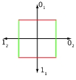
Figure 4.1: 2n = 2-cube

Figure 4.2: 2n = 4-cube

Finally, recall that within the Clifford algebra two vectors are orthogonal if and only if they anti-commute. Hence, if we transform the generating set of $\Gamma_{j}$ linearly,

$$\Gamma_{k}^{\prime}=\sum_{j}T_{jk}\Gamma_{j},$$

the set $\{\Gamma_{1}^{\prime},\ldots,\Gamma_{2n}^{\prime}\}$ satisfies the anti-commutation relations if and only if $(T_{jk})_{jk}$ is an orthogonal matrix. In that case there exists a matching unitary $U(T)$ of ${\cal H}$ which transforms the operator basis as

$$\Gamma_{j}^{\prime}=U(T)\Gamma_{j}U(T)^{\dagger}.$$

We thus have an $\mbox{O}(2n)$ symmetry of the generating set $\Gamma_{1},\ldots,\Gamma_{2n}$. Indeed, this can be extended to a $\mbox{SO}(2n+1)$ symmetry by viewing $\Gamma_{0}$ as an additional ”vector”: It is not difficult to see that $\Gamma_{0}$ anti-commutes with $\Gamma_{1},\ldots,\Gamma_{2n}$. We are thus free to remove one of these operators from the generating set and replace it with $\Gamma_{0}$ to obtain a new set of generators. Evidently, we may also view these as basis vectors. This observation forms the basis of the following little lemma, which allows us to prove our uncertainty relations:

Lemma 4.3.1.

The linear map $\mathbb{P}$ taking $\rho$ as in Eq. (4.3) to

$$\mathbb{P}(\rho):=\frac{1}{d}\left(\mathbb{I}+\sum_{j=0}^{2n}g_{j}\Gamma_{j}\right)$$ (4.4)

is positive. I.e., if $\rho$ is a state, then so is $\mathbb{P}(\rho)$, and in this case $\sum_{j=0}^{2n}g_{j}^{2}\leq 1$. Conversely, if $\sum_{j=0}^{2n}g_{j}^{2}\leq 1$, then

$$\sigma=\frac{1}{d}\left(\mathbb{I}+\sum_{j=0}^{2n}g_{j}\Gamma_{j}\right)$$

is positive semidefinite, hence a state.

Proof 4.3.2.

First, we show that there exists a unitary $U$ such that $\rho^{\prime}=U\rho U^{\dagger}$ has no pseudo-scalar $\Gamma_{0}$, and only one nonzero vector component, say at $\Gamma_{1}$. Hence, our goal is to find the transformation $U$ that rotates $g=\sum_{j=0}^{2n}g_{j}\Gamma_{j}$ to the vector $b=\sqrt{\ell}\Gamma_{1}$, where we let $\ell:=\sum_{j=0}^{2n}g_{j}^{2}=(g_{1}^{\prime})^{2}$. Finding such a transformation for only the first $2n$ generators can easily be achieved, as we saw in Appendix C. The challenge is thus to include $\Gamma_{0}$. To this end we perform three individual operations: First, we rotate $g^{\prime}=\sum_{j=1}^{2n}g_{j}\Gamma_{j}$ onto the vector $b^{\prime}=\sqrt{\ell^{\prime}}\Gamma_{1}$ with $\ell^{\prime}:=\sum_{j=1}^{2n}g_{j}^{2}$. Second, we exchange $\Gamma_{2}$ and $\Gamma_{0}$. And finally we rotate the vector $g^{\prime\prime}=\sqrt{\ell^{\prime}}\Gamma_{1}+g_{0}\Gamma_{2}$ onto the vector $b=\sqrt{\ell}\Gamma_{1}$.

First, we rotate $g^{\prime}=\sum_{j=1}^{2n}g_{j}\Gamma_{j}$ onto the vector $b^{\prime}=\sqrt{\ell^{\prime}}\Gamma_{1}$: This is exactly analogous to the transformation constructed in Appendix C. Consider the vector $\hat{g}=\frac{1}{\sqrt{\ell^{\prime}}}g^{\prime}$ . We have $\hat{g}^{2}=|\hat{g}|^{2}\mathbb{I}=\mathbb{I}$ and thus the vector is of length 1. Let $m=\hat{g}+\Gamma_{1}$ denote the vector lying in the plane spanned by $\Gamma_{1}$ and $\hat{g}$ located exactly halfway between $\Gamma_{1}$ and $\hat{g}$. Let $\hat{m}=c(\hat{g}+\Gamma_{1})$ with $c=1/\sqrt{2(1+g_{1}/\sqrt{\ell^{\prime}})}$. It is easy to verify that $\hat{m}^{2}=\mathbb{I}$ and hence the vector $\hat{m}$ has length 1. To rotate the vector $g^{\prime}$ onto the vector $b^{\prime}$, we now need to first reflect $g^{\prime}$ around the plane perpendicular to $\hat{m}$, and then around the plane perpendicular to $\Gamma_{1}$. Hence, we now define $R=\Gamma_{1}\hat{m}$. Evidently, $R$ is unitary since $RR^{\dagger}=R^{\dagger}R=\mathbb{I}$. First of all, note that

$$Rg^{\prime} = \Gamma_{1}\hat{m}g^{\prime}$$

$$= c\Gamma_{1}\left(\frac{1}{\sqrt{\ell^{\prime}}}g^{\prime}+\Gamma_{1}\right)g^{\prime}$$

$$= c\left(\Gamma_{1}\frac{g^{\prime 2}}{\sqrt{\ell^{\prime}}}+\Gamma_{1}^{2}g^{\prime}\right)$$

$$= c\sqrt{\ell^{\prime}}\left(\Gamma_{1}+\frac{1}{\sqrt{\ell^{\prime}}}g^{\prime}\right)$$

$$= \sqrt{\ell^{\prime}}\hat{m}.$$

Hence,

$$Rg^{\prime}R^{\dagger}=\sqrt{\ell^{\prime}}\hat{m}\hat{m}\Gamma_{1}=\sqrt{\ell^{\prime}}\Gamma_{1}=b^{\prime},$$

as desired. Using the geometry of the Clifford algebra, one can see that $k$-vectors remain $k$-vectors when transformed with the rotation $R$ (see Appendix C). Similarly, it is easy to see that $\Gamma_{0}$ is untouched by the operation $R$

$$R\Gamma_{0}R^{\dagger}=\Gamma_{0}RR^{\dagger}=\Gamma_{0},$$

since $\{\Gamma_{0},\Gamma_{j}\}=0$ for all $j\in\{1,\ldots,2n\}$. We can thus conclude that

$$R\rho R^{\dagger}=\frac{1}{d}\left(\mathbb{I}+\sqrt{\ell^{\prime}}\Gamma_{1}+g_{0}\Gamma_{0}+\sum_{j<k}g^{\prime}_{jk}\Gamma_{jk}+\ldots\right),$$

for some coefficients $g^{\prime}_{jk}$ and similar for the terms involving higher products.

Second, we exchange $\Gamma_{2}$ and $\Gamma_{0}$: To this end, recall that $\Gamma_{2},\ldots,\Gamma_{2n},\Gamma_{0}$ is also a generating set for the Clifford algebra. Hence, we can now view $\Gamma_{0}$ itself as a vector with respect to the new generators. To exchange $\Gamma_{0}$ and $\Gamma_{2}$, we now simply rotate $\Gamma_{0}$ onto $\Gamma_{2}$. Essentially, this corresponds to a rotation about 90 degrees in the plane spanned by vectors $\Gamma_{0}$ and $\Gamma_{2}$. Consider the vector $n=\Gamma_{0}+\Gamma_{2}$ located exactly halfway between both vectors. Let $\hat{n}=n/\sqrt{2}$ be the normalized vector. Let $R^{\prime}=\Gamma_{2}\hat{n}$. A small calculation analogous to the above shows that

$$R^{\prime}\Gamma_{0}R{{}^{\prime\dagger}}=\Gamma_{2}\mbox{ and }R^{\prime}\Gamma_{2}R^{{}^{\prime}\dagger}=-\Gamma_{0}.$$

We also have that $\Gamma_{1}$, $\Gamma_{3},\ldots,\Gamma_{2n}$ are untouched by the operation: for $j\neq 0$ and $j\neq 2$, we have that

$$R^{\prime}\Gamma_{j}R^{{}^{\prime}\dagger}=\Gamma_{j},$$

since $\{\Gamma_{0},\Gamma_{j}\}=\{\Gamma_{2},\Gamma_{j}\}=0$. How does $R^{\prime}$ affect the $k$-vectors in terms of the original generators $\Gamma_{1},\ldots,\Gamma_{2n}$? Using the anti-commutation relations and the definition of $\Gamma_{0}$ it is easy to convince yourself that all $k$-vectors are mapped to $k^{\prime}$-vectors with $k^{\prime}\geq 2$ (except for $\Gamma_{0}$ itself). Hence, the coefficient of $\Gamma_{1}$ remains untouched. We can thus conclude that

$$R^{\prime}R\rho R^{\dagger}R^{{}^{\prime}\dagger}=\frac{1}{d}\left(\mathbb{I}+\sqrt{\ell^{\prime}}\Gamma_{1}+g_{0}\Gamma_{2}+\sum_{j<k}g^{\prime\prime}_{jk}\Gamma_{jk}+\ldots\right),$$

for some coefficients $g^{\prime\prime}_{jk}$ and so on.

Finally, we now rotate the vector $g^{\prime\prime}=\sqrt{\ell^{\prime}}\Gamma_{1}+g_{0}\Gamma_{2}$ onto the vector $b$. Note that $(g^{\prime\prime})^{2}=(\ell+g_{0}^{2})\mathbb{I}=\ell\mathbb{I}$. Let $\hat{g}^{\prime\prime}=g^{\prime\prime}/\sqrt{\ell}$ be the normalized vector. Our rotation is derived exactly analogous to the first step: Let $k=\hat{g}^{\prime\prime}+\Gamma_{1}$, and let $\hat{k}=k/\sqrt{2(1+\sqrt{\ell^{\prime}}/\sqrt{\ell})}$. Let $R^{\prime\prime}=\Gamma_{1}\hat{k}$. A simple calculation analogous to the above shows that

$$R^{\prime\prime}g^{\prime\prime}R^{{}^{\prime\prime}\dagger}=\sqrt{\ell}\Gamma_{1},$$

as desired. Again, we have $R^{\prime\prime}\Gamma_{k}R^{\prime\prime\dagger}=\Gamma_{k}$ for $k\neq 1$ and $k\neq 2$. Furthermore, $k$-vectors remain $k$-vectors under the actions of $R^{\prime\prime}$ [DL03]. Summarizing, we obtain

$$R^{\prime\prime}R^{\prime}R\rho R^{\dagger}R^{{}^{\prime}\dagger}R^{{}^{\prime\prime}\dagger}=\frac{1}{d}\left(\mathbb{I}+\sqrt{\ell}\Gamma_{1}+\sum_{j<k}g^{\prime\prime\prime}_{jk}\Gamma_{jk}+\ldots\right),$$

for some coefficients $g^{\prime\prime\prime}_{jk}$ and so on. Thus, we can take $U=R^{\prime\prime}R^{\prime}R$ to arrive at a new, simpler looking, state

$$\begin{split}\rho^{\prime}&=U\rho U^{\dagger}\\ &=\frac{1}{d}\left(\mathbb{I}+g_{1}^{\prime}\Gamma_{1}+\sum_{j<k}g^{\prime\prime\prime}_{jk}\Gamma_{jk}+\ldots+0\,\Gamma_{0}\right),\end{split}$$

for some $g^{\prime\prime\prime}_{jk}$, etc.

Similarly, there exist of course orthogonal transformations $F_{j}$ that take $\Gamma_{k}$ to $(-1)^{\delta_{jk}}\Gamma_{k}$. Such transformations flip the sign of a chosen Clifford generator. In a similar way to the above, it is easy to see that $F_{j}=\Gamma_{0}\Gamma_{j}$ fulfills this task: we rotate $\Gamma_{j}$ by 90 degrees in the plane given by $\Gamma_{0}$ and $\Gamma_{j}$ as in the example we examined in Appendix C. Now, consider

$$\rho^{\prime\prime}=\frac{1}{2}\left(\rho^{\prime}+F_{j}\rho^{\prime}F_{j}^{\dagger}\right),$$

for $j>1$. Clearly, if $\rho^{\prime}$ was a state, $\rho^{\prime\prime}$ is a state as well. Note that we no longer have terms involving $\Gamma_{j}$ in the basis expansion: Note that if we flip the sign of precisely those terms that have an index $j$ (i.e., they have a factor $\Gamma_{j}$ in the definition of the operator basis), and then the coefficients cancel with those of $\rho^{\prime}$.

We now iterate this map through $j=2,3,\ldots,2n$, and we are left with a final state $\hat{\rho}$ of the form

$$\hat{\rho}=\frac{1}{d}\left(\mathbb{I}+g_{1}^{\prime}\Gamma_{1}\right).$$

By applying $U^{\dagger}=(R^{\prime\prime}R^{\prime}R)^{\dagger}$ from above, we now transform $\hat{\rho}$ to $U^{\dagger}\hat{\rho}U=\mathbb{P}(\rho)$, which is the first part of the lemma.

Looking at $\hat{\rho}$ once more, we see that it can be positive semidefinite only if $g_{1}^{\prime}\leq 1$, i.e., $\sum_{j=0}^{2n}g_{j}^{2}\leq 1$. Evidently, $\mbox{\rm Tr}(\hat{\rho})=1$ and hence $\hat{\rho}$ is a state.

Conversely, if $\sum_{j=0}^{2n}g_{j}^{2}\leq 1$, then the (Hermitian) operator $A=\sum_{j}g_{j}\Gamma_{j}$ has the property

$$A^{2}=\sum_{jk}g_{j}g_{k}\Gamma_{j}\Gamma_{k}=\sum_{j}g_{j}^{2}\mathbb{I}\leq\mathbb{I},$$

i.e. $-\mathbb{I}\leq A\leq\mathbb{I}$, so $\sigma=\frac{1}{d}(\mathbb{I}+A)\geq 0$.

4.3.2 A meta-uncertainty relation

We now first use the above tools to prove a “meta”-uncertainty relation, from which we will then derive two new entropic uncertainty relations. Evidently, we have immediately from the above that

Lemma 4.3.3.

Let $\rho\in\mathcal{H}$ with $\dim\mathcal{H}=2^{n}$ be a quantum state, and consider $K\leq 2n+1$ anti-commuting observables $\Gamma_{j}$. Then,

$$\sum_{j=0}^{K-1}\bigl{(}\mbox{\rm Tr}(\rho\Gamma_{j})\bigr{)}^{2}\leq\sum_{j=0}^{2n}\bigl{(}\mbox{\rm Tr}(\rho\Gamma_{j})\bigr{)}^{2}=\sum_{j=0}^{2n}g_{j}^{2}\leq 1.$$

Our result is essentially a generalization of the Bloch sphere picture to higher dimensions: For $n=1$ ($d=2$) the state is parametrized by $\rho=\frac{1}{2}(\mathbb{I}+g_{1}\Gamma_{1}+g_{2}\Gamma_{2}+g_{0}\Gamma_{0})$ where $\Gamma_{1}=X$, $\Gamma_{2}=Z$ and $\Gamma_{0}=Y$ are the familiar Pauli matrices. Lemma 4.3.3 tells us that $g_{0}^{2}+g_{1}^{2}+g_{2}^{2}\leq 1$, i.e., the state must lie inside the Bloch sphere (see Figure 2.1). Our result may be of independent interest, since it is often hard to find conditions on the coefficients $g_{1},g_{2},\ldots$ such that $\rho$ is a state.

Notice that the $g_{j}=\mbox{\rm Tr}(\rho\Gamma_{j})$ are directly interpreted as the expectations of the observables $\Gamma_{j}$. Indeed, $g_{j}$ is precisely the bias of the $\pm 1$-variable $\Gamma_{j}$:

$$\Pr[\Gamma_{j}=1|\rho]=\frac{1+g_{j}}{2}.$$

Hence, we can interpret Lemma 4.3.3 as a form of uncertainty relation between the observables $\Gamma_{j}$: if one or more of the observables have a large bias (i.e., they are more precisely defined), this limits the bias of the other observables (i.e., they are closer to uniformly distributed).

4.3.3 Entropic uncertainty relations

It turns out that Lemma 4.3.3 has strong consequences for the Rényi and von Neumann entropic averages

$$\frac{1}{K}\sum_{j=0}^{K-1}H_{\alpha}\left(\Gamma_{j}|\rho\right),$$

where $H_{\alpha}(\Gamma_{j}|\rho)$ is the Rényi entropy at $\alpha$ of the probability distribution arising from measuring the state $\rho$ with observable $\Gamma_{j}$. The minima over all states $\rho$ of such expressions can be interpreted as giving entropic uncertainty relations, as we shall now do for $\alpha=2$ (the collision entropy) and $\alpha=1$ (the Shannon entropy).

Theorem 4.3.4.

Let $\dim\mathcal{H}=2^{n}$, and consider $K\leq 2n+1$ anti-commuting observables as defined in Eq. (4.2). Then,

$$\min_{\rho}\frac{1}{K}\sum_{j=0}^{K-1}H_{2}\left(\Gamma_{j}|\rho\right)=1-\log\left(1+\frac{1}{K}\right)\sim 1-\frac{\log e}{K},$$

where $H_{2}(\Gamma_{j}|\rho)=-\log\sum_{b\in\{0,1\}}\mbox{\rm Tr}(\Gamma_{j}^{b}\rho)^{2}$, and the minimization is taken over all states $\rho$. The latter holds asymptotically for large $K$.

Proof 4.3.5.

Using the fact that $\Gamma_{j}^{b}=(\mathbb{I}+(-1)^{b}\Gamma_{j})/2$ we can first rewrite

$$\begin{split}\frac{1}{K}\sum_{j=0}^{K-1}H_{2}\left(\Gamma_{j}|\rho\right)&=-\frac{1}{K}\sum_{j=0}^{K-1}\log\left[\frac{1}{2}\left(1+\mbox{\rm Tr}(\rho\Gamma_{j})^{2}\right)\right]\\ &\geq-\log\left(\frac{1}{2K}\sum_{j=0}^{K-1}\left(1+g_{j}^{2}\right)\right)\\ &\geq 1-\log\left(1+\frac{1}{K}\right),\end{split}$$

where the first inequality follows from Jensen’s inequality and the concavity of the log, and the second from Lemma 4.3.3. Clearly, the minimum is attained if all $g_{j}=\mbox{\rm Tr}(\rho\Gamma_{j})=\sqrt{\frac{1}{K}}$. It follows from Lemma 4.3.1 that our inequality is tight. Via the Taylor expansion of $\log\left(1+\frac{1}{K}\right)$ we obtain the asymptotic result for large $K$.

For the Shannon entropy ($\alpha=1$) we obtain something even nicer:

Theorem 4.3.6.

Let $\dim\mathcal{H}=2^{n}$, and consider $K\leq 2n+1$ anti-commuting observables as defined in Eq. (4.2). Then,

$$\min_{\rho}\frac{1}{K}\sum_{j=0}^{K-1}H(\Gamma_{j}|\rho)=1-\frac{1}{K},$$

where $H(\Gamma_{j}|\rho)=-\sum_{b\in\{0,1\}}\mbox{\rm Tr}(\Gamma_{j}^{b}\rho)\log\mbox{\rm Tr}(\Gamma_{j}^{b}\rho)$, and the minimization is taken over all states $\rho$.

Proof 4.3.7.

To see this, note that by rewriting our objective as above, we observe that we need to minimize the expression

$$\frac{1}{K}\sum_{j=0}^{K-1}H\left(\frac{1\pm\sqrt{t_{j}}}{2}\right),$$

subject to $\sum_{j}t_{j}\leq 1$ and $t_{j}\geq 0$, via the identification $t_{j}=(\mbox{\rm Tr}(\rho\Gamma_{j}))^{2}$. An elementary calculation shows that the function $f(t)=H\left(\frac{1\pm\sqrt{t}}{2}\right)$ is concave in $t\in[0,1]$:

$$f^{\prime}(t)=\frac{1}{4\ln 2}\frac{1}{\sqrt{t}}\bigl{(}\ln(1-\sqrt{t})-\ln(1+\sqrt{t})\bigr{)},$$

and so

$$f^{\prime\prime}(t)=\frac{1}{8\ln 2}\frac{1}{t^{3/2}}\left(\ln\frac{1+\sqrt{t}}{1-\sqrt{t}}-\frac{2\sqrt{t}}{1-t}\right).$$

Since we are only interested in the sign of the second derivative, we ignore the (positive) factors in front of the bracket, and are done if we can show that

$$\begin{split}g(t)&:=\ln\frac{1+\sqrt{t}}{1-\sqrt{t}}-\frac{2\sqrt{t}}{1-t}\\ &=\ln(1+\sqrt{t})+\frac{1}{1+\sqrt{t}}-\ln(1-\sqrt{t})-\frac{1}{1-\sqrt{t}}\end{split}$$

is non-positive for $0\leq t\leq 1$. Substituting $s=1-\sqrt{t}$, which is also between $0$ and $1$, we rewrite this as

$$h(s)=-\ln s-\frac{1}{s}+\ln(2-s)+\frac{1}{2-s},$$

which has derivative

$$h^{\prime}(s)=(1-s)\left(\frac{1}{s^{2}}-\frac{1}{(2-s)^{2}}\right),$$

and this is clearly positive for $0<s<1$. In other words, $h$ increases from its value at $s=0$ (where it is $h(0)=-\infty$) to its value at $s=1$ (where it is $h(1)=0$), so indeed $h(s)\leq 0$ for all $0\leq s\leq 1$. Consequently, also $f^{\prime\prime}(t)\leq 0$ for $0\leq t\leq 1$.

Hence, by Jensen’s inequality, the minimum is attained with one of the $t_{j}$ being $1$ and the others $0$, giving just the lower bound of $1-\frac{1}{K}$.

We have shown that anti-commuting Clifford observables obey the strongest possible uncertainty relation for the von Neumann entropy. It is interesting that in the process of the proof, however, we have found three uncertainty type inequalities (the sum of squares bound, the bound on $H_{2}$, and finally the bound on $H_{1}$), and all three have a different structure of attaining the limit. The sum of squares bound can be achieved in every direction (meaning for every tuple satisfying the bound we get one attaining it by multiplying all components by some appropriate factor), the $H_{2}$ expression requires all components to be equal, while the $H_{1}$ expression demands exactly the opposite.

4.4 Conclusion

We showed that merely choosing our measurements to be mutually unbiased does not lead to strong uncertainty relations. However, we were able to identify another property which does lead to optimal entropic uncertainty relations for two outcome measurements! Anti-commuting Clifford observables obey the strongest possible uncertainty relation for the von Neumann entropy: if we have no uncertainty for one of the measurements, we have maximum uncertainty for all others. We also obtain a slightly suboptimal uncertainty relation for the collision entropy which is strong enough for all cryptographic purposes. Indeed, one could use our entropic uncertainty relation in the bounded quantum storage setting to construct, for example, 1-K oblivious transfer protocols analogous to [DFR⁺07]. Here, instead of encoding a single bit into either the computational or Hadamard basis, which gives us a 1-2 OT, we now encode a single bit into the positive or negative eigenspace of each of these $K$ operators. It is clear from the representation of such operators discussed earlier, that such an encoding can be done experimentally as easily as encoding a single bit into three mutually unbiased basis given by $\sigma_{x}$, $\sigma_{y}$, $\sigma_{z}$. Indeed, our construction can be seen as a direct extension of such an encoding: we obtain the uncertainty relation for the three MUBs previously proved by Sanchez [San93, SR95] as a special case of our analysis for $K=3$. It is perhaps interesting to note that the same operators also play a prominent role in the setting of non-local games as discussed in Chapter 6.3.2.

Sadly, strong uncertainty relations for measurements with more than two outcomes remain inaccessible to us. It has been shown [Feh07] that uncertainty relations for more outcomes can be obtained via a coding argument from uncertainty relations as we construct them here. Yet, these are far from optimal. A natural choice would be to consider the generators of a generalized Clifford algebra, yet such an algebra does not have such nice symmetry properties which enabled us to implement operations on the vector components above. It remains an exciting open question whether such operators form a good generalization, or whether we must continue our search for new properties.

Chapter 5 Locking classical information

Locking classical correlations in quantum states [DHL⁺04] is an exciting feature of quantum information, intricately related to entropic uncertainty relations. In this chapter, we will investigate whether good locking effects can be obtained using mutually unbiased bases.

5.1 Introduction

Consider a two-party protocol with one or more rounds of communication. Intuitively, one would expect that in each round the amount of correlation between the two parties cannot increase by much more than the amount of data transmitted. For example, transmitting $2\ell$ classical bits or $\ell$ qubits (and using superdense coding) should not increase the amount of correlation by more than $2\ell$ bits, no matter what the initial state of the two-party system was. This intuition is accurate when we take the classical mutual information $\mathcal{I}_{c}$ as our correlation measure, and require all communication to be classical. However, when quantum communication was possible at some point during the protocol, everything changes: there exist two-party mixed quantum states, such that transmitting just a single extra bit of classical communication can result in an arbitrarily large increase in $\mathcal{I}_{c}$ [DHL⁺04]. The magnitude of this increase thereby only depends on the dimension of the initial mixed state. Since then similar locking effects have been observed, also for other correlation measures [CW05b, HHHO05]. Such effects play a role in very different scenarios: they have been used to explain physical phenomena related to black holes [SO06], but they are also important in cryptographic applications such as quantum key distribution [KRBM07] and quantum bit string commitment that we will encounter in Chapter 10. We are thus interested in determining how exactly we can obtain locking effects, and how dramatic they can be.

5.1.1 A locking protocol

The correlation measure considered here, is the classical mutual information of a bipartite quantum state $\rho_{AB}$, which is the maximum classical mutual information that can be obtained by local measurements $M_{A}\otimes M_{B}$ on the state $\rho_{AB}$ (see Chapter 2):

$$\mathcal{I}_{c}(\rho_{AB})=\max_{M_{A}\otimes M_{B}}\mathcal{I}(A,B).$$ (5.1)

Recall from Chapter 2 that the mutual information is defined as $\mathcal{I}(A,B)=H(P_{A})+H(P_{B})-H(P_{AB})$ where $H$ is the Shannon entropy. $P_{A}$, $P_{B}$, and $P_{AB}$ are the probability distributions corresponding to the individual and joint outcomes of measuring the state $\rho_{AB}$ with $M_{A}\otimes M_{B}$. The mutual information between $A$ and $B$ is a measure of the information that $B$ contains about $A$. This measure of correlation is of particular relevance for quantum bit string commitments in Chapter 10. Furthermore, the first locking effect was observed for this quantity in the following protocol between two parties: Alice (A) and Bob (B). Let $\mathbb{B}=\{\mathcal{B}_{1},\ldots,\mathcal{B}_{m}\}$ with $\mathcal{B}_{t}=\{|b^{t}_{1}\rangle,\ldots,|b^{t}_{d}\rangle\}$ be a set of $m$ MUBs in $\mathbb{C}^{d}$. Alice picks an element $k\in\{1,\ldots,d\}$ and a basis $\mathcal{B}_{t}\in\mathbb{B}$ uniformly at random. She then sends $|b^{t}_{k}\rangle$ to Bob, while keeping $t$ secret. Such a protocol gives rise to the joint state

$$\rho_{AB}=\frac{1}{md}\sum_{k=1}^{d}\sum_{t=1}^{m}(|k\rangle\langle k|\otimes|t\rangle\langle t|)_{A}\otimes(|b_{k}^{t}\rangle\langle b^{t}_{k}|)_{B}.$$

Clearly, if Alice told her basis choice $t$ to Bob, he could measure in the right basis and obtain the correct $k$. Alice and Bob would then share $\log d+\log m$ bits of correlation, which is also their mutual information $\mathcal{I}_{c}(\sigma_{AB})$, where $\sigma_{AB}$ is the state obtained from $\rho_{AB}$ after the announcement of $t$. But, how large is $\mathcal{I}_{c}(\rho_{AB})$, when Alice does not announce $t$ to Bob? It was shown [DHL⁺04] that in dimension $d=2^{n}$, using the two MUBs given by the unitaries $U_{+}=\mathbb{I}^{\otimes n}$ and $U_{\times}=H^{\otimes n}$ applied to the computational basis we have $\mathcal{I}_{c}(\rho_{AB})=(1/2)\log d$ (see Figure 5.1, where $|x_{b}\rangle=U_{b}|x\rangle$). This means that the single bit of basis information Alice transmits to Bob “unlocks” $(1/2)\log d$ bits: without this bit, the mutual information is $(1/2)\log d$, but with this bit it is $\log d+1$.

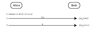
Figure 5.1: A locking protocol for 2 bases.

To get a good locking protocol, we want to use only a small number of bases, i.e., $m$ should be as small as possible, while at the same time forcing $\mathcal{I}_{c}(\rho_{AB})$ to be as low as possible. That is, we want $\log m/(\log d-\mathcal{I}_{c}(\rho_{AB}))$ to be small.

It is also known that if Alice and Bob randomly choose a large set of unitaries from the Haar measure to construct $\mathbb{B}$, then $\mathcal{I}_{c}(\rho_{AB})$ can be brought down to a small constant [HLSW04]. However, no explicit constructions with more than two bases are known that give good locking effects. Based on numerical studies for spaces of prime dimension $3\leq d\leq 30$, one might hope that adding a third MUB would strengthen the locking effect and give $\mathcal{I}_{c}(\rho_{AB})\approx(1/3)\log d$ [DHL⁺04].

Here, however, we show that this intuition fails us. We prove that for three MUBs given by $\mathbb{I}^{\otimes n}$, $H^{\otimes n}$, and $K^{\otimes n}$ where $K=(\mathbb{I}+i\sigma_{x})/\sqrt{2}$ and dimension $d=2^{n}$ for some even integer $n$, we have

$$\mathcal{I}_{c}(\rho_{AB})=\frac{1}{2}\log d,$$ (5.2)

the same locking effect as with two MUBs. We also show that for any subset of the MUBs based on Latin squares and the MUBs in square dimensions based on generalized Pauli matrices [BBRV02], we again obtain Eq. (5.2), i.e., using two or all $\sqrt{d}$ of them makes no difference at all! Finally, we show that for any set of MUBs $\mathbb{B}$ based on generalized Pauli matrices in any dimension, $\mathcal{I}_{c}(\rho_{AB})=\log d-\min_{|\phi\rangle}(1/|\mathbb{B}|)\sum_{\mathcal{B}\in\mathbb{B}}H(\mathcal{B}||\phi\rangle)$, i.e., it is enough to determine a bound on the entropic uncertainty relation to determine the strength of the locking effect. Although bounds for general MUBs still elude us, our results show that merely choosing the bases to be mutually unbiased is not sufficient and we must look elsewhere to find bases which provide good locking.

5.1.2 Locking and uncertainty relations

We first explain the connection between locking and entropic uncertainty relations. In particular, we will see that for MUBs based on generalized Pauli matrices, we only need to look at such uncertainty relations to determine the exact strength of the locking effect.

In order to determine how large the locking effect is for some set of mutually unbiased bases $\mathbb{B}$, and the shared state

$$\rho_{AB}=\sum_{t=1}^{|\mathbb{B}|}\sum_{k=1}^{d}p_{t,k}(|k\rangle\langle k|\otimes|t\rangle\langle t|)_{A}\otimes(|b^{t}_{k}\rangle\langle b^{t}_{k}|)_{B},$$ (5.3)

we must find the value of $\mathcal{I}_{c}(\rho_{AB})$ or at least a good upper bound. That is, we must find a POVM $M_{A}\otimes M_{B}$ that maximizes Eq. (5.1). Here, $\{p_{t,k}\}$ is a probability distribution over $\mathbb{B}\times[d]$. It has been shown in [DHL⁺04] that we can restrict ourselves to taking $M_{A}$ to be the local measurement determined by the projectors $\{|k\rangle\langle k|\otimes|t\rangle\langle t|\}$. It is also known that we can limit ourselves to take the measurement $M_{B}$ consisting of rank one elements $\{\alpha_{i}|\Phi_{i}\rangle\langle\Phi_{i}|\}$ only [Dav78], where $\alpha_{i}\geq 0$ and $|\Phi_{i}\rangle$ is normalized. Maximizing over $M_{B}$ then corresponds to maximizing Bob’s accessible information as defined in Chapter 2 for the ensemble $\mathcal{E}=\{p_{k,t},|b^{t}_{k}\rangle\langle b^{t}_{k}|\}$

$$\mathcal{I}_{acc}(\mathcal{E})=$$ (5.4)

$$\max_{M_{B}}\left(-\sum_{k,t}p_{k,t}\log p_{k,t}+\right.\left.\sum_{i}\sum_{k,t}p_{k,t}\alpha_{i}\langle\Phi_{i}|\rho_{k,t}|\Phi_{i}\rangle\log\frac{p_{k,t}\langle\Phi_{i}|\rho_{k,t}|\Phi_{i}\rangle}{\langle\Phi_{i}|\mu|\Phi_{i}\rangle}\right),$$

where $\mu=\sum_{k,t}p_{k,t}\rho_{k,t}$ and $\rho_{k,t}=|b^{t}_{k}\rangle\langle b^{t}_{k}|$. Therefore, we have $\mathcal{I}_{c}(\rho_{AB})=\mathcal{I}_{acc}(\mathcal{E})$. As we saw in Chapter 2, maximizing the accessible information is often a very hard task. Nevertheless, for our choice of MUBs, the problem will turn out to be quite easy in the end.

5.2 Locking using mutually unbiased bases

5.2.1 An example

We now determine how well we can lock information using specific sets of mutually unbiased bases. We first consider a very simple example with only three MUBs that provides the intuition behind the remainder of our proof. The three MUBs we consider now are generated by the unitaries $\mathbb{I}$, $H$ and $K=(\mathbb{I}+i\sigma_{x})/\sqrt{2}$ when applied to the computational basis. For this small example, we also investigate the role of the prior over the bases and the encoded basis elements. It turns out that this does not affect the strength of the locking effect positively, i.e., we do not obtain a stronger locking affect using a non-uniform prior. Actually, it is possible to show the same for encodings in many other bases. However, we do not consider this case in full generality as to not obscure our main line of argument.

Lemma 5.2.1.

Let $U_{1}=\mathbb{I}^{\otimes n}$,$U_{2}=H^{\otimes n}$, and $U_{3}=K^{\otimes n}$, and take $k\in\{0,1\}^{n}$ where $n$ is an even integer. Let $\{p_{t}\}$ with $t\in[3]$ be a probability distribution over the set $\mathcal{S}=\{U_{1},U_{2},U_{3}\}$. Suppose that $p_{1},p_{2},p_{3}\leq 1/2$ and let $\{p_{t,k}\}$ with $p_{t,k}=p_{t}/d$ be the joint distribution over $\mathcal{S}\times\{0,1\}^{n}$. Consider the ensemble $\mathcal{E}=\{p_{t}\frac{1}{d},U_{t}|k\rangle\langle k|U_{t}^{\dagger}\}$, then

$$\mathcal{I}_{acc}(\mathcal{E})=\frac{n}{2}.$$

If, on the other hand, there exists a $t\in[3]$ such that $p_{t}>1/2$, then $\mathcal{I}_{acc}(\mathcal{E})>n/2$.

Proof 5.2.2.

We first give an explicit measurement strategy and then prove a matching upper bound on $\mathcal{I}_{acc}$. Consider the Bell basis vectors $|\Gamma_{00}\rangle=(|00\rangle+|11\rangle)/\sqrt{2}$, $|\Gamma_{01}\rangle=(|00\rangle-|11\rangle)/\sqrt{2}$, $|\Gamma_{10}\rangle=(|01\rangle+|10\rangle)/\sqrt{2}$, and $|\Gamma_{11}\rangle=(|01\rangle-|10\rangle)/\sqrt{2}$. Note that we can write for the computational basis

$$|00\rangle = \frac{1}{\sqrt{2}}(|\Gamma_{00}\rangle+|\Gamma_{01}\rangle),$$

$$|01\rangle = \frac{1}{\sqrt{2}}(|\Gamma_{10}\rangle+|\Gamma_{11}\rangle),$$

$$|10\rangle = \frac{1}{\sqrt{2}}(|\Gamma_{10}\rangle-|\Gamma_{11}\rangle),$$

$$|11\rangle = \frac{1}{\sqrt{2}}(|\Gamma_{00}\rangle-|\Gamma_{01}\rangle).$$

The crucial fact to note is that if we fix some $k_{1},k_{2}$, then there exist exactly two Bell basis vectors $|\Gamma_{i_{1}i_{2}}\rangle$ such that $|\langle{\Gamma_{i_{1}i_{2}}}|{k_{1},k_{2}}\rangle|^{2}=1/2$. For the remaining two basis vectors the inner product with $|k_{1},k_{2}\rangle$ will be zero. A simple calculation shows that we can express the two-qubit basis states of the other two mutually unbiased bases analogously: for each two qubit basis state there are exactly two Bell basis vectors such that the inner product is zero and for the other two the inner product squared is $1/2$.

We now take the measurement given by $\{|\Gamma_{i}\rangle\langle\Gamma_{i}|\}$ with $|\Gamma_{i}\rangle=|\Gamma_{i_{1}i_{2}}\rangle\otimes\ldots\otimes|\Gamma_{i_{n-1}i_{n}}\rangle$ for the binary expansion of $i=i_{1}i_{2}\ldots i_{n}$. Fix a $k=k_{1}k_{2}\ldots k_{n}$. By the above argument, there exist exactly $2^{n/2}$ strings $i\in\{0,1\}^{n}$ such that $|\langle{\Gamma_{i}}|{k}\rangle|^{2}=1/2^{n/2}$. Putting everything together, Eq. (LABEL:accessible) now gives us for any prior distribution $\{p_{t,k}\}$ that

$$-\sum_{i}\langle\Gamma_{i}|\mu|\Gamma_{i}\rangle\log\langle\Gamma_{i}|\mu|\Gamma_{i}\rangle-\frac{n}{2}\leq\mathcal{I}_{acc}(\mathcal{E}).$$ (5.5)

For our particular distribution we have $\mu=\mathbb{I}/d$ and thus

$$\frac{n}{2}\leq\mathcal{I}_{acc}(\mathcal{E}).$$

We now prove a matching upper bound that shows that our measurement is optimal. For our distribution, we can rewrite Eq. (LABEL:accessible) for the POVM given by $\{\alpha_{i}|\Phi_{i}\rangle\langle\Phi_{i}|\}$ to

$$\mathcal{I}_{acc}(\mathcal{E}) = \max_{M}\left(\log d+\sum_{i}\frac{\alpha_{i}}{d}\sum_{k,t}p_{t}|\langle\Phi_{i}|U_{t}|k\rangle|^{2}\log|\langle\Phi_{i}|U_{t}|k\rangle|^{2}\right)$$

$$= \max_{M}\left(\log d-\sum_{i}\frac{\alpha_{i}}{d}\sum_{t}p_{t}H(\mathcal{B}_{t}||\Phi_{i}\rangle)\right),$$

for the bases $\mathcal{B}_{t}=\{U_{t}|k\rangle\mid k\in\{0,1\}^{n}\}$.

It follows from Corollary 4.2.2 that $\forall i\in\{0,1\}^{n}$ and $p_{1},p_{2},p_{3}\leq 1/2$

$$(1/2-p_{1})[H(\mathcal{B}_{2}||\Phi_{i}\rangle)+H(\mathcal{B}_{3}||\Phi_{i}\rangle)] +$$

$$(1/2-p_{2})[H(\mathcal{B}_{1}||\Phi_{i}\rangle)+H(\mathcal{B}_{3}||\Phi_{i}\rangle)] +$$

$$(1/2-p_{3})[H(\mathcal{B}_{1}||\Phi_{i}\rangle)+H(\mathcal{B}_{2}||\Phi_{i}\rangle)] \geq n/2,$$

where we used the fact that $p_{1}+p_{2}+p_{3}=1$. Reordering the terms we now get $\sum_{t=1}^{3}p_{t}H(\mathcal{B}_{t}||\Phi_{i}\rangle)\geq n/2.$ Putting things together and using the fact that $\sum_{i}\alpha_{i}=d$, we obtain

$$\mathcal{I}_{acc}(\mathcal{E})\leq\frac{n}{2},$$

from which the result follows.

If, on the other hand, there exists a $t\in[3]$ such that $p_{t}>1/2$, then by measuring in the basis $\mathcal{B}_{t}$ we obtain $\mathcal{I}_{acc}(\mathcal{E})\geq p_{t}n>n/2$, since the entropy will be 0 for basis $\mathcal{B}_{t}$ and we have $\sum_{t}p_{t}=1$.

Above, we have only considered a non-uniform prior over the set of bases. In Chapter 3, we observed that when we want to guess the XOR of a string of length $2$ encoded in one (unknown to us) of these three bases, the uniform prior on the strings is not the one that gives the smallest probability of success. This might lead one to think that a similar phenomenon could be observed in the present setting, i.e., that one might obtain better locking with three basis for a non-uniform prior on the strings. In what follows, however, we show that this is not the case.

Let $p_{t}=\sum_{k}p_{k,t}$ be the marginal distribution on the basis, then the difference in Bob’s knowledge between receiving only the quantum state and receiving the quantum state and the basis information, where we will ignore the basis information itself, is given by

$$\Delta(p_{k,t})=H(p_{k,t})-\mathcal{I}_{acc}(\mathcal{E})-H(p_{t}),$$

Consider the post-measurement state $\nu=\sum_{i}\langle\Gamma_{i}|\mu|\Gamma_{i}\rangle|\Gamma_{i}\rangle\langle\Gamma_{i}|$. Using Eq. (5.5) we obtain

$$\Delta(p_{k,t})\leq H(p_{k,t})-S(\nu)+n/2-H(p_{t}),$$ (5.6)

where $S$ is the von Neumann entropy. Consider the state

$$\rho_{12}=\sum_{k=1}^{d}\sum_{t=1}^{3}p_{k,t}(|t\rangle\langle t|)_{1}\otimes(U_{t}|k\rangle\langle k|U_{t}^{\dagger})_{2},$$

for which we have that

$$S(\rho_{12})=H(p_{k,t}) \leq S(\rho_{1})+S(\rho_{2})$$

$$=H(p_{t})+S(\mu)$$

$$\leq H(p_{t})+S(\nu).$$

Using Eq. (5.6) and the previous equation we get

$$\Delta(p_{k,t})\leq n/2,$$

for any prior distribution. This bound is saturated by the uniform prior and therefore we conclude that the uniform prior results in the largest gap possible.

5.2.2 MUBs from generalized Pauli matrices

We now consider MUBs based on the generalized Pauli matrices $X_{d}$ and $Z_{d}$ as described in Chapter 2.4.2. We consider a uniform prior over the elements of each basis and the set of bases. Choosing a non-uniform prior does not lead to a better locking effect.

Lemma 5.2.3.

Let $\mathbb{B}=\{\mathcal{B}_{1},\ldots,\mathcal{B}_{m}\}$ be any set of MUBs constructed on the basis of generalized Pauli matrices in a Hilbert space of prime power dimension $d=p^{N}$. Consider the ensemble $\mathcal{E}=\{\frac{1}{dm},|b^{t}_{k}\rangle\langle b^{t}_{k}|\}$. Then

$$\mathcal{I}_{acc}(\mathcal{E})=\log d-\frac{1}{m}\min_{|\psi\rangle}\sum_{\mathcal{B}_{t}\in\mathbb{B}}H(\mathcal{B}_{t}||\psi\rangle).$$

Proof 5.2.4.

We can rewrite Eq. (LABEL:accessible) for a POVM $M_{B}$ of the form $\{\alpha_{i}|\Phi_{i}\rangle\langle\Phi_{i}|\}$ as

$$\mathcal{I}_{acc}(\mathcal{E}) = \max_{M_{B}}\left(\log d+\sum_{i}\frac{\alpha_{i}}{dm}\sum_{k,t}|\langle{\Phi_{i}}|{b^{t}_{k}}\rangle|^{2}\log|\langle{\Phi_{i}}|{b^{t}_{k}}\rangle|^{2}\right)$$

$$= \max_{M_{B}}\left(\log d-\sum_{i}\frac{\alpha_{i}}{d}\sum_{t}p_{t}H(\mathcal{B}_{t}||\Phi_{i}\rangle)\right).$$

For convenience, we split up the index $i$ into $i=a,b$ with $a=a_{1},\ldots,a_{N}$ and $b=b_{1},\ldots,b_{N}$, where $a_{\ell},b_{\ell}\in\{0,\ldots,p-1\}$ in the following.

We first show that applying generalized Pauli matrices to the basis vectors of a MUB merely permutes those vectors.

Claim 1.

Let $\mathcal{B}_{t}=\{|b^{t}_{1}\rangle,\ldots,|b^{t}_{d}\rangle\}$ be a basis based on generalized Pauli matrices (Chapter 2.4.2) with $d=p^{N}$. Then $\forall a,b\in\{0,\ldots,p-1\}^{N},\forall k\in[d]$ we have that $\exists k^{\prime}\in[d],$ such that $|b^{t}_{k^{\prime}}\rangle=X_{d}^{a_{1}}Z_{d}^{b_{1}}\otimes\ldots\otimes X_{d}^{a_{N}}Z_{d}^{b_{N}}|b^{t}_{k}\rangle$.

Proof 5.2.5.

Let $\mathcal{T}_{p}^{i}$ for $i\in\{0,1,2,3\}$ denote the generalized Pauli’s $\mathcal{T}_{p}^{0}=\mathbb{I}_{p}$, $\mathcal{T}_{p}^{1}=X_{p}$, $\mathcal{T}_{p}^{3}=Z_{p}$, and $\mathcal{T}_{p}^{2}=X_{p}Z_{p}$. Note that $X_{p}^{u}Z_{p}^{v}=\omega^{uv}Z_{p}^{v}X_{p}^{u}$, where $\omega=e^{2\pi i/p}$. Furthermore, define $\mathcal{T}_{p}^{i,(x)}=\mathbb{I}^{\otimes(x-1)}\otimes\mathcal{T}_{p}^{i}\otimes\mathbb{I}^{N-x}$ to be the Pauli operator $\mathcal{T}_{p}^{i}$ applied to the $x$-th qupit. Recall from Section 2.4.2 that there exist sets of Pauli operators $C_{t}$ such that the basis $\mathcal{B}_{t}$ is the unique simultaneous eigenbasis of the set of operators in $C_{t}$, i.e., for all $k\in[d]$ and $f,g\in[N]$, $|b^{t}_{k}\rangle\in\mathcal{B}_{t}$ and $c_{f,g}^{t}\in C_{t}$, we have $c_{f,g}^{t}|b^{t}_{k}\rangle=\lambda_{k,f,g}^{t}|b^{t}_{k}\rangle\textrm{ for some value }\lambda^{t}_{k,f,g}$. Note that any vector $|v\rangle$ that satisfies this equation is proportional to a vector in $\mathcal{B}_{t}$. To prove that any application of one of the generalized Paulis merely permutes the vectors in $\mathcal{B}_{t}$ is therefore equivalent to proving that $\mathcal{T}^{i,(x)}_{p}|b^{t}_{k}\rangle$ are eigenvectors of $c_{f,g}^{t}$ for any $f,g\in[k]$ and $i\in\{1,3\}$. This can be seen as follows: Note that $c_{f,g}^{t}=\bigotimes_{n=1}^{N}\left(\mathcal{T}^{1,(n)}_{p}\right)^{f_{N}}\left(\mathcal{T}^{3,(n)}_{p}\right)^{g_{N}}$ for $f=(f_{1},\ldots,f_{N})$ and $g=(g_{1},\ldots,g_{N})$ with $f_{N},g_{N}\in\{0,\ldots,p-1\}$ [BBRV02]. A calculation then shows that

$$c_{f,g}^{t}\mathcal{T}^{i,(x)}_{p}|b^{t}_{k}\rangle=\tau_{f_{x},g_{x},i}\lambda_{k,f,g}^{t}\mathcal{T}^{i,(x)}_{p}|b^{t}_{k}\rangle,$$

where $\tau_{f_{x},g_{x},i}=\omega^{g_{x}}$ for $i=1$ and $\tau_{f_{x},g_{x},i}=\omega^{-f_{x}}$ for $i=3$. Thus $\mathcal{T}^{i,(x)}_{p}|b^{t}_{k}\rangle$ is an eigenvector of $c^{t}_{f,g}$ for all $t,f,g$ and $i$, which proves our claim.

Suppose we are given $|\psi\rangle$ that minimizes $\sum_{\mathcal{B}_{t}\in\mathbb{T}}H(\mathcal{B}_{t}||\psi\rangle)$. We can then construct a full POVM with $d^{2}$ elements by taking $\{\frac{1}{d}|\Phi_{ab}\rangle\langle\Phi_{ab}|\}$ with $|\Phi_{ab}\rangle=(X_{d}^{a_{1}}Z_{d}^{b_{1}}\otimes\ldots\otimes X_{d}^{a_{N}}Z_{d}^{b_{N}})^{\dagger}|\psi\rangle$. However, it follows from our claim above that $\forall a,b,k,\exists k^{\prime}$ such that $|\langle{\Phi_{ab}}|{b^{t}_{k}}\rangle|^{2}=|\langle{\psi}|{b^{t}_{k^{\prime}}}\rangle|^{2}$, and thus $H(\mathcal{B}_{t}||\psi\rangle)=H(\mathcal{B}_{t}||\Phi_{ab}\rangle)$ from which the result follows.

Determining the strength of the locking effects for such MUBs is thus equivalent to proving bounds on entropic uncertainty relations. We thus obtain as a corollary of Theorem 4.2.4 and Lemma 5.2.3, that, for dimensions which are the square of a prime power (i.e. $d=p^{2N}$), using any product MUBs based on generalized Paulis does not give us any better locking than just using 2 MUBs.

Corollary 5.2.6.

Let $\mathbb{S}=\{\mathcal{S}_{1},\ldots,\mathcal{S}_{m}\}$ with $m\geq 2$ be any set of MUBs constructed on the basis of generalized Pauli matrices in a Hilbert space of prime (power) dimension $s=p^{N}$. Define $U_{t}$ as the unitary that transforms the computational basis into the $t$-th MUB, i.e., $\mathcal{S}_{t}=\{U_{t}|1\rangle,\ldots,U_{t}|s\rangle\}$. Let $\mathbb{B}=\{\mathcal{B}_{1},\ldots,\mathcal{B}_{m}\}$ be the set of product MUBs with $\mathcal{B}_{t}=\{U_{t}\otimes U_{t}^{*}|1\rangle,\ldots,U_{t}\otimes U_{t}^{*}|d\rangle\}$ in dimension $d=s^{2}$. Consider the ensemble $\mathcal{E}=\{\frac{1}{dm},|b^{t}_{k}\rangle\langle b^{t}_{k}|\}$. Then

$$\mathcal{I}_{acc}(\mathcal{E})=\frac{\log d}{2}.$$

Proof 5.2.7.

The claim follows from Theorem 4.2.4 and the proof of Lemma 5.2.3, by constructing a similar measurement formed from vectors $|\hat{\Phi}_{\hat{a}\hat{b}}\rangle=K_{a^{1}b^{1}}\otimes K_{a^{2}b^{2}}^{*}|\psi\rangle$ with $\hat{a}=a^{1}a^{2}$ and $\hat{b}=b^{1}b^{2}$, where $a^{1},a^{2}$ and $b^{1},b^{2}$ are defined like $a$ and $b$ in the proof of Lemma 5.2.3, and $K_{ab}=(X_{d}^{a_{1}}Z_{d}^{b_{1}}\otimes\ldots\otimes X_{d}^{a_{N}}Z^{b_{N}}_{d})^{\dagger}$ from above.

The simple example we considered above is in fact a special case of Corollary 5.2.6. It shows that if the vector that minimizes the sum of entropies has certain symmetries, the resulting POVM can even be much simpler. For example, the Bell states are vectors which such symmetries.

5.2.3 MUBs from Latin squares

At first glance, one might think that maybe the product MUBs based on generalized Paulis are not well suited for locking just because of their product form. Perhaps MUBs with entangled basis vectors do not exhibit this problem? Let’s examine how well MUBs based on Latin squares can lock classical information in a quantum state. All such MUBs are highly entangled, with the exception of the two extra MUBs based on non-Latin squares. Surprisingly, it turns out, however, that any set of at least two MUBs based on Latin squares, does equally well at locking as using just 2 such MUBs. Thus such MUBs perform equally “badly”, i.e., we cannot improve the strength of the locking effect by using more MUBs of this type.

Lemma 5.2.8.

Let $\mathbb{B}=\{\mathcal{B}_{1},\ldots,\mathcal{B}_{m}\}$ with $m\geq 2$ be any set of MUBs in a Hilbert space of dimension $d=s^{2}$ constructed on the basis of Latin squares. Consider the ensemble $\mathcal{E}=\{\frac{1}{dm},|b^{t}_{k}\rangle\langle b^{t}_{k}|\}$. Then

$$\mathcal{I}_{acc}(\mathcal{E})=\frac{\log d}{2}.$$

Proof 5.2.9.

Note that we can again rewrite $\mathcal{I}_{acc}(\mathcal{E})$ as in the proof of Lemma 5.2.3. Consider the simple measurement in the computational basis $\{|i,j\rangle\langle i,j|\mid i,j\in[s]\}$. The result then follows by the same argument as in Lemma 4.2.6.

Intuitively, our measurement outputs one sub-square of the Latin square used to construct the MUBs as depicted in Figure 5.2. As we saw in the construction of MUBs based on Latin squares in Chapter 2.4.1, each entry “occurs” in exactly $\sqrt{d}=s$ MUBs.

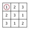
Figure 5.2: Measurement for $|1,1\rangle$.

5.3 Conclusion

We have shown tight bounds on locking for specific sets of mutually unbiased bases. Surprisingly, it turns out that using more mutually unbiased basis does not always lead to a better locking effect. It is interesting to consider what may make these bases so special. The example of three MUBs considered in Lemma 5.2.1 may provide a clue. These three bases are given by the common eigenbases of $\{\sigma_{x}\otimes\sigma_{x},\sigma_{x}\otimes\mathbb{I},\mathbb{I}\otimes\sigma_{x}\}$, $\{\sigma_{z}\otimes\sigma_{z},\sigma_{z}\otimes\mathbb{I},\mathbb{I}\otimes\sigma_{z}\}$ and $\{\sigma_{y}\otimes\sigma_{y},\sigma_{y}\otimes\mathbb{I},\mathbb{I}\otimes\sigma_{y}\}$ respectively [BBRV02]. However, $\sigma_{x}\otimes\sigma_{x}$, $\sigma_{z}\otimes\sigma_{z}$ and $\sigma_{y}\otimes\sigma_{y}$ commute and thus also share a common eigenbasis, namely the Bell basis. This is exactly the basis we will use as our measurement. For all MUBs based on generalized Pauli matrices, the MUBs in prime power dimensions are given as the common eigenbasis of similar sets consisting of strings of Paulis. It would be interesting to determine the strength of the locking effect on the basis of the commutation relations of elements of different sets. Furthermore, perhaps it is possible to obtain good locking from a subset of such MUBs where none of the elements from different sets commute.

It is also worth noting that the numerical results of [DHL⁺04] indicate that at least in dimension $p$ using more than three bases does indeed lead to a stronger locking effect. It would be interesting to know, whether the strength of the locking effect depends not only on the number of bases, but also on the dimension of the system in question.

Whereas general bounds still elude us, we have shown that merely choosing mutually unbiased bases is not sufficient to obtain good locking effects. We thus have to look for different properties. Sadly, whereas we were able to obtain good uncertainty relations in Chapter 4.3, the same approach does not work here: To obtain good locking we must not only find good uncertainty relations, but also find a way to encode many bits using only a small number of encodings.

Part III Entanglement

Chapter 6 Introduction

Entanglement is possibly the most intriguing element of quantum theory. It plays a crucial role in quantum algorithms, quantum cryptography and the understanding of quantum mechanics itself. It enables us to perform quantum teleportation, as well as superdense coding [NC00]. In this part, we investigate one particular aspect of quantum entanglement: the violation of Bell-inequalities, and their implications for classical protocols. But first, let’s take a brief look at the history of entanglement, and introduce the essential ingredients we need later.

6.1 Introduction

In 1935, Einstein, Podolsky and Rosen (EPR) identified one of the striking consequences of what latter became known as entanglement. In their seminal article [EPR35] ”Can Quantum Mechanical Description of Physical Reality Be Considered Complete?” the authors define “elements of reality” as follows:

If, without in any way disturbing a system, we can predict with certainty (i.e. with probability equal to unity) the value of a physical quantity, then there exists an element of physical reality corresponding to this physical quantity.

EPR call a theory that satisfies this condition complete. They put forward the now famous EPR-Paradox, here stated informally using discrete variables as put forward by Bohm [Per93]. EPR assume that if we have a state shared between two spatially separated systems, Alice and Bob, that do not interact at the time of a measurement,

no real change can take place in the second system as a consequence of anything that may be done to the first system.

That means that Alice and Bob cannot use the shared state itself to transmit information. We will also refer to this as the no-signaling condition. Now consider the shared state

$$|\Psi\rangle=\frac{1}{\sqrt{2}}(\underbrace{|0\rangle}_{Alice}\underbrace{|0\rangle}_{Bob}+\underbrace{|1\rangle}_{Alice}\underbrace{|1\rangle}_{Bob})=\frac{1}{\sqrt{2}}(\underbrace{|+\rangle}_{Alice}\underbrace{|+\rangle}_{Bob}+\underbrace{|-\rangle}_{Alice}\underbrace{|-\rangle}_{Bob}).$$ (6.1)

Suppose that we measure Alice’s system in the computational basis to obtain outcome $c_{A}$. Note that we can now predict the outcome of a measurement of Bob’s system in the computational basis with certainty: $c_{B}=c_{A}$, without having disturbed Bob’s system in any way. Thus $c_{B}$ is an “element of physical reality”. However, we might as well have measured Alice’s system in the Hadamard basis to obtain outcome $h_{A}$. Likewise, we can now predict with certainty the outcome of measuring Bob’s system in the Hadamard basis, $h_{B}=h_{A}$, again without causing any disturbance to the second system. Thus $h_{B}$ should also be an “element of physical reality”. But as we saw in Chapter 4, quantum mechanics forbids us to assign exact values to both $c_{B}$ and $h_{B}$ simultaneously, as measurements in the computational and Hadamard basis are non-commutative. Indeed, in Chapter 4.2, we saw that these two measurements give the strongest entropic uncertainty relation for two measurements. EPR thus conclude

that the quantum mechanical description of reality given by the wave function is not complete.

EPR’s article spurred a flurry of discussion that continues up to the present day. Shortly after the publication of their article, Schrödinger published two papers in which he coined the term entanglement (German: Verschränkung) [Sch35b, Sch35a] and investigated this phenomenon which he described as “not one, but rather the characteristic trait of quantum mechanics, the one that enforces its entire departure from classical lines of thought” [Sch35b]. One point of discussion in the ensuing years was whether the fact that quantum mechanics is not complete, means that there might exist a more detailed description of nature which is complete. Even though, these more detailed descriptions also called “hidden variables” had remained inaccessible to us so far: a better theory and better technology might enable us to learn them. Thus quantum mechanical observations would merely appear to be probabilistic in the absence of our knowledge of such hidden variables.

6.1.1 Bell’s inequality

This idea was put to rest by Bell [Bel65] in 1964, when he proposed conditions that any classical theory, i.e. any theory based on local hidden variables, has to satisfy, and which can be verified experimentally. These conditions are known as Bell inequalities. Intuitively, Bell inequalities measure the strength of non-local correlations attainable in any classical theory. Non-local correlations arise as the result of measurements performed on a quantum system shared between two spatially separated parties. Imagine two parties, Alice and Bob, who are given access to a shared quantum state $|\Psi\rangle$, but cannot communicate. In the simplest case, each of them is able to perform one of two possible measurements. Every measurement has two possible outcomes labeled $\pm 1$. Alice and Bob now measure $|\Psi\rangle$ using an independently chosen measurement setting and record their outcomes. In order to obtain an accurate estimate for the correlation between their measurement settings and the measurement outcomes, they perform this experiment independently many times using an identically prepared state $|\Psi\rangle$ in each round.

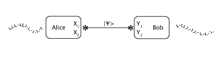
Figure 6.1: Alice and Bob measure many copies of $|\Psi\rangle$

Both classical and quantum theories impose limits on the strength of non-local correlations. In particular, both should not violate the non-signaling condition of special relativity as put forward by EPR above. That is, the local choice of the measurement setting does not allow Alice and Bob to transmit information. Limits on the strength of correlations which are possible in the framework of any classical theory are the Bell inequalities. The best known Bell inequality is the Clauser, Horne, Shimony and Holt (CHSH) inequality [CHSH69]

$$\langle CHSH\rangle_{c}=|\langle X_{1}Y_{1}\rangle+\langle X_{1}Y_{2}\rangle+\langle X_{2}Y_{1}\rangle-\langle X_{2}Y_{2}\rangle|\leq 2,$$ (6.2)

where $X_{1},X_{2}$ and $Y_{1},Y_{2}$ are the observables representing the measurement settings of Alice and Bob respectively and we use $\langle X_{i}Y_{j}\rangle=\langle\Psi|X_{i}\otimes Y_{j}|\Psi\rangle$ to denote the mean value of $X_{i}$ and $Y_{j}$. Quantum mechanics allows for a violation of the CHSH inequality, and is thus indeed non-classical: If we take the shared state $|\Psi\rangle=(|00\rangle+|11\rangle)/\sqrt{2}$ and let $X_{1}=\sigma_{x}$, $X_{2}=\sigma_{z}$, $Y_{1}=(\sigma_{x}+\sigma_{z})/2$, and $Y_{2}=(\sigma_{x}-\sigma_{z})/2$ we obtain

$$\langle CHSH\rangle_{q}=|\langle X_{1}Y_{1}\rangle+\langle X_{1}Y_{2}\rangle+\langle X_{2}Y_{1}\rangle-\langle X_{2}Y_{2}\rangle|=2\sqrt{2}.$$

Most importantly, this violation can be experimentally verified allowing us to test the validity of the theory. The first such tests were performed by Clauser [Cla76] and Aspect, Dalibard, Grangier, and Roger [AGR82, ADR82]. Over the years these tests have been refined considerably, ruling out many loopholes present in the initial experiments such as for example detector inefficiency [RKM⁺01]. Yet, no conclusive test has been achieved so far. Unfortunately, such experimental concerns are outside the scope of this thesis, and we merely point to an overview of such issues [Asp99].

6.1.2 Tsirelson’s bound

Curiously, even quantum mechanics itself still limits the strength of non-local correlations. Tsirelson’s bound [Tsi80] says that for quantum mechanics

$$|\langle X_{1}Y_{1}\rangle+\langle X_{1}Y_{2}\rangle+\langle X_{2}Y_{1}\rangle-\langle X_{2}Y_{2}\rangle|\leq 2\sqrt{2},$$

and thus the above measurements are optimal. We provide a simple proof of this fact in Chapter 7. It is interesting to consider what would happen if quantum mechanics allowed for more powerful non-local correlations. To this end, it is convenient to rewrite the CHSH inequality from Eq. (6.2) in the form

$$\sum_{x,y\in\{0,1\}}\Pr[a_{x}\oplus b_{y}=x\cdot y]\leq 3.$$

Here, $x\in\{0,1\}$ and $y\in\{0,1\}$ denote the choice of Alice’s and Bob’s measurement, $a_{x}\in\{0,1\}$ and $b_{y}\in\{0,1\}$ the respective binary outcomes, and $\oplus$ addition modulo $2$ (see Section 6.2.3 for details). In this form, quantum mechanics allows a violation up to the maximal value of $2+\sqrt{2}$. Since special relativity would even allow a violation of Tsirelson’s bound, Popescu and Rohrlich [PR94, PR96, PR97] raised the question why nature is not more ’non-local’? That is, why does quantum mechanics not allow for a stronger violation of the CHSH inequality up to the maximal value of 4? To gain more insight into this question, they constructed a toy-theory based on non-local boxes. Each such box takes inputs $x,y\in\{0,1\}$ from Alice and Bob respectively and always outputs measurement outcomes $a_{x}$,$b_{y}$ such that $x\cdot y=a_{x}\oplus b_{y}$. Alice and Bob still cannot use this box to transmit any information. However, since for all $x$ and $y$, $\Pr[a_{x}\oplus b_{y}=x\cdot y]=1$, the above sum equals 4 and thus non-local boxes lead to a maximum violation of the CHSH inequality.

Van Dam [vD05, vD00] has shown that having access to such non-local boxes allows Alice and Bob to perform any kind of distributed computation by transmitting only a single bit of information. This is even true for slightly less perfect boxes achieving weaker correlations [BBL⁺06]. In [BCU⁺06], we showed that given any non-local boxes, Alice and Bob could perform bit commitment and oblivious transfer, which is otherwise known to be impossible. Thus, such cryptographic principles are in principle compatible with the theory of non-signaling: non-signaling itself does not prevent us from implementing them.

Looking back to the uncertainty relations in Chapter 4, which rest at the heart of the EPR paradox, we might suspect that the violation of the CHSH inequality likewise depends on the commutation relations between the local measurements of Alice and Bob. Indeed, it has been shown by Landau [Lan87], and Khalfin and Tsirelson [KT87], there exists a state $|\Psi\rangle$ such that

$$|\langle X_{1}Y_{1}\rangle+\langle X_{1}Y_{2}\rangle+\langle X_{2}Y_{1}\rangle-\langle X_{2}Y_{2}\rangle|=2\sqrt{1+4\mbox{$\parallel{[X_{1}^{0},X_{2}^{0}][Y_{1}^{0},Y_{2}^{0}]}\parallel$}},$$

for any $X_{1}=X_{1}^{0}-X_{1}^{1}$, $X_{2}=X_{2}^{0}-X_{2}^{1}$ and $Y_{1}=Y_{1}^{0}-Y_{1}^{1}$, $Y_{2}=Y_{2}^{0}-Y_{2}^{1}$, where we use the superscripts ’0’ and ’1’ to denote the projectors onto the positive and negative eigenspace respectively. Thus, given any observables $X_{1},X_{2}$ and $Y_{1},Y_{2}$, the CHSH inequality is violated if and only if $[X_{1}^{0},X_{2}^{0}][Y_{1}^{0},Y_{2}^{0}]\neq 0$.

6.2 Setting the stage

6.2.1 Entangled states

The state given in Eq. (6.1) is just one possible example of an entangled state. Recall from Chapter 2 that if $|\Psi\rangle\in\mathcal{H}^{A}\otimes\mathcal{H}^{B}$ is a pure state, we say that $|\Psi\rangle$ is separable if and only if there exist states $|\Psi^{A}\rangle\in\mathcal{H}^{A}$ and $|\Psi^{B}\rangle\in\mathcal{H}^{B}$ such that $|\Psi\rangle=|\Psi^{A}\rangle\otimes|\Psi^{B}\rangle$. A separable pure state is also called a product state. A state that is not separable is called entangled. For mixed states the definition is slightly more subtle. Let $\rho\in\mathcal{S}(\mathcal{H}^{A}\otimes\mathcal{H}^{B})$ be a mixed state. Then $\rho$ is called a product state if there exist $\rho^{A}\in\mathcal{S}(\mathcal{H}^{A})$ and $\rho^{B}\in\mathcal{S}(\mathcal{H}^{B})$ such that $\rho=\rho^{A}\otimes\rho^{B}$. The state $\rho$ is called separable, if there exists an ensemble $\mathcal{E}=\{p_{j},|\Psi_{j}\rangle\langle\Psi_{j}|\}$ such that $|\Psi_{j}\rangle=|\Psi_{j}^{A}\rangle\otimes|\Psi_{j}^{B}\rangle$ with $|\Psi_{j}^{A}\rangle\in\mathcal{H}^{A}$ and $|\Psi_{j}^{B}\rangle\in\mathcal{H}^{B}$ for all $j$, such that

$$\rho=\sum_{j}p_{j}|\Psi_{j}\rangle\langle\Psi_{j}|=\sum_{j}p_{j}|\Psi_{j}^{A}\rangle\langle\Psi_{j}^{A}|\otimes|\Psi_{j}^{B}\rangle\langle\Psi_{j}^{B}|.$$

Intuitively, if $\rho$ is separable then $\rho$ corresponds to a mixture of separable pure states according to a joint probability distribution $\{p_{j}\}$, a purely classical form of correlation. Given a description of a mixed state $\rho$ it is an NP-hard problem to decide whether $\rho$ is separable [Gur03]. However, many criteria and approximation algorithms have been proposed [DPS02, DPS04, DPS05, IT06, ITCE04]. It is an interesting question to determine the maximal violation of a given Bell-inequality for a fixed state $\rho$ [LD07]. Here, we only concern ourselves with maximal violations of Bell inequalities, and refer to [Ioa07] for an overview of the separability problem. Generally, the maximal violation is obtained by using the maximally entangled state. However, there are cases for which the maximal violation is achieved by a non maximally entangled state [CGL⁺02]. Note that we can never observe a Bell inequality violation for a separable state: it is no more than a classical mixture of separable pure states. On the other hand, any two-qubit pure state that is entangled violates the CHSH inequality [Gis91]. However, not all entangled mixed states violate the CHSH inequality! A counterexample was given by Werner [Wer81] with the so-called Werner-state

$$\rho_{W}=p\frac{2}{d^{2}+d}P_{sym}+(1-p)\frac{2}{d^{2}-d}P_{asym},$$

where $P_{sym}$ and $P_{asym}$ are projectors onto the symmetric and the anti-symmetric subspace respectively. For $p\geq 1/2$ this state is separable, but it is entangled for $p<1/2$. Yet, the CHSH inequality is not violated. A lot of work has been done to quantify the amount of entanglement in quantum states, and we refer to [Ter99, Eis01, Chr05] for an overview.

6.2.2 Other Bell inequalities

The CHSH inequality we encountered above is by no means the only Bell inequality. Recall that non-local correlations arise as the result of measurements performed on a quantum system shared between two spatially separated parties. Let $x$ and $y$ be the variables corresponding to Alice and Bob’s choice of measurement. Let $a$ and $b$ denote the corresponding outcomes. Let $\Pr[a,b|x,y]$ be the probability of obtaining outcomes $a,b$ given settings $x,y$. What values are allowed for $\Pr[a,b|x,y]$? Clearly, we want that for all $x,y,a,b$ we have that $\Pr[a,b|x,y]\geq 0$ and $\sum_{a,b}\Pr[a,b|x,y]=1$. From the no-signaling condition we furthermore obtain that the marginals obey $\Pr[a|x]=\Pr[a|x,y]=\sum_{b}\Pr[a,b|x,y]$ and likewise for $\Pr[b|y]$, i.e. the probability of Alice’s measurement outcome is independent of Bob’s choice of measurement setting, and vice versa. For $n$ players, who each perform one of $N$ measurements with $k$ possible outcomes, we have $(Nk)^{n}$ such probabilities to assign, giving us a $(Nk)^{n}$ dimensional vector. To find all Bell inequalities, we now look for inequalities that bound the classically accessible region (a convex polytope) for such assignments. It is clear that we can find a huge number of such inequalities. Of course, often the most interesting inequalities are the ones that are satisfied only classically, but where we can find a better quantum strategy. Much work has been done to identify such inequalities, and we refer to [WW01b] for an excellent overview. In the following chapters, we are interested in the following related question: Given an inequality, what is the optimal quantum measurement strategy that maximizes the inequality?

6.2.3 Non-local games

It is often convenient to view Bell experiments as a game between two, or more, distant players, who cooperate against a special party. We call this special party the verifier. In a two player game with players Alice and Bob, the verifier picks two questions, say $s_{1}$ and $s_{2}$, and hands them to Alice and Bob respectively, who now need to decide answers $a_{1}$ and $a_{2}$. To this end, they may agree on any strategy beforehand, but can no longer communicate once the game starts. The verifier then decides according to a fixed set of public rules, whether Alice and Bob win by giving answers $a_{1},a_{2}$ to questions $s_{1},s_{2}$. In a quantum game, Alice and Bob may perform measurements on a shared entangled state to determine their answers. We can thus think of the questions as measurement settings and the answers as measurement outcomes.

More formally, we consider games among $N$ players $P_{1},\ldots,P_{N}$. Let $S_{1},\ldots,S_{N}$ and $A_{1},\ldots,A_{N}$ be finite sets corresponding to the possible questions and answers respectively. Let $\pi$ be a probability distribution on $S_{1}\times\ldots\times S_{N}$, and let $V$ be a predicate on $A_{1}\times\ldots\times A_{N}\times S_{1}\times\ldots\times S_{N}$. Then $G=G(V,\pi)$ is the following $N$-player cooperative game: A set of questions $(s_{1},\ldots,s_{N})\in S_{1}\times\ldots\times S_{N}$ is chosen at random according to the probability distribution $\pi$. Player $P_{j}$ receives question $s_{j}$, and then responds with answer $a_{j}\in A_{j}$. The players win if and only if $V(a_{1},\ldots,a_{N},s_{1},\ldots,s_{N})=1$. We write $V(a_{1},\ldots,a_{N}|s_{1},\ldots,s_{N})=V(a_{1},\ldots,a_{N},s_{1},\ldots,s_{N})$ to emphasize the fact that $a_{1},\ldots,a_{N}$ are the answers given questions $s_{1},\ldots,s_{N}$.

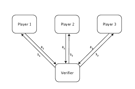
Figure 6.2: Multiplayer non-local games.

The value of the game $\omega(G)$ is the probability that the players win the game, maximized over all possible strategies. We use $\omega_{c}(G)$ and $\omega_{q}(G)$ to differentiate between the value of the game in the classical and quantum case respectively. Classically, $\omega_{c}(G)$ can always be attained by a deterministic strategy [CHTW04a]. We can thus write

$$\omega_{c}(G)=\max_{f_{1},\ldots,f_{N}}\sum_{s_{1},\ldots,s_{N}}\pi(s_{1},\ldots,s_{N})V(f_{1}(s_{1}),\ldots,f_{N}(s_{N})|s_{1},\ldots,s_{N}),$$ (6.3)

where the maximization is taken over all functions $f_{j}:S_{j}\rightarrow A_{j}$ that determine answers $a_{j}=f_{j}(s_{j})$.

Quantumly, the strategy of the players consists of their choice of measurements and shared entangled state. Let $|\Psi\rangle$ denote the players’ choice of state, and let $X_{s_{j}}^{[j]}=\{X_{s_{j}}^{a_{j},[j]}\mid a_{j}\in A_{j}\}$ denote the POVM of player $P_{j}$ for question $s_{j}\in S_{j}$. Here, we always assume that the underlying Hilbert space is finite-dimensional. The value of the quantum game is then

$$\omega_{q}(G)=\max_{X^{[1]},\ldots,X^{[N]}}\sum_{s_{1},\ldots,s_{N}}\pi(s_{1},\ldots,s_{N})\sum_{a_{1},\ldots,a_{N}}\langle\Psi|X_{s_{1}}^{a_{1},[1]}\otimes\ldots\otimes X_{s_{N}}^{a_{N},[N]}|\Psi\rangle,$$ (6.4)

where the maximization is taken over all POVMS $X_{s_{j}}^{[j]}$ for all $j\in[N]$ and $s_{j}\in S_{j}$. In the following, we say that a set of measurement operators achieves $p$, if

$$p=\sum_{s_{1},\ldots,s_{N}}\pi(s_{1},\ldots,s_{N})\sum_{a_{1},\ldots,a_{N}}\langle\Psi|X_{s_{1}}^{a_{1},[1]}\otimes\ldots\otimes X_{s_{N}}^{a_{N},[N]}|\Psi\rangle.$$

Of particular relevance in the next chapters is a special class of two-player games known as XOR-games [CHTW04a]: Here, $N=2$ and we assume that $A_{1}=A_{2}=\{0,1\}$. The two players $P_{1}$ (Alice) and $P_{2}$ (Bob) each have only two possible measurement outcomes. Furthermore, the winning condition only depends on the XOR of answers $a_{1}$ and $a_{2}$ and thus we write $V(c|s_{1},s_{2})$ with $c=a_{1}\oplus a_{2}$. It can be shown [CHTW04a] that the optimal POVM in this case consists only of projectors. We can thus write $X_{s_{1}}^{[1]}$ and $X_{s_{2}}^{[2]}$ as observables with two eigenvalues: $X_{s_{1}}^{[1]}=X_{s_{1}}^{0,[1]}-X_{s_{1}}^{1,[1]}$ and $X_{s_{2}}^{[2]}=X_{s_{2}}^{0,[2]}-X_{s_{2}}^{1,[2]}$ where $s_{1}\in S_{1}$ and $s_{2}\in S_{2}$. A small calculation using the fact that $X_{s_{1}}^{0,[1]}+X_{s_{1}}^{1,[1]}=\mathbb{I}$ and $X_{s_{2}}^{0,[2]}+X_{s_{2}}^{1,[2]}=\mathbb{I}$ shows that we can rewrite the optimal value of a quantum XOR-game as

$$\omega_{q}(G)=$$ (6.5)

$$\max_{X^{[1]},X^{[2]}}\frac{1}{2}\sum_{s_{1},s_{2}}\pi(s_{1},s_{2})\sum_{c\in\{0,1\}}V(c|s_{1},s_{2})(1+(-1)^{c}\langle\Psi|X_{s_{1}}^{[1]}\otimes X_{s_{2}}^{[2]}|\Psi\rangle).$$ (6.6)

From the above, we can see that XOR-games correspond to correlation inequalities with two-outcome measurements. We will see in Chapter 7 that this reformulation enables us to determine the optimal measurements for such XOR-games in a very simple manner. Indeed, the CHSH inequality can be rephrased as a simple quantum XOR-game. Here, Alice and Bob win if and only if given questions $s_{1},s_{2}$ they return answers $a_{1},a_{2}$ such that $s_{1}\cdot s_{2}=a_{1}\oplus a_{2}$, i.e. we have $V(c|s_{1},s_{2})=1$ if and only if $s_{1}\cdot s_{2}=c$. Recalling Eq. (6.2) we can write

$$\omega(CHSH)=\frac{1}{2}\left(1+\frac{\langle CHSH\rangle}{4}\right),$$

from which we obtain $\omega_{q}(CHSH)=1/2+1/(2\sqrt{2})$ vs. $\omega_{c}(CHSH)=3/4$.

6.3 Observations

In the following chapters, we are concerned with finding the optimal quantum measurement strategies for Bell inequalities. To this end, we first make a few simple observations that help us understand the structural properties of our problem. In particular, this also enables us to understand the relation between Bell inequalities and the problem of post-measurement information in Chapter 6.4. We then present a theorem by Tsirelson [Tsi80, Tsi87] that plays a crucial role in the subsequent chapters.

6.3.1 Simple structural observations

Suppose we are given a set of measurements for Alice and Bob and a shared state $\rho$. Can we reduce the dimension of Alice and Bob’s measurements operators and the thereby amount of entanglement they need? As we saw in Chapter 2, we can often simplify our problem by identifying its classical and quantum part. Indeed, this is also the case here.

Lemma 6.3.1.

Let $\mathcal{H}=\mathcal{H}^{A}\otimes\mathcal{H}^{B}$ and let $\mathcal{A}=\{X_{s}^{a}\in\mathbb{B}(\mathcal{H}^{A})\}$ and $\mathcal{B}=\{Y_{t}^{b}\in\mathbb{B}(\mathcal{H}^{B})\}$ be the set of Alice and Bob’s measurement operators respectively. Let $\rho\in\mathcal{S}(\mathcal{H})$ be the state shared by Alice and Bob. Suppose that for such operators we have

$$q=\sum_{s\in S,t\in T}\pi(s,t)\sum_{a\in A,b\in B}V(a,b|s,t)\mbox{\rm Tr}(X_{s}^{a}\otimes Y_{t}^{b}\rho).$$

Then there exist measurement operators $\tilde{\mathcal{A}}=\{\tilde{X}_{s}^{a}\}$ and $\tilde{\mathcal{B}}=\{\tilde{Y}_{t}^{b}\}$ and a state $\tilde{\rho}$ such

$$q\leq\sum_{s\in S,t\in T}\pi(s,t)\sum_{a\in A,b\in B}V(a,b|s,t)\mbox{\rm Tr}(\tilde{X}_{s}^{a}\otimes\tilde{Y}_{t}^{b}\tilde{\rho}).$$

and the $C^{*}$-algebra generated by $\tilde{\mathcal{A}}$ and $\tilde{\mathcal{B}}$ is simple.

Proof 6.3.2.

Let $\mathscr{A}=\langle\mathcal{A}\rangle$ and $\mathscr{B}=\langle\mathcal{B}\rangle$. If $\mathscr{A}$ and $\mathscr{B}$ are simple, we are done. If not, we know from Lemma B.4.1 and Lemma B.4.5 that there exists a decomposition $\mathcal{H}^{A}\otimes\mathcal{H}^{B}=\bigoplus_{jk}\mathcal{H}^{A}_{j}\otimes\mathcal{H}^{B}_{k}$. Consider $\mbox{\rm Tr}((M^{A}\otimes M^{B})\rho)$, where $M^{A}\otimes M^{B}\in\mathscr{A}\otimes\mathscr{B}$. It follows from the above that $M^{A}\otimes M^{B}=\bigoplus_{jk}(\Pi^{A}_{j}\otimes\Pi^{B}_{k})M^{A}\otimes M^{B}(\Pi^{A}_{j}\otimes\Pi^{B}_{k})$, where $\Pi^{A}_{j}$ and $\Pi^{B}_{k}$ are projectors onto $\mathcal{H}^{A}_{j}$ and $\mathcal{H}^{B}_{k}$ respectively. Let $\hat{\rho}=\bigoplus_{jk}(\Pi^{A}_{j}\otimes\Pi^{B}_{k})\rho(\Pi^{A}_{j}\otimes\Pi^{B}_{k})$. Clearly,

$$\mbox{\rm Tr}((M^{A}\otimes M^{B})\hat{\rho}) = \sum_{jk}\mbox{\rm Tr}\left((\Pi^{A}_{j}\otimes\Pi^{B}_{k})M^{A}\otimes M^{B}(\Pi^{A}_{j}\otimes\Pi^{B}_{k})\rho\right)$$

$$= \mbox{\rm Tr}((M^{A}\otimes M^{B})\rho).$$

The statement now follows immediately by convexity: Alice and Bob can now measure $\rho$ using $\{\Pi^{A}_{j}\otimes\Pi^{B}_{k}\}$ and record the classical outcomes $j,k$. The new measurements are then $\tilde{A}_{s,j}^{a}=\Pi^{A}_{j}X_{s}^{a}\Pi^{A}_{j}$ and $\tilde{B}_{t,k}^{b}=\Pi^{B}_{k}Y_{t}^{b}\Pi^{B}_{k}$ on state $\tilde{\rho}_{jk}=(\Pi^{A}_{j}\otimes\Pi^{B}_{k})\rho(\Pi^{A}_{j}\otimes\Pi^{B}_{k})/\mbox{\rm Tr}((\Pi^{A}_{j}\otimes\Pi^{B}_{k})\rho)$. By construction, $\tilde{\mathscr{A}}_{j}=\{\tilde{A}_{s,j}^{a}\}$ and $\tilde{\mathscr{B}}_{k}=\{\tilde{B}_{t,k}^{b}\}$ are simple.

Let $q_{jk}$ denote the probability that we obtain outcomes $j,k$, and let

$$r_{jk}=\sum_{s\in S,t\in T}\pi(s,t)\sum_{a\in A,b\in B}V(a,b|s,t)\mbox{\rm Tr}(\tilde{A}^{a}_{s,j}\otimes\tilde{B}^{b}_{t,j}\tilde{\rho}_{jk}).$$

Then $q=\sum_{jk}q_{jk}r_{jk}\leq\max_{jk}r_{jk}$. Let $u,v$ be such that $r_{u,v}=\max_{jk}r_{jk}$. Hence, we can skip the initial measurement and instead use measurements $\tilde{X}_{s}^{a}=\tilde{A}_{s,u}^{a}$, $\tilde{Y}_{t}^{b}=\tilde{B}_{t,v}^{b}$ and state $\tilde{\rho}=\tilde{\rho}_{u,v}$.

It also follows immediately from the above proof that

Corollary 6.3.3.

$\dim(\tilde{\rho})\leq\dim(\mathcal{H}^{A}_{u})\dim(\mathcal{H}^{B}_{v})$

We can thus assume without loss of generality, that the algebra generated by Alice and Bob’s optimal measurements is always simple. We also immediately see why we can simulate the quantum measurement classically if Alice or Bob’s measurements commute locally. Indeed, the above proof tells us how to construct the appropriate classical strategy:

Corollary 6.3.4.

Let $\mathcal{H}=\mathcal{H}^{A}\otimes\mathcal{H}^{B}$ and let $\mathcal{A}=\{X_{s}^{a}\in\mathbb{B}(\mathcal{H}^{A})\}$ and $\mathcal{B}=\{Y_{t}^{b}\in\mathbb{B}(\mathcal{H}^{B})\}$ be the set of Alice and Bob’s measurement operators respectively. Let $\rho\in\mathcal{S}(\mathcal{H})$ be the state shared by Alice and Bob. Let $p$ be the value of the non-local game achieved using these measurements. Suppose that for all $s,s^{\prime}$,and $a,a^{\prime}$ we have that $[X_{s}^{a},X_{s^{\prime}}^{a^{\prime}}]=0$ (or for all $t,t^{\prime}$, $b,b^{\prime}$ $[Y_{t}^{b},Y_{t^{\prime}}^{b^{\prime}}]=0$). Then there exists a classical strategy for Alice and Bob that achieves $p$.

Proof 6.3.5.

Our conditions imply that either $\mathscr{A}$ or $\mathscr{B}$ is abelian. Suppose wlog that $\mathscr{A}$ is abelian. Hence, by the above proof we have $\max_{j}\dim(\mathcal{H}^{A}_{j})=1$. Again, Alice and Bob perform the measurements determined by $\Pi^{A}_{j}$ and $\Pi^{B}_{k}$ and record their outcomes $j,k$. Since $\dim(\mathcal{H}^{A}_{j})=1$, Alice’s post-measurement state is in fact classical, and we have no further entanglement between Alice and Bob.

To violate a Bell inequality, Alice and Bob must thus use measurements which do not commute locally. However, since Alice and Bob are spatially separated, we can write Alice and Bob’s measurement operators as $X=\hat{X}\otimes\mathbb{I}$ and $Y=\mathbb{I}\otimes\hat{Y}$ respectively as for any $\rho$ we can write $\mbox{\rm Tr}(\rho(X\otimes Y))=\mbox{\rm Tr}(\rho(\hat{X}\otimes\mathbb{I})(\mathbb{I}\otimes\hat{Y}))$. Thus $[X,Y]=0$. Thus from a bipartite structure we obtain certain commutation relations. How about the converse? As it turns out, in any finite-dimensional $C^{*}$-algebra, these two notions are equivalent: From commutation we immediately obtain a bipartite structure! We encounter this well-known, rather beautiful observation in Appendix B.

6.3.2 Vectorizing measurements

In Chapter 7, we show how to obtain the optimal measurements for any bipartite correlation inequality. At first sight, this may appear to be a daunting problem: We must simultaneously maximize Eq. (6.5) over the state $\rho$ as well as measurement operators of the form $X\otimes Y$, a problem which is clearly not convex. Yet, the following brilliant observation by Tsirelson [Tsi80, Tsi87] greatly simplifies our problem.

Theorem 6.3.6 (Tsirelson).

Let $X_{1},\ldots,X_{n}$ and $Y_{1},\ldots,Y_{m}$ be observables with eigenvalues in the interval $[-1,1]$. Then for any state $|\Psi\rangle\in\mathcal{H}^{A}\otimes\mathcal{H}^{B}$ and for all $s\in[n]$, $t\in[m]$, there exist real unit vectors $x_{1},\ldots,x_{n}$,$y_{1},\ldots,y_{m}\in\mathbb{R}^{n+m}$ such that

$$\langle\Psi|X_{s}\otimes Y_{t}|\Psi\rangle=x_{s}\cdot y_{t},$$

where $x_{s}\cdot y_{t}$ is the standard inner product. Conversely, let $x_{s},y_{t}\in\mathbb{R}^{N}$ be real unit vectors. Let $|\Psi\rangle\in\mathcal{H}^{A}\otimes\mathcal{H}^{B}$ be any maximally entangled state where $\dim(\mathcal{H}^{A})=\dim(\mathcal{H}^{B})=2^{\lfloor{N/2}\rfloor}$. Then for all $s\in[n]$, $t\in[m]$ there exist observables $X_{s}$ on $\mathcal{H}^{A}$ and $Y_{t}$ on $\mathcal{H}^{B}$ with eigenvalues in $\{-1,1\}$ such that

$$x_{s}\cdot y_{t}=\langle\Psi|X_{s}\otimes Y_{t}|\Psi\rangle.$$

In fact, by limiting ourselves onto the space spanned by the vectors $x_{1},\ldots,x_{n}$ or $y_{1},\ldots,y_{m}$, we could further decrease the dimension of the vectors to $N=\min\{n,m\}$ [Tsi87]. The result was proven by Tsirelson in a more general form for any finite-dimensional $C^{*}$-algebra. Here, we do not consider this more abstract argument, but instead simply sketch how to obtain the vectors and state how to find the corresponding measurement operators in turn [Tsi93]. To find vectors $x_{s}$ and $y_{t}$, we merely need to consider the vectors

$$x_{s}=X_{s}\otimes\mathbb{I}|\Psi\rangle\mbox{ and }y_{t}=\mathbb{I}\otimes Y_{t}|\Psi\rangle,$$

where may take the vectors to be real [Tsi80]. Recall that we are only interested in the inner products. But clearly we can then bound the dimension of our vectors as the number of our vectors is strictly limited and thus cannot span a space of dimension larger than $N$.

To construct observables corresponding to a given set of vectors, consider the generators of a Clifford algebra $\Gamma_{1},\ldots,\Gamma_{N}$ with $N$ even that we already encountered in Section 4.3, i.e., we have that for all $j\neq k\in[N]$, $\{\Gamma_{j},\Gamma_{k}\}=0$ and $\Gamma_{j}^{2}=\mathbb{I}$. Note that we also have $\mbox{\rm Tr}(\Gamma_{j}\Gamma_{k})=\delta_{jk}$ as the two matrices anti-commute. Consider two vectors $x_{s},y_{t}\in\mathbb{R}^{N}$ with $x_{s}=(x_{s}^{1},\ldots,x_{s}^{N})$ and $y_{t}=(y_{t}^{1},\ldots,y_{t}^{N})$. Define $X_{s}=\sum_{j\in[N]}x_{s}^{j}\Gamma_{j}^{T}$ and $Y_{t}=\sum_{j\in[N]}y_{t}^{j}\Gamma_{j}$ and let $|\Psi\rangle=(1/\sqrt{d})\sum_{k}|k\rangle|k\rangle$ with $d=2^{\lfloor{N/2}\rfloor}$ be the maximally entangled state. We then have

$$\langle\Psi|X_{s}\otimes Y_{t}|\Psi\rangle=\frac{1}{d}\sum_{jk}x_{s}^{j}y_{t}^{k}\mbox{\rm Tr}(\Gamma_{j}\Gamma_{k})=\frac{1}{d}\sum_{j}x_{s}^{j}y_{t}^{k}\mbox{\rm Tr}(\mathbb{I})=x_{s}\cdot y_{t}.$$

Note that in principle we could have chosen any set of orthogonal operators $\Gamma_{1},\ldots,\Gamma_{N}$ to obtain the stated equality. However, we obtain from their anti-commutation that

$$X_{s}^{2}=\sum_{jk}x_{s}^{j}x_{s}^{k}\Gamma_{j}\Gamma_{k}=\frac{1}{2}\sum_{jk}x_{s}^{j}x_{s}^{k}\{\Gamma_{j},\Gamma_{k}\}=\sum_{j}(x_{s}^{j})^{2}\mathbb{I}=\mathbb{I},$$

since $||x_{s}||=1$. Hence, $X_{s}$ has eigenvalues in $\{-1,1\}$ as desired. Curiously, $\Gamma_{1},\ldots,\Gamma_{N}$ were also the right choice of operators to obtain good uncertainty relations in Chapter 4.3.

6.4 The use of post-measurement information

Looking back to Chapter 3, we see that we have already encountered the same structure in the context of post-measurement information. Recall that there our goal was to determine $y$ given some $\rho_{yb}\in\{\rho_{yb}\mid y\in\mathcal{Y}\mbox{ and }b\in\mathcal{B}\}$ after receiving additional post-measurement information $b$. In particular, as we explain in more detail in Chapter 8 we see that the question of how much post-measurement information is required is the same as the following: given a set of observables, how large does our quantum state have to be in order to implement the resulting non-local game? However, we can further exploit the relationship between these two problems to prove a gap between the optimal success probability in the setting of state discrimination (STAR) and the setting of state discrimination with post-measurement information (PI-STAR). In particular, we show that for some problems, if we can succeed perfectly in the setting of PI-STAR without keeping any qubits at all, our success at STAR can in fact be bounded by a Bell-type inequality! Of course, PI-STAR itself is not a non-local problem. However, as we saw in Appendix B, the commutation relations which are necessary for Bob to succeed at PI-STAR perfectly in Lemma 3.5.1, do induce a bipartite structure. We now exploit the structural similarity of the two problems.

We first consider the very simple case of two bases and a Boolean function. Here, it turns out that we can bound the value of the STAR problems using the CHSH inequality. We do this by showing a bound on the average of two equivalent STAR problems, illustrated in Figures 6.4 and 6.4. The XOR function considered in Chapter 3 is an example of such a problem. Below we construct a generalization of the CHSH inequality which allows us to make more general statements. We state our result in the notation introduced in Chapter 3. For simplicity, we use indices $+$ and $\times$ to denote two arbitrary bases and use the notation $\mbox{STAR}(\rho_{0},\ldots,\rho_{n-1})$ to refer to a state discrimination problem between $n$ different states.

Lemma 6.4.1.

Let $P_{X}(x)=1/2^{n}$ for all $x\in\{0,1\}^{n}$ and let $f:\{0,1\}^{n}\rightarrow\{0,1\}$ be any Boolean function. Let $\mathcal{B}=\{+,\times\}$ denote a set of two bases, and suppose there exists a unitary $U$ such that $\rho_{0+}=U\rho_{0+}U^{\dagger}$, $\rho_{1+}=U\rho_{1+}U^{\dagger}$, $\rho_{1\times}=U\rho_{0\times}U^{\dagger}$ and $\rho_{0\times}=U\rho_{1\times}U^{\dagger}$. Suppose Bob succeeds at $\mbox{PI-STAR}_{0}(f)$ with probability $p=1$. Then he succeeds at $\mbox{STAR}(\rho_{0},\rho_{1})$ with probability at most 3/4, where $\rho_{0}=(\rho_{0+}+\rho_{0\times})/2$, $\rho_{1}=(\rho_{1+}+\rho_{1\times})/2$.

Proof 6.4.2.

Let $P_{0+}$, $P_{1+}$, $P_{0\times}$ and $P_{1\times}$ be projectors onto the support of $\rho_{0+}$, $\rho_{1+}$, $\rho_{0\times}$ and $\rho_{1\times}$ respectively. Suppose that Bob succeeds with probability $p$ at $\mbox{STAR}(\rho_{0},\rho_{1})$. Then there exists a strategy for Alice and Bob to succeed at the CHSH game with probability $p$, where Alice’s measurements are given by $\{P_{0+},P_{1+}\}$ and $\{P_{0\times},P_{1\times}\}$:

Let $\hat{\rho}_{0}=(\rho_{0+}+\rho_{1\times})/2$ and $\hat{\rho}_{1}=(\rho_{1+}+\rho_{0\times})/2$. Note that since there exists such a $U$, we have that Bob succeeds at $\mbox{STAR}(\hat{\rho}_{0},\hat{\rho}_{1})$ with probability $p$ as well. Suppose that Alice and Bob share the maximally entangled state $|\Psi_{AB}\rangle^{\otimes n}$ with $|\Psi_{AB}\rangle=(|00\rangle+|11\rangle)/\sqrt{2}$. With probability $1/2$ Alice chooses measurement setting $x=0$ and then her measurement is given by $\{P_{0+},P_{1+}\}$. Let $a$ denote her measurement outcome. Bob’s system is now in the state $\rho_{a+}$. Similarly, with probability $1/2$ Alice sets $x=1$ and measures $\{P_{0\times},P_{1\times}\}$, which leaves Bob’s system in the state $\rho_{a\times}$. Let $y$ denote Bob’s measurement setting. The CHSH game now requires Bob to obtain a measurement outcome $b$ such that $x\cdot y=a\oplus b$. Thus, for $y=0$, Bob always tries to obtain $b=a$ which means he wants to solve $\mbox{STAR}(\rho_{0},\rho_{1})$. For $y=1$, Bob tries to obtain $b=a$ for $x=0$ but $b=1-a$ for $x=1$, i.e., he wants to solve $\mbox{STAR}(\hat{\rho}_{0},\hat{\rho}_{1})$. Since Bob chooses $y\in\{0,1\}$ uniformly at random, we obtain the stated result.

Now suppose that Bob succeeds at $\mbox{PI-STAR}_{0}(f)$ with probability $p=1$. We know from Lemma 3.5.1 that for all $y,y^{\prime}\in\mathcal{Y}$ and $b,b^{\prime}\in\mathcal{B}$ we have $[P_{yb},P_{y^{\prime}b^{\prime}}]=0$ where $P_{yb}$ is a projector onto the support of $\rho_{yb}$. Now, suppose that on the contrary he succeeds at $\mbox{STAR}(\rho_{0},\rho_{1})$ with probability greater than $3/4$. Then we know from the above argument that there exists a strategy for Alice and Bob to succeed at the CHSH game with probability greater than $3/4$ where Alice measures two commuting observables, which contradicts Corollary 6.3.4.

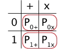
Figure 6.3: Original problem

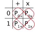
Figure 6.4: Derived problem

It may appear unrealistic to assume that the two STAR problems are essentially equal. Note however, that this is indeed the case in the example of the XOR function and two mutually unbiased bases (e.g. computational and Hadamard). The unitary here is just $U=\sigma_{z}\otimes\mathbb{I}^{\otimes n-1}$, as $\sigma_{z}$ acts as a bit-flip in the Hadamard basis, but leaves the computational basis invariant. We saw in the proof of Theorem 3.3.9 that such unitaries exist for any choice of two bases from the computational, Hadamard and K-basis. Indeed, for the XOR function on a string of length $n$ with $n$ even we saw that for STAR the optimal probability is $p=3/4$, whereas for PI-STAR we obtained $p=1$, as expected.

To generalize this approach, we need to consider more complicated inequalities. In general, there are many possibilities for such inequalities, and one should choose an inequality that reflects the equivalences of possible STAR problems: For example, for the XOR function the CHSH inequality is a good choice as we could identify $U=\sigma_{z}\otimes\mathbb{I}^{\otimes n-1}$ to give us an equivalence between the two problems. Of course, we would like to ensure that for one of Bob’s measurement settings he needs to solve the original STAR problem where Bob’s goal is to determine Alice’s measurement outcome. At the same time, we would like to minimize the number of possibly inequivalent additional STAR problems created in a similar proof, i.e. we would like to find an inequality where Bob has only a small number of measurement settings. As an example, we consider the following easy way to extend the CHSH inequality. Here, we assume that Alice has equally many measurement outcomes as she has measurement settings. In the language of PI-STAR that means we have wlog $A=\mathcal{Y}=S=\mathcal{B}$. We fix the number of Bob’s measurement settings to 2, but allow an arbitrarily large number of settings $|S|=|\mathcal{B}|$ for Alice. Wlog we use $T=\{0,1\}$ and $S=\{0,\ldots,|\mathcal{B}|-1\}$. We now define the predicate $V$ with the help of the function $\tau^{s}_{t}$ for $s\in S$ and $t\in T$. Let $\tau^{s}_{0}(y)=y$ for all $s\in S$ and let $\tau^{0}_{1}(y)=y$ and $\tau^{s}_{1}(y)=\sigma^{s}(y)$ for all $s\in\{1,\ldots,|\mathcal{B}|-1\}$, where $\sigma=(1,\ldots,|\mathcal{B}|-1)$ is the cyclic permutation. We now define the inequality as a non-local game with predicate $V(a,b|s,t)=1$ if and only if $b=\tau^{s}_{t}(a)$. Intuitively, this means that if Bob chooses setting $t=0$ he is required to solve the original STAR problem, where he tries to guess Alice’s measurement outcome. For the setting $t=1$ he has to solve the problem where the values of $y$ are shifted depending on the basis. Note that the CHSH inequality is a special case of this inequality. Recall from Section 6.2.3 that the optimal value of a classical game can always be attained by a deterministic strategy. Let $f_{A}:S\rightarrow\mathcal{Y}$ and $f_{B}:T\rightarrow\mathcal{Y}$ denote the functions implementing this strategy for Alice and Bob respectively. Looking at Eq. (6.3) we see that we can write

$$\omega_{c}(G)=\max\frac{1}{2|\mathcal{B}|}\sum_{t,s}[\tau^{s}_{t}(f_{A}(s))=f_{B}(t)],$$

where $[x=y]=1$ if and only if $x=y$. It is easy to see that for a uniform choice of Alice and Bob’s measurements, the best thing Bob can do is answer $f_{B}(t)=x$ for all $t$ where we choose any fixed $x\in\mathcal{Y}$ and let $x=f_{A}(s)$ for all $s\in S$, i.e. Alice and Bob agree on a particular outcome which will always be their answer regardless of their setting. For $t=0$ this means that Bob is always correct, and for $t=1$ he will be correct if Alice obtained $a=0$. We then have $\omega_{c}(G)=(|\mathcal{B}|+1)/(2|\mathcal{B}|)$. For the CHSH case, this gives us $\omega_{c}(G)=3/4$ as expected. It is now possible to make a similar statement then in Lemma 6.4.1 for a bigger PI-STAR problem.

The connection to Bell inequalities helped us understand the case where there exists a clear gap between the two problems. Here, post-measurement information was extremely helpful to us. However, as we saw in Chapter 3 there do exist cases where post-measurement information is entirely useless: we can do equally well without it, if we cannot store any quantum information. Interestingly, in the example of the XOR function on an odd number of input bits this happens exactly when the corresponding states correspond to a measurement that maximally violates CHSH. We have thus reached an extremal point of our problem. Is it possible to find conditions on a set of states which determine when post-measurement information is indeed useful?

6.5 Conclusion

As we saw, entanglement is an inherent aspect of quantum theory. We can experimentally violate Bell’s inequality, because we can indeed measure non-commuting observables. The existence of such violations is, next to uncertainty relations and locking, another consequence of the existence of non-commuting measurements within quantum theory. This illustrates their close link to uncertainty relations, locking and even post-measurement information we encountered in the preceding chapters. In essence, in all these tasks we are faced with exactly the same problem: what are the consequences of non-commuting measurements? And how can we find maximally “incompatible” measurements?

In the following chapters, we examine entanglement from a variety of viewpoints. In Chapter 7, we first consider Bell inequalities, and show how to find upper bounds on their violation in a quantum setting. Our approach allows us to find the optimal measurements for any bipartite correlation inequality with two-outcome measurements in a very easy manner. We then consider more general multipartite inequalities. Sadly, our method does not easily apply for more general inequalities. In fact, it is not even clear how large our optimization problem would have to be. We therefore consider a related problem in Chapter 8: Given a probability distribution over measurement outcomes, how large a state do we need to implement such a strategy? We prove a very weak lower bound on the dimension on the resulting state for a very restricted class of games. Finally, we consider the effects that entanglement has on classical protocols in Chapter 9. To this end we examine interactive proof systems where the two provers are allowed to share entanglement. Surprisingly, it turns out that two such provers can be simulated by just a single quantum prover.

Chapter 7 Finding optimal quantum strategies

In the previous chapter, we encountered the CHSH inequality and its generalizations in the guise of quantum games. Tsirelson has proven an upper bound on the CHSH inequality that can be achieved using a quantum strategy. But how can we prove upper bounds for more general inequalities? Or actually, how can we find the optimal measurement strategy? In this chapter, we answer these questions for a restricted class of inequalities by presenting a method that yields the optimal strategy for any two-player correlation inequality with $n$ measurement settings and two measurement outcomes, i.e. an XOR-game.

7.1 Introduction

Optimal strategies for generalized inequalities not only have applications in computer science with regard to interactive proof systems, but may also be important to ensure security in cryptographic protocols. From a physical perspective finding such bounds may also be helpful. As Braunstein and Caves [BC90b] have shown, it is interesting to consider inequalities based on many measurement settings, in particular, the chained CHSH inequality in Eq. 7.1 below: Here, the gap between the classical and the quantum bound is larger than for the original CHSH inequality with only two measurement settings. This can be helpful in real experiments that inevitably include noise, as this inequality leads to a larger gap achieved by the optimal classical and the quantum strategy, and may thus lead to a better test. However, determining bounds on the correlations that quantum theory allows remains a difficult problem [BM05]. All Tsirelson-type bounds are known for correlation inequalities with two measurement settings and two outcomes for both Alice and Bob [Tsi93]. Landau [Lan88] has taken a step towards finding Tsirelson-type bounds by considering when two-party correlations of two measurement settings for both Alice and Bob can be realized using quantum measurements. Filipp and Svozil [FS04] have considered the case of three measurement settings analytically and conducted numerical studies for a larger number of settings. Werner and Wolf [WW01a] also considered obtaining Tsirelson-type bounds for two-outcome measurements for multiple parties and studied the case of three and four settings explicitly. However, their method is hard to apply to general inequalities. Finally, Buhrman and Massar have shown a bound for a generalized CHSH inequality using three measurement settings with three outcomes each [BM05]. It is not known whether this bound can be attained.

Our approach is based on semidefinite programming in combination with Tsirelson’s seminal results [Tsi80, Tsi87, Tsi93] as outlined in Section 6.3.2. See Appendix A for a brief introduction to semidefinite programming. It is very easy to apply and gives tight bounds as we can find the optimal measurements explicitly. Let $X$ and $Y$ be Alice’s and Bob’s observables, and let $|\Psi\rangle$ be a state shared by Alice and Bob. The key benefit we derive from Tsirelson’s construction is that it saves us from the need to maximize over all states $|\Psi\rangle$ and observables. Instead, we can replace any terms of the form $\langle\Psi|X\otimes Y|\Psi\rangle$ with the inner product of two real unit vectors $x\cdot y$, and then maximize over all such vectors instead. Our method is thereby similar to methods used in computer science for the two-way partitioning problem [BV04] and the approximation algorithm for MAXCUT by Goemans and Williamson [GW95]. Semidefinite programming allows for an efficient way to approximate Tsirelson’s bounds for any CHSH-type inequalities numerically. However, it can also be used to prove Tsirelson type bounds analytically. As an illustration, we first give an alternative proof of Tsirelson’s original bound using semidefinite programming. We then prove a new Tsirelson-type bound for the following generalized CHSH inequality [Per93, BC90b]. Classically, it can be shown that

$$|\sum_{i=1}^{n}\langle X_{i}Y_{i}\rangle+\sum_{i=1}^{n-1}\langle X_{i+1}Y_{i}\rangle-\langle X_{1}Y_{n}\rangle|\leq 2n-2.$$ (7.1)

Here, we show that for quantum mechanics

$$|\sum_{i=1}^{n}\langle X_{i}Y_{i}\rangle+\sum_{i=1}^{n-1}\langle X_{i+1}Y_{i}\rangle-\langle X_{1}Y_{n}\rangle|\leq 2n\cos\left(\frac{\pi}{2n}\right),$$

where $\{X_{1},\ldots,X_{n}\}$ and $\{Y_{1},\ldots,Y_{n}\}$ are observables with eigenvalues $\pm 1$ employed by Alice and Bob respectively, corresponding to their $n$ possible measurement settings. It is well known that this bound can be achieved [Per93, BC90b] for a specific set of measurement settings if Alice and Bob share a singlet state. Here, we show that this bound is indeed optimal for any state $|\Psi\rangle$ and choice of measurement settings. This method generalizes to other CHSH inequalities, for example, the inequality considered by Gisin [Gis99].

7.2 A simple example: Tsirelson’s bound

To illustrate our approach we first give a detailed proof of Tsirelson’s bound using semidefinite programming. This proof is more complicated than Tsirelson’s original proof. However, it serves as a good introduction to the following section. Let $X_{1},X_{2}$ and $Y_{1},Y_{2}$ denote the observables with eigenvalues $\pm 1$ used by Alice and Bob respectively. Our goal is now to show an upper bound for

$$|\langle X_{1}Y_{1}\rangle+\langle X_{1}Y_{2}\rangle+\langle X_{2}Y_{1}\rangle-\langle X_{2}Y_{2}\rangle|.$$

From Theorem 6.3.6 we know that there exist real unit vectors $x_{s},y_{t}\in\mathbb{R}^{4}$ such that for all $s,t\in\{0,1\}$ $\langle X_{s}Y_{t}\rangle=x_{s}\cdot y_{t}$. In order to find Tsirelson’s bound, we thus want to solve the following problem: maximize $x_{1}\cdot y_{1}+x_{1}\cdot y_{2}+x_{2}\cdot y_{1}-x_{2}\cdot y_{2}$, subject to $\mbox{$\parallel{x_{1}}\parallel$}=\mbox{$\parallel{x_{2}}\parallel$}=\mbox{$\parallel{y_{1}}\parallel$}=\mbox{$\parallel{y_{2}}\parallel$}=1$. Note that we can drop the absolute value since any set of vectors maximizing the above equation, simultaneously leads to a set of vectors minimizing it by taking $-y_{1},-y_{2}$ instead. We now phrase this as a semidefinite program. Let $G=[g_{ij}]$ be the Gram matrix of the vectors $\{x_{1},x_{2},y_{1},y_{2}\}\subseteq\mathbb{R}^{4}$ with respect to the inner product:

$$G=\left(\begin{array}[]{cccc}x_{1}\cdot x_{1}&x_{1}\cdot x_{2}&x_{1}\cdot y_{1}&x_{1}\cdot y_{2}\\ x_{2}\cdot x_{1}&x_{2}\cdot x_{2}&x_{2}\cdot y_{1}&x_{2}\cdot y_{2}\\ y_{1}\cdot x_{1}&y_{1}\cdot x_{2}&y_{1}\cdot y_{2}&y_{1}\cdot y_{2}\\ y_{2}\cdot x_{1}&y_{2}\cdot x_{2}&y_{2}\cdot y_{1}&y_{2}\cdot y_{2}\end{array}\right).$$

$G$ can thus be written as $G=B^{T}B$ where the columns of $B$ are the vectors $\{x_{1},x_{2},y_{1},y_{2}\}$. By [HJ85, Theorem 7.2.11] we can write $G=B^{T}B$ if and only if $G$ is positive semidefinite. We thus impose the constraint that $G\geq 0$. To make sure that we obtain unit vectors, we add the constraint that all diagonal entries of $G$ must be equal to $1$. Define

$$W=\left(\begin{array}[]{cccc}0&0&1&1\\ 0&0&1&-1\\ 1&1&0&0\\ 1&-1&0&0\end{array}\right).$$

Note that the choice of order of the vectors in $B$ is not unique, however, a different order only leads to a different $W$ and does not change our argument. We can now rephrase our optimization problem as the following SDP:

maximize	$\frac{1}{2}\mbox{\rm Tr}(GW)$
subject to	$G\geq 0$ and $\forall i,g_{ii}=1$

We can then write for the Lagrangian

$$L(G,\lambda)=\frac{1}{2}\mbox{\rm Tr}(GW)-\mbox{\rm Tr}(\mbox{\rm diag}(\lambda)(G-I)),$$

where $\lambda=(\lambda_{1},\lambda_{2},\lambda_{3},\lambda_{4})$. The dual function is then

$$g(\lambda) = \sup_{G}\mbox{\rm Tr}\left(G\left(\frac{1}{2}W-\mbox{\rm diag}(\lambda)\right)\right)+\mbox{\rm Tr}(\mbox{\rm diag}(\lambda))$$

$$= \left\{\begin{array}[]{ll}\mbox{\rm Tr}(\mbox{\rm diag}(\lambda))&\mbox{if }\frac{1}{2}W-\mbox{\rm diag}(\lambda)\preceq 0\\[1.42262pt] \infty&\mbox{otherwise}\end{array}\right.$$

We then obtain the following dual formulation of the SDP

minimize	$\mbox{\rm Tr}(\mbox{\rm diag}(\lambda))$
subject to	$-\frac{1}{2}W+\mbox{\rm diag}(\lambda)\geq 0$

Let $p^{\prime}$ and $d^{\prime}$ denote optimal values for the primal and Lagrange dual problem respectively. From weak duality it follows that $d^{\prime}\geq p^{\prime}$. For our example, it is not difficult to see that this is indeed true as we show in Appendix A.

In order to prove Tsirelson’s bound, we now exhibit an optimal solution for both the primal and dual problem and then show that the value of the primal problem equals the value of the dual problem. The optimal solution is well known [Tsi80, Tsi87, Per93]. Alternatively, we could easily guess the optimal solution based on numerical optimization by a small program for Matlab and the package SeDuMi [SA] for semidefinite programming. Consider the following solution for the primal problem

$$G^{\prime}=\left(\begin{array}[]{cccc}1&0&\frac{1}{\sqrt{2}}&\frac{1}{\sqrt{2}}\\ 0&1&\frac{1}{\sqrt{2}}&-\frac{1}{\sqrt{2}}\\ \frac{1}{\sqrt{2}}&\frac{1}{\sqrt{2}}&1&0\\ \frac{1}{\sqrt{2}}&-\frac{1}{\sqrt{2}}&0&1\\ \end{array}\right),$$

which gives rise to the primal value $p^{\prime}=\frac{1}{2}\mbox{\rm Tr}(G^{\prime}W)=2\sqrt{2}$. Note that $G^{\prime}\geq 0$ since all its eigenvalues are non-negative [HJ85, Theorem 7.2.1], and all its diagonal entries are 1. Thus all constraints are satisfied. The lower left quadrant of $G^{\prime}$ is in fact the same as the well known correlation matrix for 2 observables [Tsi93, Equation 3.16]. Next, consider the following solution for the dual problem

$$\lambda^{\prime}=\frac{1}{\sqrt{2}}\left(1,1,1,1\right).$$

The dual value is then $d^{\prime}=\mbox{\rm Tr}(\mbox{\rm diag}(\lambda^{\prime}))=2\sqrt{2}$. Because $-W+\mbox{\rm diag}(\lambda^{\prime})\geq 0$, $\lambda^{\prime}$ satisfies the constraint. Since $p^{\prime}=d^{\prime}$, $G^{\prime}$ and $\lambda^{\prime}$ are in fact optimal solutions for the primal and dual respectively. We can thus conclude that

$$|\langle X_{1}Y_{1}\rangle+\langle X_{1}Y_{2}\rangle+\langle X_{2}Y_{1}\rangle-\langle X_{2}Y_{2}\rangle|\leq 2\sqrt{2},$$

which is Tsirelson’s bound [Tsi80]. By Theorem 6.3.6, this bound is achievable.

7.3 The generalized CHSH inequality

We now show how to obtain bounds for inequalities based on more than 2 observables for both Alice and Bob. In particular, we prove a bound for the chained CHSH inequality for the quantum case. It is well known [Per93] that it is possible to choose observables $X_{1},\ldots,X_{n}$ and $Y_{1},\ldots,Y_{n}$, and the maximally entangled state, such that

$$|\sum_{i=1}^{n}\langle X_{i}Y_{i}\rangle+\sum_{i=1}^{n-1}\langle X_{i+1}Y_{i}\rangle-\langle X_{1}Y_{n}\rangle|=2n\cos\left(\frac{\pi}{2n}\right).$$

We now show that this is optimal. Our proof is similar to the last section. However, it is more difficult to show feasibility for all $n$.

Theorem 7.3.1.

Let $\rho\in\mathcal{A}\otimes\mathcal{B}$ be an arbitrary state, where $\mathcal{A}$ and $\mathcal{B}$ denote the Hilbert spaces of Alice and Bob. Let $X_{1},\ldots,X_{n}$ and $Y_{1},\ldots,Y_{n}$ be observables with eigenvalues $\pm 1$ on $\mathcal{A}$ and $\mathcal{B}$ respectively. Then

$$|\sum_{i=1}^{n}\langle X_{i}Y_{i}\rangle+\sum_{i=1}^{n-1}\langle X_{i+1}Y_{i}\rangle-\langle X_{1}Y_{n}\rangle|\leq 2n\cos\left(\frac{\pi}{2n}\right),$$

Proof 7.3.2.

By Theorem 6.3.6, our goal is to find the maximum value for $x_{1}\cdot y_{1}+x_{2}\cdot y_{1}+x_{2}\cdot y_{2}+x_{3}\cdot y_{2}+\ldots+x_{n}\cdot y_{n}-x_{1}\cdot y_{n},$ for real unit vectors $x_{1},\ldots,x_{n},y_{1},\ldots,y_{n}\in\mathbb{R}^{2n}$. As above we can drop the absolute value. Let $G=[g_{ij}]$ be the Gram matrix of the vectors $\{x_{1},\ldots,x_{n},y_{1},\ldots,y_{n}\}\subseteq\mathbb{R}^{2n}$. As before, we can thus write $G=B^{T}B$, where the columns of $B$ are the vectors $\{x_{1},\ldots,x_{n},y_{1},\ldots,y_{n}\}$, if and only if $G\geq 0$. To ensure we obtain unit vectors, we again demand that all diagonal entries of $G$ equal $1$. Define $n\times n$ matrix $A$ and $2n\times 2n$ matrix $W$ by

$$A=\left(\begin{array}[]{ccccc}1&1&0&\ldots&0\\ 0&1&1&&\vdots\\ \vdots&&\ddots&\ddots&0\\ 0&&&1&1\\ -1&0&\ldots&0&1\\ \end{array}\right),\mbox{~{}}W=\left(\begin{array}[]{cc}0&A^{\dagger}\\ A&0\end{array}\right).$$

We can now phrase our maximization problem as the following SDP:

maximize	$\frac{1}{2}\mbox{\rm Tr}(GW)$
subject to	$G\geq 0$ and $\forall i,g_{ii}=1$

Analogous to the previous section, the dual SDP is then:

minimize	$\mbox{\rm Tr}(\mbox{\rm diag}(\lambda))$
subject to	$-\frac{1}{2}W+\mbox{\rm diag}(\lambda)\geq 0$

Let $p^{\prime}$ and $d^{\prime}$ denote optimal values for the primal and dual problem respectively. As before, $d^{\prime}\geq p^{\prime}$.

Primal

We now show that the vectors suggested in [Per93] are optimal. For $k\in[n]$, choose unit vectors $x_{k},y_{k}\in\mathbb{R}^{2n}$ to be of the form

$$x_{k} = (\cos(\phi_{k}),\sin(\phi_{k}),0,\ldots,0),$$

$$y_{k} = (\cos(\psi_{k}),\sin(\psi_{k}),0,\ldots,0),$$

where $\phi_{k}=\frac{\pi}{2n}(2k-2)$ and $\psi_{k}=\frac{\pi}{2n}(2k-1)$. The angle between $x_{k}$ and $y_{k}$ is given by $\psi_{k}-\phi_{k}=\frac{\pi}{2n}$ and thus $x_{k}\cdot y_{k}=\cos\left(\frac{\pi}{2n}\right)$. The angle between $x_{k+1}$ and $y_{k}$ is $\phi_{k+1}-\psi_{k}=\frac{\pi}{2n}$ and thus $x_{k+1}\cdot y_{k}=\cos\left(\frac{\pi}{2n}\right)$. Finally, the angle between $-x_{1}$ and $y_{n}$ is $\pi-\psi_{n}=\frac{\pi}{2n}$ and so $-x_{1}\cdot y_{n}=\cos\left(\frac{\pi}{2n}\right)$. The value of our primal problem is thus given by

$$p^{\prime}=\sum_{k=1}^{n}x_{k}\cdot y_{k}+\sum_{k=1}^{n-1}x_{k+1}\cdot y_{k}-x_{1}\cdot y_{n}=2n\cos\left(\frac{\pi}{2n}\right).$$

Let $G^{\prime}$ be the Gram matrix constructed from all vectors $x_{k},y_{k}$ as described earlier. Note that our constraints are satisfied: $\forall i:g_{ii}=1$ and $G^{\prime}\geq 0$, because $G^{\prime}$ is symmetric and of the form $G^{\prime}=B^{T}B$.

Dual

Now consider the $2n$-dimensional vector

$$\lambda^{\prime}=\cos\left(\frac{\pi}{2n}\right)\left(1,\ldots,1\right).$$

In order to show that this is a feasible solution to the dual problem, we have to prove that $-\frac{1}{2}W+\mbox{\rm diag}(\lambda^{\prime})\geq 0$ and thus the constraint is satisfied. To this end, we first show that

Claim 2.

The eigenvalues of $A$ are given by $\gamma_{s}=1+e^{i\pi(2s+1)/n}$ with $s=0,\ldots,n-1$.

Proof 7.3.3.

Note that if the lower left corner of $A$ were $1$, $A$ would be a circulant matrix [Gra71], i.e. each row of $A$ is constructed by taking the previous row and shifting it one place to the right. We can use ideas from circulant matrices to guess eigenvalues $\gamma_{s}$ with eigenvectors

$$u_{s}=(\rho_{s}^{n-1},\rho_{s}^{n-2},\rho_{s}^{n-3},\ldots,\rho_{s}^{1},\rho_{s}^{0}),$$

where $\rho_{s}=e^{-i\pi(2s+1)/n}$ and $s=0,\ldots,n-1$. By definition, $u=(u_{1},u_{2},\ldots,u_{n})$ is an eigenvector of $A$ with eigenvalue $\gamma$ if and only if $Au=\gamma u$. Here, $Au=\gamma u$ if and only if

$$(i) \forall j\in\{1,\ldots,n-1\}:u_{j}+u_{j+1}=\gamma u_{j},$$

$$(ii) -u_{1}+u_{n}=\gamma u_{n}.$$

Since for any $j\in\{1,\ldots,n-1\}$

$$u_{j}+u_{j+1} = \rho_{s}^{n-j}+\rho_{s}^{n-j-1}=$$

$$= e^{-i(n-j)\pi(2s+1)/n}(1+e^{i\pi(2s+1)/n})=$$

$$= \rho_{s}^{n-j}\gamma_{s}=\gamma_{s}u_{j},$$

(i) is satisfied. Furthermore (ii) is satisfied, since

$$-u_{1}+u_{n} = -\rho_{s}^{n-1}+\rho_{s}^{0}=$$

$$= -e^{-i\pi(2s+1)}e^{i\pi(2s+1)/n}+1=$$

$$= 1+e^{i\pi(2s+1)/n}=$$

$$= \gamma_{s}\rho_{s}^{0}=\gamma_{s}u_{n}.$$

Claim 3.

The largest eigenvalue of $W$ is given by $\gamma=2\cos\left(\frac{\pi}{2n}\right)$.

Proof 7.3.4.

By [HJ85, Theorem 7.3.7], the eigenvalues of $W$ are given by the singular values of $A$ and their negatives. It follows from Claim 2 that the singular values of $A$ are

$$\sigma_{s}=\sqrt{\gamma_{s}\gamma_{s}^{*}}=\sqrt{2+2\cos\left(\frac{\pi(2s+1)}{n}\right)}.$$

Considering the shape of the cosine function, it is easy to see that the largest singular value of $A$ is given by $\sqrt{2+2\cos(\pi/n)}=\sqrt{4\cos^{2}(\pi/(2n))}$, the largest eigenvalue of $W$ is $\sqrt{2+2\cos(\pi/n)}=2\cos(\pi/(2n))$.

Since $-\frac{1}{2}W$ and $\mbox{\rm diag}(\lambda^{\prime})$ are both Hermitian, Weyl’s theorem [HJ85, Theorem 4.3.1] implies that

$$\gamma_{min}\left(-\frac{1}{2}W+\mbox{\rm diag}(\lambda^{\prime})\right)\geq\gamma_{min}\left(-\frac{1}{2}W\right)+\gamma_{min}\left(\mbox{\rm diag}(\lambda^{\prime})\right),$$

where $\gamma_{min}(M)$ is the smallest eigenvalue of a matrix $M$. It then follows from the fact that $\mbox{\rm diag}(\lambda^{\prime})$ is diagonal and Claim 3 that

$$\gamma_{min}\left(-\frac{1}{2}W+\mbox{\rm diag}(\lambda^{\prime})\right)\geq-\frac{1}{2}\left(2\cos\left(\frac{\pi}{2n}\right)\right)+\cos\left(\frac{\pi}{2n}\right)=0.$$

Thus $-\frac{1}{2}W+\mbox{\rm diag}(\lambda^{\prime})\geq 0$ and $\lambda^{\prime}$ is a feasible solution to the dual problem. The value of the dual problem is then

$$d^{\prime}=\mbox{\rm Tr}(\mbox{\rm diag}(\lambda^{\prime}))=2n\cos\left(\frac{\pi}{2n}\right).$$

Because $p^{\prime}=d^{\prime}$, $G^{\prime}$ and $\lambda^{\prime}$ are optimal solutions for the primal and dual respectively, which completes our proof.

Note that for the primal problem we are effectively dealing with $2$-dimensional vectors, $x_{k},y_{k}$. As we saw in Section 6.3.2, it follows from Tsirelson’s construction [Tsi93] that in this case we just need a single EPR pair such that we can find observables that achieve this bound. In fact, these vectors just determine the measurement directions as given in [Per93].

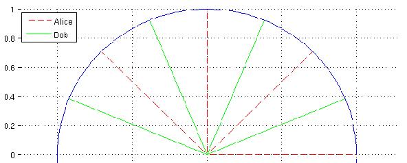
Figure 7.1: Optimal vectors for $n=4$ obtained numerically using Matlab.

7.4 General approach and its applications

7.4.1 General approach

Our approach can easily be generalized to other correlation inequalities. For another inequality, we merely use a different matrix $A$ in $W$. For example, for Gisin’s CHSH inequality [Gis99], $A$ is the matrix with 1’s in the upper left half and on the diagonal, and -1’s in the lower right part. Otherwise our approach stays exactly the same, and thus we do not consider this case here. Numerical results provided by our Matlab example code suggest that Gisin’s observables are optimal. Given the framework of semidefinite programming, the only difficulty in proving bounds for other inequalities is to determine the eigenvalues of the corresponding $A$, a simple matrix. All bounds found this way are tight, as we can always implement the resulting strategy using a maximally entangled state as shown in Section 6.3.2.

With respect to finding numerical bounds, we see that the optimal strategy can be found in time exponential in the number of measurement settings: The size of the vectors scales exponentially with the number of settings, however, we can fortunately find the optimal vectors in time polynomial in the length of the vectors using well-known algorithms for semidefinite programming [BV04].

7.4.2 Applications

In Chapter 9, we will see that the mere existence of such a semidefinite program has implications for the computational complexity of interactive proof systems with entanglement. Cleve, Høyer, Toner and Watrous [CHTW04a] have also remarked during their presentation at CCC’04 that Tsirelson’s constructions leads to an approach by semidefinite programming in the context of multiple interactive proof systems with entanglement, but never gave an explicit argument.

The above semidefinite program has also been used to prove results about compositions of quantum games, in particular, parallel repetitions of quantum XOR-games [CSUU07]. One particular type of composition studied by Cleve, Slofstra, Unger and Upadhyay [CSUU07] is the XOR-composition of non-local games. For example, an XOR-composition of a CHSH game is a new game where Alice and Bob each have $n$ inputs $x_{1},\ldots,x_{n}$ and $y_{1},\ldots,y_{n}$ with $x_{j},y_{j}\in\{0,1\}$ and must give answers $a$ and $b$ such that $a\oplus b=\bigoplus x_{j}\cdot y_{j}$. In terms of our semidefinite program, this is indeed easy to analyze. The matrix defining the game is now given by

$$A=\left(\begin{array}[]{cc}1&1\\ 1&-1\end{array}\right) W=\left(\begin{array}[]{cc}0&A^{\otimes n}\\ A^{\otimes n}&0\end{array}\right).$$

Note that the eigenvalues of $W$ are given by $\pm\sqrt{\gamma(A)\gamma(A)^{*}}$ where $\gamma(A)=\pm(\sqrt{2})^{n}$ is an eigenvalue of $A^{\otimes n}$. Consider the matrix $G=\mathbb{I}+W/(\sqrt{2})^{n}$. Clearly, $W/(\sqrt{2})^{n}$ has eigenvalues $\pm 1$ so we have $G\geq 0$. Thus $G$ is a valid solution to our primal problem, for which we obtain $p=\mbox{\rm Tr}(GW)/2=(2\sqrt{2})^{k}$. Consider $\lambda=(1,\ldots,1)((\sqrt{2})^{n}/2)$. Clearly, it is a valid solution to our dual problem as $-W/2+\mbox{\rm diag}(\lambda)\geq 0$, again using Weyl’s theorem. This gives for our dual problem $d=\mbox{\rm Tr}(\mbox{\rm diag}(\lambda))=(2\sqrt{2})^{n}=p$ and thus our primal solution is optimal. For more general problems, such a composition may be more complicated as the dual solution is not immediately related to the eigenvalues of $W$. Nevertheless, it can be readily evaluated using Schur’s complement trick [CSUU07]. By rewriting, one can then relate such compositions to the questions of parallel repetition: Given multiple runs of the game, does there exist a better quantum measurement than executing the optimal strategy of each round many times? It is very interesting that this is in fact not true for XOR-games [CSUU07]. However, there exist inequalities and specific quantum states for which collective measurements are better. Such examples can be found in the works of Peres [Per96] and Liang and Doherty [LD06]. Sadly, our approach fails here.

7.5 Conclusion

We have provided a simple method to obtain the optimal measurements for any bipartite correlation inequality, i.e. any two-player XOR game. Our method easily allows us to obtain bounds using numerical analysis, but also suits itself to construct analytical proofs as demonstrated by our examples. However, the above discussion immediately highlights the shortcomings of our approach. How can we find the optimal strategies for more generalized inequalities, where we have more than two players or a non-correlation inequality? Or more than two measurement outcomes? How can we find the optimal strategy for a fixed quantum state that is given to Alice and Bob? To address more than two measurement outcomes, we can rescale the observables such that they have eigenvalues in the interval $[-1,1]$. Indeed, examining Tsirelson’s proof, it is easy to see that we could achieve the same by demanding that the vectors have a length proportional to the number of settings. However, it is clear that the converse of Tsirelson’s theorem that allows us to construct measurement from the vectors can no longer hold. Indeed, any matrix $M=\sum_{j}m_{j}X_{j}$ that can be written as a sum of anti-commuting matrices $X_{1},\ldots,X_{n}$ with $X_{j}^{2}=\mathbb{I}$ and $\sum_{j}m_{j}^{2}=1$ must have eigenvalues $\pm 1$ itself since $M^{2}=\sum_{jk}m_{j}m_{k}X_{j}X_{k}=\left(\sum_{j}m_{j}^{2}\right)\mathbb{I}=\mathbb{I}$.

Since the completion of this work, exciting progress has been made to answer the above questions. Liang and Doherty [LD07] have shown how to obtain lower and upper bounds on the optimal strategy achievable using a fixed quantum state using semidefinite programming relaxations. Kempe, Kobayashi, Matsumoto, Toner and Vidick [KKM⁺07] have since shown that there exist three-player games for which the optimal quantum strategy cannot be computed using a semidefinite program that is exponential in the number of measurement settings unless P=NP. Finally, Navascués, Pironio and Acín [NPA07] have shown how to obtain bounds for general two-party inequalities with more measurement outcomes using semidefinite programming, inspired by Landau [Lan88]. Their beautiful approach used successive hierarchies of semidefinite programs to obtain better and better bounds. In their approach, they consider whether a given distribution over outcomes can be obtained using a quantum strategy. Sadly, it does not give a general method to construct actual measurements and thus show that an obtained bound is tight. A similar result obtained using an approach that is essentially dual to [NPA07] has been obtained in [DLTW08], which also proves a convergence result for such a hierarchy.

One of the difficulties we face when trying to find tight bounds for more general inequalities is to determine how large our optimization problem has to be. But even if we are given some distribution over possible outcomes, how can we decide how large our system has to be in order to implement a quantum strategy? In general, this is a tricky problem which we will consider in the next chapter.

Chapter 8 Bounding entanglement in NL-games

In the previous chapter, we provided a simple method to determine the optimal quantum strategy for two-outcome XOR games. However, when trying to find the optimal strategies for more general games, we are faced with a fundamental issue: How large do we have to choose our state and measurements such that we can achieve the optimal quantum value?

8.1 Introduction

Determining an upper bound and the amount of entanglement we need, given the description of the game alone, turns out to be a tricky problem in the general case. Hence, we address an intermediate problem: Given the description of a non-local game and associated probabilities, how large a state do Alice and Bob need to implement such a strategy? Navascués, Pironio and Acín [NPA07] and also [DLTW08] have shown how to obtain upper bounds for the violation of more general quantum games using multiple hierarchies of semidefinite programs. However, their method does not provide us with an explicit strategy, and it remains unclear how many levels of the hierarchy we need to consider in order to obtain a tight bound. Yet, from their method we can obtain a probability distribution over measurement outcomes. Using our approach, we can then determine an extremely weak lower bound on the dimension of the quantum state we would need in order to implement a corresponding quantum strategy.

The idea behind our approach is to transform a non-local game into a random access code. A random access code is an encoding of a string into a quantum state such that we can retrieve at least one entry of our choice from this string with some probability. Intuitively, Alice’s measurements will create an encoding. Bob’s choice of measurement then determines which bit of this “encoding” he wants to retrieve. We prove a general lower bound for any independent one-to-one non-local game among $n$ players, where a one-to-one non-local game is a game where for each possible measurement setting there exists exactly one correct measurement outcome. In particular, we show that in any one-to-one non-local game where player $P_{j}$ obtains the correct outcome $a\in A_{j}$ for any measurement setting $s\in S_{j}$ with probability $p$ the dimension $d$ of player $P_{j}$’s state obeys

$$d\geq 2^{(\log|A_{j}|-H(p)-(1-p)\log(|A_{j}|-1))|S_{j}|}.$$

Even though our bound is very weak, and the class of games very restricted, we are hopeful that our approach may lead to stronger results in the future. Finally, we discuss how we could obtain upper bounds from the description of the non-local game alone without resorting to probability distributions.

8.2 Preliminaries

Before we can prove our lower bound, we first introduce the notion of a random access code. For our purposes, we need to generalize the existing results on random access codes. We use $M(\rho)$ to denote the random variable corresponding to the outcome of a measurement $M$ on a state $\rho$. We also use $A^{n}$ to denote an $n$-element string where each element is chosen from an alphabet $A$. We will also use the notation $\vec{s}_{-j}$ to denote the string $\vec{s}=(s_{1},\ldots,s_{n})$ without the element $s_{j}$.

8.2.1 Random access codes

A quantum $(n,m,p)$-random access code (RAC) [ANTV99, Nay99] over a binary alphabet is an encoding of an $n$-bit string $x$ into an $m$-qubit state $\rho_{x}$ such that for any $i\in[n]$ we can retrieve $x_{i}$ from $\rho_{x}$ with probability $p$. Note that we are only interested in retrieving a single bit of the original string $x$ from $\rho_{x}$. In general, it is unlikely we will be able to retrieve more than a single bit. For such codes the following lower bound has been shown [Nay99, Theorem 2.3], where it is assumed that the original strings $x$ are chosen uniformly at random:

Theorem 8.2.1 (Nayak).

Any $(n,m,p)$-random access code has $m\geq(1-H(p))n$.

In the following, we make use of a generalization of random access codes to larger alphabets. We also need two additional generalizations: First, we also want to obtain a bound on such a RAC encoding if the string $x$ is chosen from a slightly more general, possibly non-uniform, distribution. Let $P_{X_{t}}$ be a probability distribution over $\Sigma$ and let $P_{X}=P_{X_{1}}\times\ldots\times P_{X_{n}}$ be a probability distribution over $\Sigma^{n}$. That is, a particular string $x$ is chosen with probability $P_{X}(x)=\Pi_{t=1}^{n}P_{X_{t}}(x_{t})$. Note that we assume that the individual entries of $x$ are chosen independently.

Second, we allow for unbalanced random access codes, where each entry of the string $x$ may have a different probability of being decoded correctly. We define

Definition 8.2.2.

An $(n,m,(p_{1},\ldots,p_{n}))_{|\Sigma|}$-unbalanced random access code (URAC) over a finite alphabet $\Sigma$ is an encoding of an $n$-element string $x\in\Sigma^{n}$ into an $m$-qubit state $\rho_{x}$ such that for any $t\in[n]$, there exists a measurement $M_{t}$ with outcomes $\Sigma$ such that for all $x\in\Sigma^{n}$ we have $\Pr[M_{t}(\rho_{x})=x_{t}]\geq p_{t}$.

Fortunately, it is straightforward to extend the analysis of Nayak [Nay99] to this setting. We extend the proof by Nayak as opposed to other known proofs of this lower bound in order to deal with unbalanced random access codes more easily.

Lemma 8.2.3.

Let $P_{X}=P_{X_{1}}\times\ldots\times P_{X_{n}}$ be a probability distribution over $\Sigma^{n}$. Then any $(n,m,(p_{1},\ldots,p_{n}))_{|\Sigma|}$-unbalanced random access code has

$$m\geq\sum_{t=1}^{n}H(X_{t})-H(p_{t})-(1-p_{t})\log(|\Sigma|-1)$$

where $X_{t}$ is a random variable chosen from $\Sigma$ according to the probability distribution $P_{X_{t}}$.

Proof 8.2.4.

The proof follows along the same lines as Lemma 4.1 and Claim 4.6 of [Nay99]. We state the adaption for clarity:

We first consider decoding a single element. Let $\sigma_{a}$ with $a\in\Sigma$ be density matrices, and let $P$ be a probability distribution over $\Sigma$. Define $\sigma=\sum_{a\in\Sigma}P(a)\sigma_{a}$. Let $M$ be a measurement with outcomes $\Sigma$ that given any state $\sigma_{a}$ gives the correct outcome $a$ with average probability $p$. Let $X$ be a random variable over $\Sigma$ chosen according to probability distribution $P$, and let $Z$ be a random variable over $\Sigma$ corresponding to the outcome of the measurement. It now follows from Fano’s inequality (see for example [Hay06, Theorem 2.2]) that $\mathcal{I}(X,Z)=H(X)-H(X|Z)\geq H(X)-H(p)-(1-p)\log(|\Sigma|-1)$. Using Holevo’s bound, we then have $S(\sigma)\geq\sum_{a\in\Sigma}P(a)S(\sigma_{a})+H(X)-H(p)-(1-p)\log(|\Sigma|-1)$.

We now consider an entire string $x$ encoded as a state $\rho_{x}$. Consider $k$ with $n\geq k\geq 0$ and define $\rho_{y}=\sum_{z\in\Sigma^{n-k}}q_{z}\rho_{zy}$ with $q_{z}=\Pi_{j=n-k}^{n}P_{X_{j}}(z_{j})$ where we used indices $z=z_{n},\ldots,z_{n-k}$ and $P_{X_{j}}$ to denote the probability distribution over $\Sigma$ according to which the $j$-th entry was encoded. We now claim that $S(\rho_{y})\geq\sum_{a\in\Sigma}P_{X_{n-k}}(a)S(\rho_{ay})+H(X_{n-k})-H(p_{n-k})-(1-p_{n-k})\log(|\Sigma|-1)$. The proof follows by downward induction over $k$: Consider $n=k$, clearly $S(\rho_{y})\geq 0$ and the claim is valid. Now suppose our claim holds for $k+1$. Note that we have $\rho_{y}=\sum_{a\in\Sigma}P_{X_{n-k}}(a)\rho_{ay}$. Note that strings encoded by the density matrices $\rho_{ay}$ only differ by one element $a\in\Sigma$. We can therefore distinguish them with probability $p_{n-k}$. From the above discussion we have that $S(\rho_{y})\geq\sum_{a\in\Sigma}P_{X_{n-k}}(a)S(\rho_{ay})+H(X_{n-k})-H(p_{n-k})-(1-p_{n-k})\log(|\Sigma|-1)$.

Using the inductive hypothesis, letting $y$ be the empty string and using the fact that $S(\rho)\leq\log d=m$ then completes the proof.

8.2.2 Non-local games and state discrimination

For our purpose, we need to think of non-local games as a special form of state discrimination. When each subset of players performs a measurement on their part of the state, they effectively prepare a certain state on the system of the remaining players. Let $\chi_{\vec{a}_{-j}}^{\vec{s}_{-j}}$ denote the state of Player $P_{j}$ if the remaining players chose measurement settings $\vec{s}_{-j}$ and obtained outcomes $\vec{a}_{-j}$. Note that the probability that player $P_{j}$ holds $\chi_{\vec{a}_{-j}}^{\vec{s}_{-j}}$ is $\Pr[\vec{a}_{-j},\vec{s}_{-j}]=\Pr[\vec{a}_{-j}|\vec{s}_{-j}]\Pi_{\ell=1,\ell\neq j}^{N}\pi_{\ell}(s_{\ell})$. Define the state

$$\zeta^{s_{j}}_{a_{j}}=\frac{1}{q^{s_{j}}_{a_{j}}}\left(\sum_{\vec{s}_{-j}}\sum_{\vec{a}_{-j}}V(\vec{a}|\vec{s})\Pr[\vec{a}_{-j}|\vec{s}_{-j}]\chi_{\vec{a}_{-j}}^{\vec{s}_{-j}}\right)$$

where $q^{s_{j}}_{a_{j}}=\sum_{\vec{s}_{-j}}\sum_{\vec{a}_{-j}}V(\vec{a}|\vec{s})\Pr[\vec{a}_{-j}|\vec{s}_{-j}]$ to ensure normalization. We call a game independent, if the sets of probabilities $\{q^{u}_{a_{j}}\mid a_{j}\in A_{j}\}$ and $\{q^{v}_{a_{k}}\mid a_{k}\in A_{j}\}$ are uncorrelated for all measurement settings $u,v\in S_{j}$ with $u\neq v$. Note that $q^{s_{j}}_{a_{j}}$ is the probability that player $P_{j}$ holds state $\zeta^{s_{j}}_{a_{j}}$, and that $\sum_{a_{j}\in A_{j}}q^{s_{j}}_{a_{j}}=1$ since the game is one-to-one. If player $P_{j}$ now chooses measurement setting $s_{j}$ he is effectively trying to solve a state discrimination problem, given the ensemble $\{q^{s_{j}}_{a_{j}},\zeta^{s_{j}}_{a_{j}}|a_{j}\in A_{j}\}$.

Note that we already encountered this viewpoint in Chapter 6.4. Consider the simple case of the CHSH game. Here, Alice (Player 1) and Bob (Player 2) had to give answers $a_{1}$ and $a_{2}$ for settings $s_{1}$ and $s_{2}$ such that $s_{1}\cdot s_{2}=a_{1}\oplus a_{2}$. Let $\zeta_{a_{1}}^{s_{1}}$ denote Bob’s state if Alice chose measurement setting $s_{1}$ and obtained outcome $a_{1}$. If Bob chooses setting $s_{2}=0$, he has to solve the state discrimination problem described by Figure 6.4: he must answer $a_{2}=a_{1}$, and hence his goal is to learn $a_{1}$. That is, he must solve the state discrimination problem given by $\rho_{0}=(\zeta_{0}^{0}+\zeta_{0}^{1})/2$ and $\rho_{1}=(\zeta_{1}^{0}+\zeta_{1}^{1})/2$. For $s_{2}=1$, he has to solve the problem given by Figure 6.4: For $s_{1}=0$, he must answer $a_{2}=a_{1}$, but for $s_{1}=1$ he must answer $a_{2}\neq a_{1}$. Hence, he must solve the state discrimination problem given by $\tilde{\rho}_{0}=(\zeta_{0}^{0}+\zeta_{1}^{1})/2$ and $\tilde{\rho}_{1}=(\zeta_{1}^{0}+\zeta_{0}^{1})/2$.

8.3 A lower bound

We now show how to obtain a random access encoding from a one-to-one non-local game. This enables us to find a lower bound on the dimension of the quantum state necessary for any player $P_{j}$ to implement particular non-local strategies. Recall that we are trying to give a bound given all parameters of the game. In particular, we are given the probabilities $\Pr[\vec{a}_{-j}|\vec{s}_{-j}]$ that the remaining players obtain outcomes $\vec{a}_{-j}$ for their measurement settings $\vec{s}_{-j}$, as well as the value of the game. Note that we do not need to know an actual state and measurement strategy for the players. We just want to give a lower bound for a chosen set of parameters, whether these can be obtained or not.

Theorem 8.3.1.

Any one-to-one independent non-local game where player $P_{j}$ obtains the correct outcome $a_{j}\in A_{j}$ for measurement setting $s_{j}\in S_{j}$ with probability $p_{s_{j}}$ for all $\vec{s}_{-j}\in S_{1}\times\ldots\times S_{j-1}\times S_{j+1}\times\ldots\times S_{N}$ and $\vec{a}_{-j}\in A_{1}\times\ldots\times A_{j-1}\times A_{j+1}\times\ldots\times A_{N}$ is a $(|S_{j}|,m,(p_{1},\ldots,p_{|S_{j}|}))_{|A_{j}|}$-unbalanced random access code.

Proof 8.3.2.

To encode a string, the other players choose measurement settings $\vec{s}_{-j}$ and measure their part of the state as in the non-local game to obtain outcomes $\vec{a}_{-j}$. Note that the string is chosen randomly by the measurement. Since our game was one-to-one we can define a function

$$g(\vec{s}_{-j},\vec{a}_{-j})=f_{1}(\vec{s}_{-j},\vec{a}_{-j}),\ldots,f_{|S_{j}|}(\vec{s}_{-j},\vec{a}_{-j}).$$

Let $x=g(\vec{s}_{-j},\vec{a}_{-j})$ be the encoded string and note that $\rho_{x}=\chi_{\vec{a}_{-j}}^{\vec{s}_{-j}}$. We have $P_{X_{t}}(c)=q^{s_{j}}_{c}$, since our game is one-to-one. Since our game is independent, we have that $P_{X}$ is a product distribution. To retrieve the $t$-th entry of $x$, player $P_{j}$ then has to distinguish $\zeta_{a_{j}}^{s_{j}}$ as in the non-local game which he can do with probability $p_{s_{j}}$ by assumption.

Now that we can obtain a random access code from a non-local game, we can easily give a lower bound on the dimension of the state from a lower bound of the size of the random access code. It follows immediately from Theorem 8.3.1 and Lemma 8.2.3 that

Corollary 8.3.3.

In any one-to-one independent non-local game where player $P_{j}$ obtains the correct outcome $a\in A_{j}$ for measurement setting $s\in S_{j}$ with probability $p_{s}$ for all measurement settings $\vec{s}_{-j}\in S_{1}\times\ldots\times S_{j-1}\times S_{j+1}\times\ldots\times S_{N}$ and outcomes $\vec{a}_{-j}\in A_{1}\times\ldots\times A_{j-1}\times A_{j+1}\times\ldots\times A_{N}$ of the other players, the dimension $d$ of player $P_{j}$’s state obeys

$$d\geq 2^{\sum_{t=1}^{|S_{j}|}H(X_{t})-H(p_{t})-(1-p_{t})\log(|A_{j}|-1)},$$

where $X_{t}$ is a random variable chosen from $A_{j}$ where $\Pr[X_{t}=a]=q^{t}_{a}$.

For almost all known games, we can obtain a simplified bound as each player will choose a measurement setting uniformly at random. Likewise, in most cases we can assume that the probability that the players obtain certain outcomes is also uniform. Indeed, if we do not know a particular measurement strategy for a given game, we can find a bound if we assume that the distribution over the outcomes given the choice of measurement settings is uniform. In this case, we also assume that the probability of giving the correct answer is the same for each possible choice of measurement settings and is equal to the value of the game. We then obtain

Corollary 8.3.4.

In any one-to-one independent non-local game where player $P_{j}$ obtains the correct outcome $a\in A_{j}$ for any measurement setting $s\in S_{j}$ with probability $p$ where $q^{t}_{a}=1/|A_{j}|$ for all $t\in S_{j}$ and measurement settings $\vec{s}_{-j}\in S_{1}\times\ldots\times S_{j-1}\times S_{j+1}\times\ldots\times S_{N}$ and outcomes $\vec{a}_{-j}\in A_{1}\times\ldots\times A_{j-1}\times A_{j+1}\times\ldots\times A_{N}$ of the other players, the dimension $d$ of player $P_{j}$’s state obeys

$$d\geq 2^{(\log(|A_{j}|)-H(p)-(1-p)\log(|A_{j}|-1))|S_{j}|}.$$

Note that if we are willing to assume that the optimal value of the game is achieved when the players share a maximally entangled state, we can improve this bound to $d\geq\max_{j}2^{(\log(|A_{j}|)-H(p)-(1-p)\log(|A_{j}|-1))|S_{j}|}$.

Let’s look at a small example which illustrates the proof. Consider the CHSH inequality. Here, we have only two players, Alice (Player 1) and Bob (Player 2). Bob’s goal is to obtain an outcome $a_{2}$ such that $s_{1}\cdot s_{1}=a_{1}+a_{2}\mod 2$. This means we define the function $g(s_{1},a_{1})=x$ as $g(0,0)=0,0$, $g(1,0)=1,1$, $g(0,1)=1,0$ and $g(1,1)=0,1$. For the lower bound we do not need to consider a specific encoding, however, for the well-known CHSH state and measurements we would have an encoding of $\rho_{00}=|0\rangle\langle 0|$, $\rho_{01}=|-\rangle\langle-|$, $\rho_{10}=|+\rangle\langle+|$, and $\rho_{11}=|1\rangle\langle 1|$ and $q_{x_{1}}^{1}=q_{x_{2}}^{2}=1/2$ for all $x_{1},x_{2}\in\{0,1\}$. How many qubits does Bob need to use if he wants to give the correct answers with probability $p=1/2+1/(2\sqrt{2})$? Since everything is uniform we obtain $\log d\geq(1-H(p))2\approx 0.8$, i.e., Bob needs to keep at least one qubit.

Our bound contains a tradeoff between the probability $p$ of giving the correct answer, the number of measurement settings, and the number of possible outcomes. Clearly, our bound will only be good, if the number of measurement settings is large. It is also clear that it performs badly as $p$ approaches $1/2$ and $|A_{j}|$ is large, and thus for most cases our bound will be very unsatisfactory. The following figures illustrate the tradeoff between the different parameters of Corollary 8.3.4.

Figure 8.1: Tradeoff for $p=0.6$.

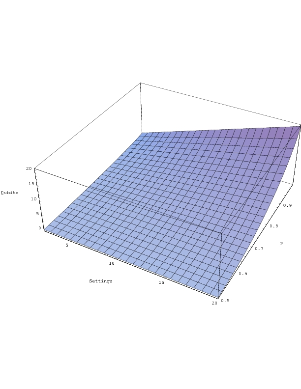
Figure 8.2: Tradeoff for 2 outcomes.

8.4 Upper bounds

Ideally, we would find an upper bound on the amount of entanglement we need purely from the description of the game alone. Clearly, Tsirelson’s construction from Chapter 6.3.2 tells us that for any XOR game the local dimension of Alice’s and Bob’s system is $d\leq 2^{N/2}$, where $N$ is the number of measurement settings. Similarly to XOR games, we can consider mod $k$-games. Here, Alice and Bob have to give answers $a_{1}$, $a_{2}$ given questions $s_{1}$, $s_{1}$ such that $f(s_{1},s_{2})=a_{1}+a_{2}\mod k$ for some function $f:S_{1}\times S_{2}\rightarrow\{0,\ldots,k-1\}$. One may hope that for mod $k$-games, similarly than for XOR-games, the following holds:

Conjecture 8.4.1.

For any mod $k$-game, the dimension of Alice’s and Bob’s systems obeys $d\leq k^{N/2}$, where $N$ is the number of measurement settings for Alice and Bob.

An alternative approach to bounding the dimension would be to consider how far we can reduce the size of an existing state and observables using Lemma 6.3.1. Suppose that Alice has only two measurement settings $X_{0}=X_{0}^{0}-X_{0}^{1}$ and $X_{1}=X_{1}^{0}-X_{1}^{1}$ with $X_{0}^{0}+X_{0}^{1}=\mathbb{I}$ and $X_{1}^{0}+X_{1}^{1}=\mathbb{I}$. We know from Lemma 3.5.3 that there exist projectors $\Pi_{j}$ such that we can decompose $X_{s}$ as $X_{s}=\sum_{j}\Pi_{j}X_{s}^{a}\Pi_{j}$ for $s,b\in{0,1}$, where $\mbox{rank}(\Pi_{j})\leq 2$. Hence, we can immediately conclude from Lemma 6.3.1 that if Alice only measures two possible observables with two outcomes each, the dimension of her state does not need to exceed $d=2$. This has previously been proved by Masanes [Mas06]. Could we prove something similar for three measurement settings? Sadly, Theorem 3.5.12 tells us that this is not possible! There do exist three measurements for which no such decomposition exists. It is not hard to see that the question of how large Alice’s entangled state has to be given a specific set of measurement operators is essentially equivalent to the question of how many qubits we need to store in the problem of post-measurement information to achieve perfect success. In both settings we are interested in reducing the dimension by finding a way to block-diagonalize the matrices.

8.5 Conclusion

Bounding the amount of entanglement that we need to implement the optimal strategy in non-local games remains a tricky problem. We have given a simple lower bound on the amount of entanglement necessary for an extremely restricted class of games. The CHSH game forms an instance of such a game. Even though our bound is very weak, and the class of games quite restricted, we are hopeful that our approach may lead to stronger statements in the future. We also showed how our earlier considerations and Tsirelson’s construction led to an upper bound for the specific case of XOR-games. Sadly, better bounds still elude us so far.

Chapter 9 Interactive Proof Systems

As we saw in the past chapters, two spatially separated parties, Alice and Bob, can use entanglement to obtain correlations that are impossible to achieve classically, without any additional communication. However, there do exist classical systems whose strength, or security, indeed depends crucially on the fact that specific parties cannot communicate during the course of the protocol. How are such systems affected by the presence of entanglement? Can Alice and Bob use their shared entanglement to gain a significant advantage? Here, we study interactive proof systems which are a specific case of such a classical system. Surprisingly, it turns out that the space-like separation is lost alltogether and we can simulate two classical parties with just a single quantum one.

9.1 Introduction

9.1.1 Classical interactive proof systems

Before getting to the heart of the matter, we first need to take a closer look at interactive proof systems. Classical interactive proof systems have received considerable attention [BFL91, BOGKW88, CCL90, Fei91, LS91, FL92] since their introduction by Babai [Bab85] and Goldwasser, Micali and Rackoff [GMR89] in 1985. An interactive proof system takes the form of a protocol of one or more rounds between two parties, a verifier and a prover. Whereas the prover is computationally unbounded, the verifier is limited to probabilistic polynomial time. Both the prover and the verifier have access to a common input string $x$. The goal of the prover is to convince the verifier that $x$ belongs to a pre-specified language $L$. The verifier’s aim, on the other hand, is to determine whether the prover’s claim is indeed valid. In each round, the verifier sends a polynomial (in $x$) size query to the prover, who returns a polynomial size answer. At the end of the protocol, the verifier decides to accept, and conclude $x\in L$, or reject based on the messages exchanged and his own private randomness. A language has an interactive proof if there exists a verifier $V$ and a prover $P$ such that: If $x\in L$, the prover can always convince $V$ to accept. If $x\notin L$, no strategy of the prover can convince $V$ to accept with non-negligible probability. IP denotes the class of languages having an interactive proof system. Watrous [Wat99] first considered the notion of quantum interactive proof systems. Here, the prover has unbounded quantum computational power whereas the verifier is restricted to quantum polynomial time. In addition, the two parties can now exchange quantum messages. QIP is the class of languages having a quantum interactive proof system. Classically, it is known that $\mbox{IP}=\mbox{PSPACE}$ [Sha92, She92], where PSPACE is the class of languages decidable using only polynomial space. For the quantum case, it has been shown that $\mbox{PSPACE}\subseteq\mbox{QIP}\subseteq\mbox{EXP}$ [Wat99, KW00]. If, in addition, the verifier is given polynomial size quantum advice, the resulting class $\mbox{QIP}/\mbox{qpoly}$ contains all languages [Raz05]. Let $\mbox{QIP}(k)$ denote the class where the prover and verifier are restricted to exchanging $k$ messages. It is known that $\mbox{QIP}=\mbox{QIP}(3)$ [KW00] and $\mbox{QIP}(1)\subseteq\mbox{PP}$ [Vya03, MW05], where PP is the class of all problems solvable by a probabilistic machine in polynomial time. We refer to [MW05] for an overview of the extensive work done on $\mbox{QIP}(1)$, also known as QMA. Very little is known about $\mbox{QIP}(2)$ and its relation to either PP or PSPACE.

In multiple-prover interactive proof systems the verifier can interact with multiple, computationally unbounded provers. Before the protocol starts, the provers are allowed to agree on a joint strategy, however they can no longer communicate during the execution of the protocol. Let MIP denote the class of languages having a multiple-prover interactive proof system. Here, we are especially interested in two-prover interactive proof systems as introduced by Ben-Or, Goldwasser, Kilian and Widgerson [BOGKW88]. Babai, Fortnow and Lund [BFL91], and Feige and Lovász [FL92] have shown that a language is in NEXP if and only if it has a two-prover one-round proof system, i.e., MIP[2] = NEXP. Feige and Lovász have also shown that a system using more than two-provers is thus no more powerful than a system with only two provers, i.e., MIP[2] = MIP. Let $\oplus\mbox{MIP}[2]$ denote the restricted class where the verifier’s output is a function of the XOR of two binary answers. Even for such a system $\oplus\mbox{MIP}[2]=\mbox{NEXP}$, for certain soundness and completeness parameters [CHTW04a]. Classical multiple-prover interactive proof systems are thus more powerful than classical proof systems based on a single prover, assuming $\mbox{PSPACE}\neq\mbox{NEXP}$.

9.1.2 Quantum multi-prover interactive proof systems

Given the advent of quantum computing, one can also consider quantum interactive proof systems with multiple provers. These can be grouped into two categories: First, one can consider provers and a verifier that are quantum themselves and can exchange quantum messages. Kobayashi and Matsumoto have considered such quantum multiple-prover interactive proof systems which form an extension of quantum single prover interactive proof systems as described above. Let QMIP denote the resulting class. In particular, they showed that $\mbox{QMIP}=\mbox{NEXP}$ if the provers do not share quantum entanglement [KM03]. If the provers share at most polynomially many entangled qubits the resulting class is contained in NEXP [KM03].

Secondly, one can consider proof systems where all communication remains classical, but the provers can share any entangled state as part of their strategy on which they are allowed to perform arbitrary measurements. Cleve, Høyer, Toner and Watrous [CHTW04a] have raised the question whether a classical two-prover system is weakened in such a setting. We write $\mbox{MIP}^{*}$ if the provers share entanglement. The authors provide a number of examples which demonstrate that the soundness condition of a classical proof system can be compromised, i.e. the interactive proof system is weakened, when entanglement is used. In their paper, it is proved that $\oplus\mbox{MIP}^{*}[2]\subseteq\mbox{NEXP}$. Later, the same authors also showed that $\oplus\mbox{MIP}^{*}[2]\subseteq\mbox{EXP}$ using semidefinite programming [CHTW04b]. Entanglement thus clearly weakens an interactive proof system, assuming $\mbox{EXP}\neq\mbox{NEXP}$.

Intuitively, entanglement allows the provers to coordinate their answers, even though they cannot use it to communicate. By measuring the shared entangled state the provers can generate correlations which they can use to deceive the verifier. Tsirelson [Tsi80, Tsi87] has shown that even quantum mechanics limits the strength of such correlations, as we saw in Chapter 6. Recall that Popescu and Roehrlich [PR94, PR96, PR97] have raised the question why nature imposes such limits. To this end, they constructed a toy-theory based on non-local boxes [PR94, vD00], which are hypothetical “machines” generating correlations stronger than possible in nature. In their full generalization, non-local boxes can give rise to any type of correlation as long as they cannot be used to signal. Preda [Pre05] showed that sharing non-local boxes allows two provers to coordinate their answers perfectly and obtained $\oplus\mbox{MIP}_{\mbox{\tiny{NL}}}=\mbox{PSPACE}$, where we write $\oplus\mbox{MIP}_{\mbox{\tiny{NL}}}$ to indicate that the two provers share non-local boxes.

Kitaev and Watrous [KW00] mention that it is unlikely that a single-prover quantum interactive proof system can simulate multiple classical provers, because then from $\mbox{QIP}\subseteq\mbox{EXP}$ and $\mbox{MIP}=\mbox{NEXP}$ it follows that $\mbox{EXP}=\mbox{NEXP}$.

Surprisingly, it turns out that when the provers are allowed to share entanglement it can be possible to simulate two such classical provers by one quantum prover. This indicates that entanglement among provers truly leads to a weaker proof system. In particular, we show that a two-prover one-round interactive proof system where the verifier computes the XOR of two binary answers and the provers are allowed to share an arbitrary entangled state, can be simulated by a single quantum interactive proof system with two messages: $\oplus\mbox{MIP}^{*}[2]\subseteq\mbox{QIP(2)}$. Since very little is known about $\mbox{QIP}(2)$ so far [KW00], we hope that our result may help shed some light on its relation to PP or PSPACE. Our result also leads to a proof that $\oplus\mbox{MIP}^{*}[2]\subseteq\mbox{EXP}$.

9.2 Proof systems and non-local games

9.2.1 Non-local games

For our proof, it is necessary to link interactive proof systems to non-local games, as we described in Chapter 6.2.3. Since we consider only two parties, we omit unnecessary indices and use separate letters to refer to the sets of possible questions and answers. We briefly recap our setup, summarized in Figure 9.1: Let $S$, $T$, $A$ and $B$ be finite sets, and $\pi$ a probability distribution on $S\times T$. Let $V$ be a predicate on $S\times T\times A\times B$. Then $G=G(V,\pi)$ is the following two-person cooperative game: A pair of questions $(s,t)\in S\times T$ is chosen at random according to the probability distribution $\pi$. Then $s$ is sent to player 1, henceforth called Alice, and $t$ to player 2, which we call Bob. Upon receiving $s$, Alice has to reply with an answer $a\in A$. Likewise, Bob has to reply to question $t$ with an answer $b\in B$. They win if $V(s,t,a,b)=1$ and lose otherwise. Alice and Bob may agree on any kind of strategy beforehand, but they are no longer allowed to communicate once they have received questions $s$ and $t$. The value $\omega(G)$ of a game $G$ is the maximum probability that Alice and Bob win the game. We write $V(a,b|s,t)$ instead of $V(s,t,a,b)$ to emphasize the fact that $a$ and $b$ are answers given questions $s$ and $t$.

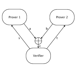
Figure 9.1: A one-round XOR proof system.

Here, we are particularly interested in non-local games. Alice and Bob are allowed to share an arbitrary entangled state $|\Psi\rangle$ to help them win the game. Let $\mathcal{H}^{A}$ and $\mathcal{H}^{B}$ denote the Hilbert spaces of Alice and Bob respectively. The state $|\Psi\rangle\in\mathcal{H}^{A}\otimes\mathcal{H}^{B}$ is part of the quantum strategy that Alice and Bob can agree on beforehand. This means that for each game, Alice and Bob can choose a specific $|\Psi\rangle$ to maximize their chance of success. In addition, Alice and Bob can agree on quantum measurements. For each $s\in S$, Alice has a projective measurement described by $\{X_{s}^{a}\mid a\in A\}$ on $\mathcal{H}^{A}$. For each $t\in T$, Bob has a projective measurement described by $\{Y_{t}^{b}\mid b\in B\}$ on $\mathcal{H}^{B}$. For questions $(s,t)\in S\times T$, Alice performs the measurement corresponding to $s$ on her part of $|\Psi\rangle$ which gives her outcome $a$. Likewise, Bob performs the measurement corresponding to $t$ on his part of $|\Psi\rangle$ with outcome $b$. Both send their outcome, $a$ and $b$, back to the verifier. The probability that Alice and Bob answer $(a,b)\in A\times B$ is then given by

$$\langle\Psi|X_{s}^{a}\otimes Y_{t}^{b}|\Psi\rangle.$$

The probability that Alice and Bob win the game is now given by

$$\Pr[\mbox{Alice and Bob win}]=\sum_{s,t}\pi(s,t)\sum_{a,b}V(a,b|s,t)\langle\Psi|X_{s}^{a}\otimes Y_{t}^{b}|\Psi\rangle.$$ (9.1)

The quantum value $\omega_{q}(G)$ of a game $G$ is the maximum probability over all possible quantum strategies that Alice and Bob win. Recall that XOR game is a game where the value of $V$ only depends on $c=a\oplus b$ and not on $a$ and $b$ independently. For XOR games we write $V(c|s,t)$ instead of $V(a,b|s,t)$. Here, we are only interested in the case that $a\in\{0,1\}$ and $b\in\{0,1\}$ and XOR games. Alice and Bob’s measurements are then described by $\{X_{s}^{0},X_{s}^{1}\}$ for $s\in S$ and $\{Y_{t}^{0},Y_{t}^{1}\}$ for $t\in T$ respectively. Note that $X_{s}^{0}+X_{s}^{1}=\mathbb{I}$ and $Y_{t}^{0}+Y_{t}^{0}=\mathbb{I}$ and thus these measurements can be expressed in the form of observables $X_{s}$ and $Y_{t}$ with eigenvalues $\pm 1$: $X_{s}=X_{s}^{0}-X_{s}^{1}$ and $Y_{t}=Y_{t}^{0}-Y_{t}^{1}$. Recall from Chapter 6.3.2 that Tsirelson [Tsi80, Tsi87] has shown that for any $|\Psi\rangle\in\mathcal{H}^{A}\otimes\mathcal{H}^{B}$ there exists real unit vectors $x_{s},y_{t}\in\mathbb{R}^{N}$ with $N=|S|+|T|$ such that $\langle\Psi|X_{s}\otimes Y_{t}|\Psi\rangle=\langle{x_{s}}|{y_{t}}\rangle$. It is then easy to see from Eq. (9.1) that for XOR games we can express the maximum winning probability as

$$\omega_{q}(G)=\max_{x_{s},y_{t}}\frac{1}{2}\sum_{s,t}\pi(s,t)\sum_{c}V(c|s,t)\left(1+(-1)^{c}\langle{x_{s}}|{y_{t}}\rangle\right),$$ (9.2)

where the maximization is taken over all unit vectors $x_{s},y_{t}\in\mathbb{R}^{N}$.

9.2.2 Multiple classical provers

It is well known [CHTW04a, FL92], that two-prover one-round interactive proof systems with classical communication can be modeled as (non-local) games. Here, Alice and Bob take the role of the two provers. The verifier now poses questions $s$ and $t$, and evaluates the resulting answers. A proof system associates with each string $x$ a game $G_{x}$, where $\omega(G_{x})$ determines the probability that the verifier accepts (and thus concludes $x\in L$). The string $x$, and thus the nature of the game $G_{x}$ is known to both the verifier and the provers. Ideally, for all $x\in L$ the value of $\omega(G_{x})$ is close to one, and for $x\notin L$ the value of $\omega(G_{x})$ is close to zero. It is possible to extend the game model for MIP[2] to use a randomized predicate for the acceptance predicate $V$. This corresponds to $V$ taking an extra input string chosen at random by the verifier. However, known applications of MIP[2] proof systems do not require this extension [Fei95]. Our argument in Section 9.3 can easily be extended to deal with randomized predicates. Since $V$ is not a randomized predicate in [CHTW04a], we follow this approach.

We concentrate on proof systems involving two provers, one round of communication, and single-bit answers. The provers are computationally unbounded, but limited by the laws of quantum physics. However, the verifier is probabilistic polynomial time bounded. As defined by Cleve, Høyer, Toner and Watrous [CHTW04a],

Definition 9.2.1.

For $0\leq s<c\leq 1$, let $\oplus\mbox{MIP}_{c,s}[2]$ denote the class of all languages $L$ recognized by a classical two-prover interactive proof system of the following form:

• They operate in one round, each prover sends a single bit in response to the verifier’s question, and the verifier’s decision is a function of the parity of those two bits.

• If $x\in L$ then there exists a strategy for the provers for which the probability that the verifier accepts is at least $c$ (the completeness probability).

• If $x\notin L$ then, whatever strategy the two provers follow, the probability that the verifier accepts is at most $s$ (the soundness probability).

Definition 9.2.2.

For $0\leq s<c\leq 1$, let $\oplus\mbox{MIP}^{*}_{c,s}[2]$ denote the class corresponding to a modified version of the previous definition: all communication remains classical, but the provers may share prior quantum entanglement, which may depend on $x$, and perform quantum measurements.

We generally omit indices $c$, $s$, unless they are explicitly relevant.

In Chapter 7, we discussed how to find the optimal strategies for XOR-games. In particular, we saw that we can determine the optimal value of $\omega_{q}(G_{x})$ in time exponential in $\min(|S|,|T|)$ using semidefinite programming. This implies immediately that $\oplus\mbox{MIP}^{*}\subseteq\mbox{EXP}$, as was shown by Cleve, Høyer, Toner and Watrous [CHTW04a] during their presentation at CCC’04. Here, we show something stronger, namely that $\oplus\mbox{MIP}^{*}\subseteq\mbox{QIP(2)}$.

9.2.3 A single quantum prover

Instead of two classical provers, we can also consider a system consisting of a single quantum prover $P_{q}$ and a quantum polynomial time verifier $V_{q}$ as defined by Watrous [Wat99]. Again, the quantum prover $P_{q}$ is computationally unbounded, however, he is limited by the laws of quantum physics. The verifier and the prover can communicate over a quantum channel. In this thesis, we are only interested in one round quantum interactive proof systems: the verifier sends a single quantum message to the prover, who responds with a quantum answer. We here express the definition of $\mbox{QIP}(2)$ [Wat99] in a form similar to the definition of $\oplus\mbox{MIP}^{*}$:

Definition 9.2.3.

Let $\mbox{QIP}(2,c,s)$ denote the class of all languages $L$ recognized by a quantum one-prover one-round interactive proof system of the following form:

• If $x\in L$ then there exists a strategy for the quantum prover for which the probability that the verifier accepts is at least $c$.

• If $x\notin L$ then, whatever strategy the quantum prover follows, the probability that the quantum verifier accepts is at most $s$.

9.3 Simulating two classical provers with one quantum prover

We now show that an interactive proof system where the verifier bases his decision only on the XOR of two binary answers is in fact no more powerful than a system based on a single quantum prover. The main idea behind our proof is to combine two classical queries into one quantum query, and thereby simulate the classical proof system with a single quantum prover. Similar techniques have been used to prove results about classical locally decodable codes [KW03, WdW05]. Recall that the two provers can use an arbitrary entangled state as part of their strategy.

For our proof we make use of the fact that we can write the optimal value of the game as in Eq. (9.2).

Theorem 9.3.1.

For all $s$ and $c$ such that $0\leq s<c\leq 1$, $\oplus\mbox{\emph{MIP}}_{c,s}^{*}[2]\subseteq\mbox{\emph{QIP}}(2,c,s)$.

Proof 9.3.2.

Let $L\in\oplus\mbox{MIP}_{c,s}^{*}[2]$ and let $V_{e}$ be a verifier witnessing this fact. Let $P_{e}^{1}$ (Alice) and $P_{e}^{2}$ (Bob) denote the two provers sharing entanglement. Fix an input string $x$. As mentioned above, interactive proof systems can be modeled as games indexed by the string $x$. It is therefore sufficient to show that there exists a verifier $V_{q}$ and a quantum prover $P_{q}$, such that $\omega_{sim}(G_{x})=\omega_{q}(G_{x})$, where $\omega_{sim}(G_{x})$ is the value of the simulated game.

Let $s$,$t$ be the questions that $V_{e}$ sends to the two provers $P_{e}^{1}$ and $P_{e}^{2}$ in the original game. The new verifier $V_{q}$ now constructs the following state in $\mathcal{V}\otimes\mathcal{M}$

$$|\Phi_{init}\rangle=\frac{1}{\sqrt{2}}(\underbrace{|0\rangle}_{\mathcal{V}}\underbrace{|0\rangle|s\rangle}_{\mathcal{M}}+\underbrace{|1\rangle}_{\mathcal{V}}\underbrace{|1\rangle|t\rangle}_{\mathcal{M}}),$$

and sends register $\mathcal{M}$ to the single quantum prover $P_{q}$.

We first consider the honest strategy of the prover. Let $a$ and $b$ denote the answers of the two classical provers to questions $s$ and $t$ respectively. The quantum prover now transforms the state to

$$|\Phi_{honest}\rangle=\frac{1}{\sqrt{2}}((-1)^{a}\underbrace{|0\rangle}_{\mathcal{V}}\underbrace{|0\rangle|s\rangle}_{\mathcal{M}}+(-1)^{b}\underbrace{|1\rangle}_{\mathcal{V}}\underbrace{|1\rangle|t\rangle}_{\mathcal{M}}),$$

and returns register $\mathcal{M}$ back to the verifier. The verifier $V_{q}$ now performs a measurement on $\mathcal{V}\otimes\mathcal{M}$ described by the following projectors

$$P_{0} = |\Psi^{+}_{st}\rangle\langle\Psi^{+}_{st}|\otimes I$$

$$P_{1} = |\Psi^{-}_{st}\rangle\langle\Psi^{-}_{st}|\otimes I$$

$$P_{reject} = I-P_{0}-P_{1},$$

where $|\Psi^{\pm}_{st}\rangle=(|0\rangle|0\rangle|s\rangle\pm|1\rangle|1\rangle|t\rangle)/\sqrt{2}$. If he obtains outcome “reject”, he immediately aborts and concludes that the quantum prover is cheating. If he obtains outcome $m\in\{0,1\}$, the verifier concludes that $c=a\oplus b=m$. Note that $\Pr[m=a\oplus b|s,t]=\langle\Phi_{honest}|P_{a\oplus b}|\Phi_{honest}\rangle=1$, so the verifier can reconstruct the answer perfectly.

We now consider the case of a dishonest prover. In order to convince the verifier, the prover applies a transformation on $\mathcal{M}\otimes\mathcal{P}$ and send register $\mathcal{M}$ back to the verifier. We show that for any such transformation the value of the resulting game is at most $\omega_{q}(G_{x})$: Note that the state of the total system in $\mathcal{V}\otimes\mathcal{M}\otimes\mathcal{P}$ can now be described as

$$|\Phi_{dish}\rangle=\frac{1}{\sqrt{2}}(|0\rangle|\phi_{s}\rangle+|1\rangle|\phi_{t}\rangle)$$

where $|\phi_{s}\rangle=\sum_{u\in S^{\prime}\cup T^{\prime}}|u\rangle|\alpha_{u}^{s}\rangle$ and $|\phi_{t}\rangle=\sum_{v\in S^{\prime}\cup T^{\prime}}|v\rangle|\beta_{v}^{t}\rangle$ with $S^{\prime}=\{0s|s\in S\}$ and $T^{\prime}=\{1t|t\in T\}$. Any transformation employed by the prover can be described this way. We now have that

$$\Pr[m=0|s,t]=\langle\Phi_{dish}|P_{0}|\Phi_{dish}\rangle = \frac{1}{4}(\langle{\alpha_{s}^{s}}|{\alpha_{s}^{s}}\rangle+\langle{\beta_{t}^{t}}|{\beta^{t}_{t}}\rangle)+\frac{1}{2}\Re(\langle{\alpha_{s}^{s}}|{\beta_{t}^{t}}\rangle)$$ (9.3)

$$\Pr[m=1|s,t]=\langle\Phi_{dish}|P_{1}|\Phi_{dish}\rangle = \frac{1}{4}(\langle{\alpha_{s}^{s}}|{\alpha_{s}^{s}}\rangle+\langle{\beta_{t}^{t}}|{\beta^{t}_{t}}\rangle)-\frac{1}{2}\Re(\langle{\alpha_{s}^{s}}|{\beta_{t}^{t}}\rangle)$$ (9.4)

The probability that the prover wins is given by

$$\Pr[\mbox{Prover wins}]=\sum_{s,t}\pi(s,t)\sum_{c\in\{0,1\}}V(c|s,t)\Pr[m=c|s,t].$$

The prover will try to maximize his chance of success by maximizing $\Pr[m=0|s,t]$ or $\Pr[m=1|s,t]$. We can therefore restrict ourselves to considering real unit vectors for which $\langle{\alpha_{s}^{s}}|{\alpha_{s}^{s}}\rangle=1$ and $\langle{\beta_{t}^{t}}|{\beta_{t}^{t}}\rangle=1$, as the dimension of our vectors is directly determined by their number. Hence, we may also assume that $|\alpha_{s}^{s^{\prime}}\rangle=0$ iff $s\neq s^{\prime}$ and $|\beta_{t}^{t^{\prime}}\rangle=0$ iff $t\neq t^{\prime}$: any other strategy can lead to rejection and thus to a lower probability of success. By substituting into Eqs. (9.3) and (9.4), it follows that the probability that the quantum prover wins the game (when he avoids rejection) is

$$\frac{1}{2}\sum_{s,t,c}\pi(s,t)V(c|s,t)(1+(-1)^{c}\langle{\alpha_{s}^{s}}|{\beta_{t}^{t}}\rangle).$$ (9.5)

In order to convince the verifier, the prover’s goal is to choose real vectors $|\alpha_{s}^{s}\rangle$ and $|\beta_{t}^{t}\rangle$ which maximize Eq. (9.5). Since in $|\phi_{s}\rangle$ and $|\phi_{t}\rangle$ we sum over $|S^{\prime}|+|T^{\prime}|=|S|+|T|$ elements respectively, the dimension of $\mathcal{P}$ need not exceed $N=|S|+|T|$. Thus, it is sufficient to restrict the maximization to vectors in $\mathbb{R}^{|S|+|T|}$. Given Eq. (9.5), we thus have

$$\omega_{sim}(G_{x})=\max_{\alpha_{s}^{s},\beta_{t}^{t}}\frac{1}{2}\sum_{s,t,c}\pi(s,t)V(c|s,t)(1+(-1)^{c}\langle{\alpha_{s}^{s}}|{\beta_{t}^{t}}\rangle),$$

where the maximization is taken over vectors $\{\alpha_{s}^{s}\in\mathbb{R}^{N}:s\in S\}$, and $\{\beta_{t}^{t}\in\mathbb{R}^{N}:t\in T\}$. However, we know from Eq. (9.2) that

$$\omega_{q}(G_{x})=\max_{x_{s},y_{t}}\frac{1}{2}\sum_{s,t,c}\pi(s,t)V(c|s,t)(1+(-1)^{c}\langle{x_{s}}|{y_{t}}\rangle)$$

where the maximization is taken over unit vectors $\{x_{s}\in\mathbb{R}^{N}:s\in S\}$ and $\{y_{t}\in\mathbb{R}^{N}:t\in T\}$. We thus have

$$\omega_{sim}(G_{x})=\omega_{q}(G_{x})$$

which completes our proof.

Corollary 9.3.3.

For all $s$ and $c$ such that $0\leq s<c\leq 1$, $\oplus\mbox{\emph{MIP}}_{c,s}^{*}[2]\subseteq\mbox{\emph{EXP}}$.

Proof 9.3.4.

This follows directly from Theorem 9.3.1 and the result that $\mbox{QIP(2)}\subseteq\mbox{EXP}$ [KW00].

9.4 Conclusion

As we have shown, the strength of classical systems can be weakened considerably in the presence of entanglement. In our example above, we showed that the systems can be weakened so much that all space-like separation is lost: we saw that two classical parties with entanglement are as powerful as a single quantum party.

It would be interesting to show that this result also holds for a proof system where the verifier is not restricted to computing the XOR of both answers, but some other Boolean function. However, the approach based on vectors from Tsirelson’s results does not work for binary games. Whereas it is easy to construct a single quantum query which allows the verifier to compute an arbitrary function of the two binary answers with some advantage, it thus remains unclear how the value of the resulting game is related to the value of a binary game. Furthermore, mere classical tricks trying to obtain the value of a binary function from XOR itself seem to confer extra cheating power to the provers.

Examples of non-local games with longer answers [CHTW04a], such as the Kochen-Specker or the Magic Square game, seem to make it even easier for the provers to cheat by taking advantage of their entangled state. Furthermore, existing proofs that $\mbox{MIP}=\mbox{NEXP}$ break down if the provers share entanglement. It is therefore an open question whether $\mbox{MIP}^{*}=\mbox{NEXP}$ or, $\mbox{MIP}^{*}\subseteq\mbox{EXP}$.

As described, non-locality experiments between two space-like separated observers, Alice and Bob, can be cast in the form of non-local games. For example, the experiment based on the well known CHSH inequality [CHSH69], is a non-local game with binary answers of which the verifier computes the XOR [CHTW04a]. Our result implies that this non-local game can be simulated in superposition by a single prover/observer: Any strategy that Alice and Bob might employ in the non-local game can be mirrored by the single prover in the constructed “superposition game”, and also vice versa, due to Tsirelson’s constructions [Tsi80, Tsi87] mentioned earlier. This means that the “superposition game” corresponding to the non-local CHSH game is in fact limited by Tsirelson’s inequality [Tsi80], even though it itself has no non-local character. Whereas this may be purely coincidental, it would be interesting to know its physical interpretation, if any. Perhaps it may be interesting to ask whether Tsirelson-type inequalities have any consequences on local computations in general, beyond the scope of these very limited games.

Part IV Consequences for Crytography

Chapter 10 Limitations

Finally, we turn our attention to cryptographic protocols directly. As we saw in Chapter 1, it is impossible to implement bit commitment even in the quantum setting! In the face of the negative results, what can we still hope to achieve?

10.1 Introduction

Here, we consider the task of committing to an entire string of $n$ bits at once when both the honest player and the adversary have unbounded resources. Since perfect bit commitment is impossible, perfect bit string commitment is clearly impossible as well. Curiously, however, we can still make interesting statements in the quantum setting, if we give both Alice and Bob a limited ability to cheat. That is, we allow Alice to change her mind about the committed string within certain limited parameters, and allow Bob to gain some information about the committed string. It turns out that it matters crucially how we measure Bob’s information gain.

First, we introduce a framework for the classification of bit string commitments in terms of the length $n$ of the string, Alice’s ability to cheat on at most $a$ bits and Bob’s ability to acquire at most $b$ bits of information before the reveal phase. We say that Alice can cheat on $a$ bits if she can reveal up to $2^{a}$ strings successfully. Bob’s security definition is crucial to our investigation: If $b$ determines a bound on his probability to guess Alice’s string, then we prove that $a+b$ is at least $n$. This implies that the trivial protocol, where Alice’s commitment consists of sending $b$ bits of her string to Bob, is optimal. If, however, $b$ is a bound on the accessible information that the quantum states contain about Alice’s string, then we show that non-trivial schemes exist. More precisely, we construct schemes with $a=4\log n+O(1)$ and $b=4$. This is impossible classically. We also present a simple, implementable, protocol, that achieves $a=1$ and $b=n/2$. This protocol can furthermore be made cheat-sensitive. Quantum commitments of strings have previously been considered by Kent [Ken03], who pointed out that in the quantum world useful bit string commitments could be possible despite the no-go theorem for bit commitment. His scenario differs significantly from ours and imposes an additional constraint, which is not present in our work: Alice does not commit to a superposition of strings.

10.2 Preliminaries

10.2.1 Definitions

We first formalize the notion of quantum string commitments in a quantum setting.

Definition 10.2.1.

An $(n,a,b)$-Quantum Bit String Commitment (QBSC) is a quantum communication protocol between two parties, Alice (the committer) and Bob (the receiver), which consists of two phases:

• (Commit Phase) Assume that both parties are honest. Alice chooses a string $x\in\{0,1\}^{n}$ with probability $p_{x}$. Alice and Bob communicate and at the end Bob holds state $\rho_{x}$.

• (Reveal Phase) If both parties are honest, Alice and Bob communicate and at the end Bob outputs $x$. Bob accepts.

We have the following two security requirements:

• (Concealing) If Alice is honest, then for any strategy of Bob

  $$\sum_{x\in\{0,1\}^{n}}p^{B}_{x|x}\leq 2^{b},$$

  where $p^{B}_{x|x}$ is the probability that Bob correctly guesses $x$ before the reveal phase.

• (Binding) If Bob is honest, then for any strategy of Alice

  $$\sum_{x\in\{0,1\}^{n}}p^{A}_{x}\leq 2^{a},$$

  where $p^{A}_{x}$ is the probability that Alice successfully reveals $x$ (Bob accepts the opening of $x$).

Bob thereby accepts the opening of a string $x$, if he performs a test depending on the individual protocol to check Alice’s honesty and concludes that she was indeed honest. Note that quantumly, Alice can always commit to a superposition of different strings without being detected. Thus even for a perfectly binding bit string commitment (i.e. $a=0$) we only demand that $\sum_{x\in\{0,1\}^{n}}p^{A}_{x}\leq 1$, whereas classically one wants that $p^{A}_{x^{\prime}}=\delta_{x,x^{\prime}}$. Note that our concealing definition reflects Bob’s a priori knowledge about $x$. We choose an a priori uniform distribution (i.e. $p_{x}=2^{-n}$) for $(n,a,b)$-QBSCs, which naturally comes from the fact that we consider $n$-bit strings. A generalization to any $(P_{X},a,b)$-QBSC where $P_{X}$ is an arbitrary distribution is possible but omitted in order not to obscure our main line of argument.

Instead of Bob’s guessing probability, one can take any information measure $B$ to express the security against Bob. In general, we consider an $(n,a,b)$-$\mbox{QBSC}_{B}$ where the new Concealing-condition reads

• (General Concealing) If Alice is honest, then for any ensemble $\mathcal{E}=\{p_{x},\rho_{x}\}$ that Bob can obtain by a cheating strategy $B(\mathcal{E})\leq b$.

Later, we will show that for $B$ being the accessible information, non-trivial protocols, i.e. protocols with $a+b\ll n$, do exist. Recall that the accessible information was defined in Section 2.3.2 as $\mathcal{I}_{acc}(\mathcal{E})=\max_{M}I(X,Y)$, where $P_{X}$ is the prior distribution of the random variable $X$, $Y$ is the random variable of the outcome of Bob’s measurement on $\mathcal{E}$, and the maximization is taken over all measurements $M$.

10.2.2 Model

We work in the model of two-party non-relativistic quantum protocols of Yao [Yao95], simplified by Lo and Chau [LC97] which is usually adopted in this context. Here, any two-party quantum protocol can be regarded as a pair of quantum machines (Alice and Bob), interacting through a quantum channel. Consider the product of three Hilbert spaces $\mathcal{H}_{A}$, $\mathcal{H}_{B}$ and $\mathcal{H}_{C}$ of bounded dimensions, representing the Hilbert spaces of Alice’s and Bob’s machines and the channel, respectively. Without loss of generality, we assume that each machine is initially in a specified pure state. Alice and Bob perform a number of rounds of communication over the channel. Each such round can be modeled as a unitary transformation on $\mathcal{H}_{A}\otimes\mathcal{H}_{C}$ and $\mathcal{H}_{B}\otimes\mathcal{H}_{C}$ respectively. Since the protocol is known to both Alice and Bob, they know the set of possible unitary transformations used in the protocol. We assume that Alice and Bob are in possession of both a quantum computer and a quantum storage device. This enables them to add ancillae to the quantum machine and use reversible unitary operations to replace measurements. The state of this ancilla can then be read off only at the end of the protocol, and by doing so, Alice and Bob can effectively delay any measurements until the very end. The resulting protocol will be equivalent to the original and thus we can limit ourselves to protocols where both parties only measure at the very end. Moreover, any classical computation or communication that may occur can be simulated by a quantum computer.

10.2.3 Tools

We now gather the essential ingredients for our proof. First, we now show that every $(n,a,b)$-QBSC is an $(n,a,b)$-$\mbox{QBSC}_{\xi}$. The security measure $\xi(\mathcal{E})$ is defined by

$$\xi(\mathcal{E}):=n-H_{2}(\rho_{AB}|\rho),$$ (10.1)

where $\rho_{AB}=\sum_{x}p_{x}|x\rangle\langle x|\otimes\rho_{x}$ and $\rho=\sum_{x}p_{x}\rho_{x}$ are only dependent on the ensemble $\mathcal{E}=\{p_{x},\rho_{x}\}$. $H_{2}(\cdot|\cdot)$ is an entropic quantity defined in [Ren05]

$$H_{2}(\rho_{AB}|\rho):=-\log\mbox{\rm Tr}\left(\left[\mathbb{I}\otimes\rho^{-\frac{1}{2}})\rho_{AB}\right]^{2}\right).$$

Interestingly, this quantity is directly connected to Bob’s maximal average probability of successfully guessing the string:

Lemma 10.2.2.

Bob’s maximal average probability of successfully guessing the committed string, i.e. $\sup_{M}\sum_{x}p_{x}p^{B,M}_{x|x}$ where $M=\{M_{x}\}$ ranges over all measurements and $p^{B,M}_{y|x}=\mbox{\rm Tr}(M_{y}\rho_{x})$ is the conditional probability of outputting $y$ given $\rho_{x}$, obeys

$$\sup_{M}\sum_{x}p_{x}p^{B,M}_{x|x}\geq 2^{-H_{2}(\rho_{AB}|\rho)}.$$

Proof 10.2.3.

By definition, the maximum average guessing probability is lower bounded by the average guessing probability for a particular measurement strategy. We choose the square-root measurement which has operators

$$M_{x}=p_{x}\rho^{-\frac{1}{2}}\rho_{x}\rho^{-\frac{1}{2}}.$$

We use $p^{B}_{x|x}=\mbox{\rm Tr}(M_{x}\rho_{x})$ to denote the probability that Bob guesses $x$ given $\rho_{x}$, hence

$$\log\sum_{x}p_{x}p^{B,\max}_{x|x} \geq \log\sum_{x}p_{x}^{2}\mbox{\rm Tr}(\rho^{-\frac{1}{2}}\rho_{x}\rho^{-\frac{1}{2}}\rho_{x})$$

$$= \log\mbox{\rm Tr}\left(\sum_{x}p_{x}^{2}|x\rangle\langle x|\otimes\rho^{-\frac{1}{2}}\rho_{x}\rho^{-\frac{1}{2}}\rho_{x}\right)$$

$$= \log\mbox{\rm Tr}\left(\left[(\mathbb{I}\otimes\rho^{-\frac{1}{2}})\rho_{AB}\right]^{2}\right)$$

$$= -H_{2}(\rho_{AB}|\rho)$$

Related estimates were derived in [BK02].

Furthermore, we make use of the following theorem, known as privacy amplification against a quantum adversary with two-universal hash functions, which we state in a form that is most convenient for our purposes in this chapter. A class $\mathcal{F}$ of functions $f:\{0,1\}^{n}\rightarrow\{0,1\}^{\ell}$ is thereby called two-universal if for all $x\neq y\in\{0,1\}^{n}$ and for uniformly at random chosen $f\in\mathcal{F}$ we have $\Pr[f(x)=f(y)]\leq 2^{-\ell}$. For example, the set of all affine functions. from $\{0,1\}^{n}$ to $\{0,1\}^{\ell}$ is two-universal [CW79]. The following theorem expresses how hash functions can decrease Bob’s knowledge about a random variable when he holds some quantum information. In our case, Bob will hold some quantum memory and privacy amplification is used to find Alice’s attack.

Theorem 10.2.4 (Th. 5.5.1 in [Ren05] (see also [KMR05])).

Let $\mathcal{G}$ be a class of two-universal hash functions from $\{0,1\}^{n}$ to $\{0,1\}^{s}$. Application of $g\in\mathcal{G}$ to the random variable $X$ maps the ensemble $\mathcal{E}=\{p_{x},\rho_{x}\}$ to $\mathcal{E}_{g}=\{q^{g}_{y},\sigma^{g}_{y}\}$ with probabilities $q^{g}_{y}=\sum_{x\in g^{-1}(y)}p_{x}$ and quantum states $\sigma^{g}_{y}=\sum_{x\in g^{-1}(y)}p_{x}\rho_{x}$. Then

$$\frac{1}{|\mathcal{G}|}\sum_{g\in\mathcal{G}}d(\mathcal{E}_{g})\leq\frac{1}{2}2^{-\frac{1}{2}[H_{2}(\rho_{AB}|\rho)-s]},$$ (10.2)

where $d(\mathcal{E}):=D\big{(}\sum_{x}p_{x}|x\rangle\langle x|\otimes\rho_{x},\mathbb{I}/2^{n}\otimes\rho\big{)}$ (and similarly for $d(\mathcal{E}_{g})$).

Finally, the following reasoning that is used to prove the impossibility of quantum bit commitment [LC97, May96b] will be essential: Suppose $\rho_{0}$ and $\rho_{1}$ are density operators that correspond to the state of Bob’s system if Alice committed a “0” or a “1” respectively. Let $|\phi_{0}\rangle$ and $|\phi_{1}\rangle$ be the corresponding purifications on the joint system of Alice and Bob: Alice holds the purification of $\rho_{0}$ and $\rho_{1}$. If $\rho_{0}$ equals $\rho_{1}$ then Alice can find a local unitary transformation $U$ that Alice can apply to her part of the system such that $|\phi_{1}\rangle=U\otimes\mathbb{I}|\phi_{0}\rangle$. This enables Alice to change the total state from $|\phi_{0}\rangle$ to $|\phi_{1}\rangle$ and thus cheat using entanglement! This reasoning also holds in an approximate sense [May96b], here used in the following form:

Lemma 10.2.5.

Let $D(\rho_{0},\rho_{1})\leq\epsilon$ and assume that the bit-commitment protocol is error-free if both parties are honest. Then there exists a method for Alice to cheat such that the probability of successfully revealing a $0$ during the reveal phase, given that she honestly committed herself to a $1$ during the commit phase, is at least $1-\sqrt{2\epsilon}$.

Proof 10.2.6.

$D(\rho_{0},\rho_{1})\leq\epsilon$ implies $\max_{U}|\langle\phi_{0}|U\otimes\mathbb{I}|\phi_{1}\rangle|\geq 1-\varepsilon$ by Uhlmann’s theorem [Uhl76]. Here, $|\phi_{0}\rangle$ and $|\phi_{1}\rangle$ correspond to the joint states after the commit phase if Alice committed to a ’0’ or ’1’ respectively where the maximization ranges over all unitaries $U$ on Alice’s (i.e. the purification) side. Let $|\psi_{0}\rangle=U\otimes\mathbb{I}|\phi_{1}\rangle$ for a $U$ achieving the maximization, be the state that Alice prepares by applying $U$ to the state on her side when she wants to reveal a ’1’, given a prior honest commitment to ’0’. We then have

$$D(|\phi_{0}\rangle\langle\phi_{0}|,|\psi_{0}\rangle\langle\psi_{0}|) = \sqrt{1-|\langle\phi_{0}|\psi_{0}\rangle|^{2}}$$

$$\leq \sqrt{1-(1-\epsilon)^{2}}$$

$$\leq \sqrt{2\epsilon}.$$

If Bob is honest, the reveal phase can be regarded as a measurement resulting in a distribution $P_{Y}$ (or $P_{Z}$) if $|\phi_{0}\rangle$ (or $|\psi_{0}\rangle$) was the state before the reveal phase. The random variables $Y$ and $Z$ can take values $\{0,1\}$ (corresponding to the opened bit) or the value ‘reject (r)’. Since the trace distance does not increase under measurements, $D(P_{Y},P_{Z})\leq D(|\phi_{0}\rangle\langle\phi_{0}|,|\psi_{0}\rangle\langle\psi_{0}|)\leq\sqrt{2\epsilon}$. Hence $\frac{1}{2}(|P_{Y}(0)-P_{Z}(0)|+|P_{Y}(1)-P_{Z}(1)|+|P_{Y}(r)-P_{Z}(r)|)\leq\sqrt{2\epsilon}$. Since $|\phi_{0}\rangle$ corresponds to Alice’s honest commitment to $0$ we have $P_{Y}(0)=1$, $P_{Y}(1)=P_{Y}(r)=0$ and hence $P_{Z}(0)\geq 1-\sqrt{2\epsilon}$.

10.3 Impossibility
of quantum string commitments

As we saw above, any $(n,a,b)$-QBSC is also an $(n,a,b)$-$\mbox{QBSC}_{\xi}$ with the security measure $\xi(\mathcal{E})$ defined in Eq. (10.1). To prove our impossibility result we now prove that an $(n,a,b)$-$\mbox{QBSC}_{\xi}$ can only exist for values $a$, $b$ and $n$ obeying $a+b+c\geq n$, where $c$ is a small constant independent of $a$, $b$ and $n$. This in turn implies the impossibility of an $(n,a,b)$-QBSC for such parameters. Finally, we show that if we execute the protocol many times in parallel, the protocol can only be secure if $a+b\geq n$.

The intuition behind our proof is simple: To cheat, Alice first chooses a two-universal hash function $g$. She then commits to a superposition of all strings for which $g(x)=y$ for a specific $y$. We now know from the privacy amplification theorem above, that even though Bob may gain some knowledge about $x$, he is entirely ignorant about $y$. But then Alice can change her mind and reveal a string from a different set of strings for which $g(x)=y^{\prime}$ with $y\neq y^{\prime}$ as we saw above! The following figure illustrates this idea.

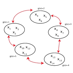
Figure 10.1: Moving from a set of string with $g(x)=y$ to a set of strings with $g(x)=(y\mod 5)+1$.

Theorem 10.3.1.

$(n,a,b)$-$\mbox{QBSC}_{\xi}$ schemes with $a+b+c<n$ do not exist, where $c=5\log 5-4\approx 7.61$ is a constant.

Proof 10.3.2.

Consider an $(n,a,b)$-$\mbox{QBSC}_{\xi}$ and the case where both Alice and Bob are honest. Alice committed to $x$. We denote the joint state of the system Alice-Bob-Channel $\mathcal{H}_{A}\otimes\mathcal{H}_{B}\otimes\mathcal{H}_{C}$ after the commit phase by $|\phi_{x}\rangle$ for input state $|x\rangle$. Let $\rho_{x}$ be Bob’s reduced density matrix, and let $\mathcal{E}=\{p_{x},\rho_{x}\}$ where $p_{x}=2^{-n}$.

Assuming that Bob is honest, we will give a cheating strategy for Alice in the case where $a+b+5\log 5-4<n$. The strategy will depend on the two-universal hash function $g:\mathcal{X}=\{0,1\}^{n}\rightarrow\mathcal{Y}=\{0,1\}^{n-m}$, for appropriately chosen $m$. Alice picks a $y\in\mathcal{Y}$ and constructs the state $(\sum_{x\in g^{-1}(y)}|x\rangle|x\rangle)/\sqrt{|g^{-1}(y)|}$. She then gives the second half of this state as input to the protocol and stays honest for the rest of the commit phase. The joint state of Alice and Bob at the end of the commit phase is thus $|\psi^{g}_{y}\rangle=(\sum_{x\in g^{-1}(y)}|x\rangle|\phi_{x}\rangle)/\sqrt{|g^{-1}(y)|}$. The reduced states on Bob’s side are $\sigma^{g}_{y}=\frac{1}{q^{g}_{y}}\sum_{x\in g^{-1}(y)}p_{x}\rho_{x}$ with probability $q^{g}_{y}=\sum_{x\in g^{-1}(y)}p_{x}$. We denote this ensemble by $\mathcal{E}_{g}$. Let $\sigma^{g}=\sum_{y}q^{g}_{y}\sigma^{g}_{y}$.

We now apply Theorem 10.2.4 with $s=n-m$ and $\xi(\mathcal{E})\leq b$ and obtain $\frac{1}{|\mathcal{G}|}\sum_{g\in\mathcal{G}}d(\mathcal{E}_{g})\leq\varepsilon$ where $\varepsilon=\frac{1}{2}2^{-\frac{1}{2}(m-b)}$. Hence, there is at least one $g$ such that $d(\mathcal{E}_{g})\leq\varepsilon$. Intuitively, this means that Bob knows only very little about the value of $g(x)$. This $g$ defines Alice’s cheating strategy. It is straightforward to verify that $d(\mathcal{E}_{g})\leq\varepsilon$ implies

$$2^{-(n-m)}\sum_{y\in\mathcal{Y}}D(\sigma^{g},\sigma^{g}_{y})\leq 2\varepsilon.$$ (10.3)

We therefore assume without loss of generality that Alice chooses $y_{0}\in\mathcal{Y}$ with $D(\sigma^{g}_{y_{0}},\sigma^{g})\leq 2\varepsilon$.

We first observe that the probability to successfully reveal some $x$ in $g^{-1}(y)$ given $|\psi^{g}_{y}\rangle$ is one. We say that Alice reveals $y$ if she reveals an $x$ such that $y=g(x)$. We then also have that the probability for Alice to reveal $y$ given $|\psi^{g}_{y}\rangle$ successfully is one. Let $\tilde{p}_{x}$ and $\tilde{q}^{g}_{y}$ denote the probabilities to successfully reveal $x$ and $y$ respectively and $\tilde{p}^{g}_{x|y}$ be the conditional probability to successfully reveal $x$, given $y$. We have

$$\sum_{x}\tilde{p}_{x}=\sum_{y}\tilde{q}^{g}_{y}\sum_{x\in g^{-1}(y)}\tilde{p}^{g}_{x|y}\geq\sum_{y}\tilde{q}^{g}_{y},$$

where the inequality follows from our observation above.

As in the impossibility proof of bit commitment, Alice can now transform $|\psi^{g}_{y_{0}}\rangle$ approximately into $|\psi^{g}_{y}\rangle$ if $\sigma^{g}_{y_{0}}$ is sufficiently close to $\sigma^{g}_{y}$ by using only local transformations on her part. Indeed, Lemma 10.2.5 tells us how to bound the probability of revealing $y$, given that the state was really $|\psi_{y_{0}}\rangle$. Since this reasoning applies to all $y$, on average, we have

$$\sum_{y}\tilde{q}^{g}_{y} \geq \sum_{y}\left(1-\sqrt{2}\sqrt{D(\sigma^{g}_{y_{0}},\sigma^{g}_{y})}\right)$$

$$\geq 2^{n-m}-2^{n-m}\sqrt{2}\sqrt{2^{m-n}\sum_{y}D(\sigma^{g}_{y_{0}},\sigma^{g}_{y})}$$

$$\geq 2^{n-m}\left(1-\sqrt{2}\sqrt{2^{m-n}\left(\sum_{y}D(\sigma^{g}_{y_{0}},\sigma^{g})+D(\sigma^{g},\sigma^{g}_{y})\right)}\right)$$

$$\geq 2^{n-m}(1-2\sqrt{2\varepsilon}),$$

where the first inequality follows from Lemma 10.2.5, the second from Jensen’s inequality and the concavity of the square root function, the third from the triangle inequality and the fourth from Eq. (10.3) and $D(\sigma^{g}_{y_{0}},\sigma^{g})\leq 2\varepsilon$. Recall that to be secure against Alice, we require $2^{a}\geq 2^{n-m}(1-2\sqrt{2\varepsilon})$. We insert $\varepsilon=\frac{1}{2}2^{-\frac{1}{2}(m-b)}$, define $m=b+\gamma$ and take the logarithm on both sides to get

$$a+b+\delta\geq n,$$ (10.4)

where $\delta=\gamma-\log(1-2^{-\gamma/4+1})$. Keeping in mind that $1-2^{-\gamma/4+1}>0$ (or equivalently $\gamma>4$), we find that the minimum value of $\delta$ for which Eq. (10.4) is satisfied is $\delta=5\log 5-4$ and arises from $\gamma=4(\log 5-1)$. Thus, no $(n,a,b)$-$\mbox{QBSC}_{\xi}$ with $a+b+5\log 5-4<n$ exists.

It follows immediately that the same restriction holds for an $(n,a,b)$-QBSC:

Corollary 10.3.3.

$(n,a,b)$-QBSC schemes, with $a+b+c<n$ do not exist, where $c=5\log 5-4\approx 7.61$ is a constant.

Proof 10.3.4.

For the uniform distribution $p_{x}=2^{-n}$, we have from the concealing condition that $\sum_{x}p^{B}_{x|x}\leq 2^{b}$, which by Lemma 10.2.2 implies $\xi(\mathcal{E})\leq b$. Thus, a $(n,a,b)$-QBSC is an $(n,a,b)$-$\mbox{QBSC}_{\xi}$ from which the result follows.

Since the constant $c$ does not depend on $a$, $b$ and $n$, multiple parallel executions of the protocol can only be secure if $a+b\geq n$. This follows by considering $m$ parallel executions of the protocol as a single execution with a string of length $mn$.

Corollary 10.3.5.

Let $P$ be an $(n,a,b)$-QBSC with $P^{m}$ an $(mn,ma,mb)$-QBSC. Then $n<a+b+c/m$. In particular, no $(n,a,b)$-QBSC with $a+b<n$ can be executed securely an arbitrary number of times in parallel.

Thus, we can indeed hope to do no better than the trivial protocol. It follows directly from [KMP04] that the results in this section also hold in the presence of superselection rules, where, very informally, quantum actions are restricted to act only on certain subspaces of a larger Hilbert space.

10.4 Possibility

Surprisingly, if one is willing to measure Bob’s ability to learn $x$ using a weaker measure of information, the accessible information, non-trivial protocols become possible. These protocols are based on a discovery known as “locking of classical information in quantum states” which we already encountered in Chapter 5.

The protocol, which we call LOCKCOM($n$, $\mathcal{U}$), uses this effect and is specified by a set $\mathcal{U}=\{U_{1},\ldots,U_{|\mathcal{U}|}\}$ of unitaries. We have

Protocol 1: LOCKCOM($n,\mathcal{U}$) 1: Commit phase: Alice has the string $x\in\{0,1\}^{n}$ and randomly chooses $r\in\{1,\ldots,|\mathcal{U}|\}$. She sends the state $U_{r}|x\rangle$ to Bob, where $U_{r}\in\mathcal{U}$. 2: Reveal phase: Alice announces $r$ and $x$. Bob applies $U_{r}^{\dagger}$ and measures in the computational basis to obtain $x^{\prime}$. He accepts if and only if $x^{\prime}=x$. We now first show that our protocol is secure with respect to Definition 10.2.1 if Alice is dishonest. Note that our proof only depends on the number of unitaries used, and is independent of a concrete instantiation of the protocol.

Lemma 10.4.1.

For any LOCKCOM$(n,\mathcal{U})$ protocol the security against a dishonest Alice is bounded by $2^{a}\leq|\mathcal{U}|$,

Proof 10.4.2.

Let $\tilde{p}_{x}$ denote the probability that Alice reveals $x$ successfully. Then, $\tilde{p}_{x}\leq\sum_{r}\tilde{p}_{x,r}$, where $\tilde{p}_{x,r}$ is the probability that $x$ is accepted by Bob when the reveal information was $r$. Let $\rho$ denote the state of Bob’s system. Summation over $x$ now yields

$$\sum_{x}\tilde{p}_{x} \leq \sum_{x,r}\tilde{p}_{x,r}$$

$$= \sum_{x,r}\mbox{\rm Tr}|x\rangle\langle x|U_{r}^{\dagger}\rho U_{r}$$

$$= \sum_{r}\mbox{\rm Tr}\rho=2^{a}.$$

In order to examine security against a dishonest Bob, we have to consider the actual form of the unitaries. We first show that there do indeed exist interesting protocols. Secondly, we present a simple, implementable, protocol. To see that interesting protocols can exist, let Alice choose a set of $O(n^{4})$ unitaries independently according to the Haar measure (approximately discretized) and announce the resulting set $\mathcal{U}$ to Bob. They then perform LOCKCOM($n,\mathcal{U}$). Following the work of [HLSW04], we now show that this variant is secure against Bob with high probability. That is, there exist $O(n^{4})$ unitaries that bring Bob’s accessible information down to a constant: $\mathcal{I}_{acc}(\mathcal{E})\leq 4$:

Theorem 10.4.3.

For $n\geq 3$, there exist $(n,4\log n+O(1),4)$-$\mbox{QBSC}_{\mathcal{I}_{acc}}$ protocols.

Proof 10.4.4.

Let $\mathcal{U}_{ran}$ denote the set of $m$ randomly chosen bases and consider the LOCKCOM($n,a,b$) scheme using unitaries $\mathcal{U}=\mathcal{U}_{ran}$. Security against Alice is again given by Lemma 10.4.1. We now need to show that this choice of unitaries achieves the desired locking effect and thus security against Bob. Again, let $d=2^{n}$ denote the dimension. As we saw in Section 5.2.2 we have that

$$\mathcal{I}_{acc}(\mathcal{E})\leq\log d+\max_{|\phi\rangle}\sum_{j}\frac{1}{m}H(X_{j}),$$

where $X_{j}$ denotes the outcome of the measurement of $|\phi\rangle$ in basis $j$ and the maximum is taken over all pure states $|\phi\rangle$. According to [HLSW04, Appendix B] there is a constant $C^{\prime}>0$ such that

$$\Pr[\inf_{\phi}\frac{1}{m}\sum_{j=1}^{m}H(X_{j}) \leq (1-\varepsilon)\log d-3]$$

$$\leq \left(\frac{10}{\varepsilon}\right)^{2d}2^{-m\left(\frac{\varepsilon C^{\prime}d}{2(\log d)^{2}}-1\right)},$$

for $d\geq 7$ and $\varepsilon\leq 2/5$. Set $\varepsilon=\frac{1}{\log d}$. The RHS of the above equation then decreases provided that $m>\frac{8}{C^{\prime}}(\log d)^{4}$. Thus with $d=2^{n}$ and $\log m=4\log n+O(1)$, the accessible information of the ensemble corresponding to the commitment is then $\mathcal{I}_{acc}(\mathcal{E})\leq\log d-(1-\varepsilon)\log d+3=\varepsilon\log d+3=4$ for our choice of $\varepsilon$.

Unfortunately, the protocol is inefficient both in terms of computation and communication. It remains open to find an efficient constructive scheme with those parameters.

In contrast, for only two bases, an efficient construction exists and uses the identity and the Hadamard transform as unitaries. For this case, the security of the standard LOCKCOM protocol follows immediately from the locking arguments of Chapter 5. It has been shown that this protocol can be made cheat-sensitive [Chr05].

Theorem 10.4.5.

LOCKCOM($n,1,n/2$) using $\mathcal{U}=\{\mathbb{I}^{\otimes n},H^{\otimes n}\}$ is a $(n,1,n/2)$-$\mbox{QBSC}_{\mathcal{I}_{acc}}$ protocol.

Proof 10.4.6.

The result follows immediately from Lemma 10.4.1 and the fact that by Corollary 5.2.6 $\mathcal{I}_{acc}(\mathcal{E})\leq n/2$ for Bob.

We can thus obtain non-trivial protocols by exploiting the locking effects discussed in Chapter 5. Note, however, that the security parameters are very weak. Indeed, if Alice uses only two possible bases chosen with equal probability then Bob is always able to obtain the encoded string with probability at least $1/2$: he simply guesses the basis and performs the corresponding measurement.

10.5 Conclusion

We have introduced a framework for quantum commitments to a string of bits. Even if we consider string commitments that are weaker than bit commitments, no non-trivial protocols can exist if we choose a very strong measure of security. A property of quantum states known as locking, however, allowed us to propose meaningful protocols for a much weaker security demand. One could extend our method to the case of weak secure function evaluation as was done for the original bit commitment protocol in [Lo97]. After completion of our work, Jain [Jai05] has also shown using a different method that $\mbox{QBSC}_{\chi}$ protocols with $a+16b+31<n$ cannot exist.

A drawback of weakening the security requirement is that LOCKCOM protocols are not necessarily composable. Thus, if LOCKCOM is used as a sub-protocol in a larger protocol, the security of the resulting scheme has to be evaluated on a case by case basis. However, LOCKCOM protocols are secure when executed in parallel. This is a consequence of the definition of Alice’s security parameter and the additivity of the accessible information (see Chapter 2), and sufficient for many cryptographic purposes.

However, two important open questions remain: First, how can we construct efficient protocols using more than two bases? It may be tempting to conclude that we could simply use a larger number of mutually unbiased bases, such as given by the identity and Hadamard transform. Yet, as we saw in Chapter 4 using more mutually unbiased bases does not necessarily lead to a better locking effect and thus better string commitment protocols. Finally, are there any novel applications for this weak quantum string commitment?

Fortunately, it turns out that we can implement protocol with very strong security parameters if we are willing to introduce additional assumptions. We now show how to obtain oblivious transfer from the assumption that qubits are affected by noise during storage.

Chapter 11 Possibilities: Exploiting storage errors

Given the negative results from the last chapter, what can we still hope to achieve? Fortunately, the situation is not quite as bleak if we are taking advantage of the technical limitation that quantum storage is necessarily noisy. Here, the very problem that still prevents us from implementing a quantum computer can actually be turned to our advantage! As we saw in Chapter 1 the primitive of oblivious transfer allows us to implement essentially all cryptographic protocols among two mutually distrustful players, and hence we focus on this primitive.

11.1 Introduction

As outlined in Chapter 1, it was recently shown that secure OT is possible when the receiver Bob has a limited amount of quantum memory [DFSS05, DFR⁺07] at his disposal. Within this ‘bounded-quantum-storage model’ OT can be implemented securely as long as a dishonest receiver Bob can store at most $n/4-O(1)$ qubits coherently, where $n$ is the number of qubits transmitted from Alice to Bob. The problem with this approach is that it assumes an explicit limit on the physical number of qubits (or more precisely, the rank of the adversary’s quantum state). However, at present we do not know of any practical physical situation which enforces such a limit for quantum information. On the other hand it is a fact that currently and in the near-future storing photonic qubits is noisy. We therefore propose an alternative model of noisy-quantum storage inspired by present-day physical implementations: We require no explicit memory bound, but we assume that any qubit that is placed into quantum storage undergoes a certain amount of noise. Here, we take the 1-2 OT protocol from [DFR⁺07] as our starting point, and analyze it in this model. This simple 1-2 OT protocol can be implemented using photonic qubits (using polarization or phase-encoding) with standard BB84 quantum key distribution [BB84, GRTZ02] hardware, only with different classical post-processing.

Our adversary model is that of collective attacks (in analogy with collective eavesdropping attacks in the quantum key distribution setting). More precisely:

• Bob may choose to (partially) measure (a subset of) his qubits immediately upon reception using an error-free product measurement.

• Bob may store each incoming qubit, or post-measurement state from a prior partial measurement, separately and wait until he gets additional information from Alice (at Step 3 in Protocol 1).

• Once he obtained the additional information he may perform an arbitrary coherent measurement on his stored qubits and stored classical data.

We assume that a qubit $q_{i}$ undergoes some noise while in storage, where we denote the combined channel given by Bob’s initial (partial) measurement, followed by the noise by super-operator $\mathcal{S}_{i}$. The source of noise can be due to the transfer of qubit onto a different physical carrier, such as an atomic ensemble or atomic state for example, or into an error-correcting code with fidelity less than 1. In addition, the (encoded) qubit will undergo noise once it has been transferred into ‘storage’. Hence, the quantum operation $\mathcal{S}_{i}$ in any real world setting will necessarily include some form of noise. Note that such noise is typically much larger than the noise experienced by honest players who only need to make immediate complete measurements in the BB84 basis.

First of all, we show that for any initial measurement by Bob, and any noisy superoperator $\mathcal{S}_{i}$ the 1-2 OT protocol is secure if the honest players can perform perfect noise-free quantum operations. As an explicit example, we consider depolarizing noise for which reduce the set of optimal attacks to two simple ones: measure in the so-called Breidbart basis or let the qubits undergo depolarizing noise. This allows us to obtain an explicit tradeoff between the amount of noise in storage and the security of the protocol.

In a real implementation using photonic qubits the execution of the protocol by the honest players is imperfect: their quantum operations can be inaccurate or noisy, weak laser pulses instead of single photon sources are used and qubits undergo decoherence in transmission. Note, however, that unlike in QKD, we also want to execute such protocols over very short distances (for example in banking applications) such that the depolarization rate during transmission in free-space is very low. Our practical 1-2 OT-protocol is a small modification of the perfect protocol, so that we can separately deal with erasure errors (i.e. photon loss) and the rate of these errors does not affect the security of the protocol. We then show for this practical protocol how one can derive trade-offs between the amount of storage noise, the amount of noise for the operations performed by the honest players, and the security of the protocol. At the end, we discuss the issue of analyzing fully coherent attacks for our protocol. Indeed, there is a close relation between the 1-2 OT protocol and BB84 quantum key distribution.

Our security analysis can in principle be carried over to obtain a secure identification scheme in the noisy-quantum-storage model analogous to [DFSS07]. This scheme achieves password-based identification and is of particular practical relevance as it can be used for banking applications.

11.1.1 Related work

Precursors of the idea of basing the security of 1-2 OT on storage-noise are already present in [BBCS92b] which laid the foundations for the protocol in [DFR⁺07], but no rigorous analysis was carried through in that paper. Furthermore, it was pointed out in [Sch07, DFSS08] how the original bounded-quantum-storage analysis applies in the case of noise levels which are so large that the rank of a dishonest player’s quantum storage is reduced to $n/4$. In contrast, we are able to give an explicit security tradeoff even for small amounts of noise. We furthermore note that our security proof is not exploiting the noise in the communication channel (which has been done in the classical setting to achieve cryptographic tasks, see e.g. [CK88, Cré97, CMW04]), but is solely based on the fact that the dishonest receiver’s quantum storage is noisy. Another technical limitation has been considered in [Sal98] where a bit-commitment scheme was shown secure under the assumption that the dishonest committer can only measure a limited number of qubits coherently. Our analysis differs in that we allow any coherent measurement at the very end. Furthermore, the security analysis of our protocol is considerably simpler and more promising to be extended to cover more general cases.

11.2 Preliminaries

11.2.1 Definitions

We start by introducing some tools, definitions and technical lemmas. To define the security of 1-2 OT, we need to express what it means for a dishonest quantum player not to gain any information. Let $\rho_{XE}$ be a state that is part classical, part quantum, i.e. a cq-state $\rho_{XE}=\sum_{x\in\mathcal{X}}P_{X}(x)|x\rangle\langle x|\otimes\rho_{E}^{x}$. Here, $X$ is a classical random variable distributed over the finite set $\mathcal{X}$ according to distribution $P_{X}$. In this Chapter, we will write the non-uniformity of $X$ given $\rho_{E}=\sum_{x}P_{X}(x)\rho_{E}^{x}$ as

$$d(X|\rho_{E}):=\frac{1}{2}\left|\left|\,\mathbb{I}/|\mathcal{X}|\otimes\rho_{E}-\sum_{x}P_{X}(x)|x\rangle\langle x|\otimes\rho_{E}^{x}\,\right|\right|_{1}.$$

Intuitively, if $d(X|\rho_{E})\leq\varepsilon$ the distribution of $X$ is $\varepsilon$-close to uniform even given $\rho_{E}$, i.e., $\rho_{E}$ gives hardly any information about $X$. A simple property of the non-uniformity which follows from its definition is that for any cq-state of the form $\rho_{XED}=\rho_{XE}\otimes\rho_{D}$, we have

$$d(X|\rho_{ED})=d(X|\rho_{E})\,.$$ (11.1)

We prove the security of a randomized version of OT. In such a protocol, Alice does not choose her input strings herself, but instead receives two strings $S_{0}$, $S_{1}\in\{0,1\}^{\ell}$ chosen uniformly at random by the protocol. Randomized OT (ROT) can easily be converted into OT: after the ROT protocol is completed, Alice uses her strings $S_{0},S_{1}$ obtained from ROT as one-time pads to encrypt her original inputs $\hat{S_{0}}$ and $\hat{S_{1}}$, i.e. she sends an additional classical message consisting of $\hat{S_{0}}\oplus S_{0}$ and $\hat{S_{1}}\oplus S_{1}$ to Bob. Bob can retrieve the message of his choice by computing $S_{C}\oplus(\hat{S}_{C}\oplus S_{C})=\hat{S}_{C}$. He stays completely ignorant about the other message $\hat{S}_{1-C}$ since he is ignorant about $S_{1-C}$. The security of a quantum protocol implementing ROT is defined in [DFSS05, DFR⁺07] for a standalone setting. A more involved definition allowing for composability can be found in [WW07]. In the following, we use $\rho_{B}$ to denote the complete quantum state of Bob’s lab at the end of the protocol including any additional classical information he may have received directly from Alice. Similarly, we use $\rho_{CS^{\prime}_{0}S^{\prime}_{1}A}$ and $\rho_{S^{\prime}_{0}S^{\prime}_{1}A}$ to denote the c-q states corresponding to the state of Alice’s lab at the end of the protocol including her classical information about Bob’s choice bit $C$ and outputs $S^{\prime}_{0}$ and $S^{\prime}_{1}$ as defined below.

Definition 11.2.1.

An $\varepsilon$-secure 1-2 $\mbox{ROT}^{\ell}$ is a protocol between Alice and Bob, where Bob has input $C\in\{0,1\}$, and Alice has no input. For any distribution of $C$:

• (Correctness) If both parties are honest, Alice gets output $S_{0},S_{1}\in\{0,1\}^{\ell}$ and Bob learns $Y=S_{C}$ except with probability $\varepsilon$.

• (Receiver-security) If Bob is honest and obtains output $Y$, then for any cheating strategy of Alice resulting in her state $\rho_{A}$, there exist random variables $S^{\prime}_{0}$ and $S^{\prime}_{1}$ such that $\Pr[Y=S^{\prime}_{C}]\geq 1-\varepsilon$ and $C$ is $\varepsilon$-independent of $S^{\prime}_{0}$,$S^{\prime}_{1}$ and $\rho_{A}$, i.e., $D(\rho_{CS^{\prime}_{0},S^{\prime}_{1}A},\rho_{C}\otimes\rho_{S^{\prime}_{0},S^{\prime}_{1}A})\leq\varepsilon$.

• (Sender-security) If Alice is honest, then for any cheating strategy of Bob resulting in his state $\rho_{B}$, there exists a random variable $C^{\prime}\in\{0,1\}$ such that $d(S_{1-C^{\prime}}|S_{C^{\prime}}C^{\prime}\rho_{B})\leq\varepsilon$.

Note that cheating Bob may of course not choose a $C$ beforehand. Intuitively, our requirement for security states that whatever Bob does, he will be ignorant about at least one of Alice’s inputs. This input is determined by his cheating strategy. Our requirement for receiver security states that $C$ is independent of Alice’s output, and hence Alice learns nothing about $C$.

The protocol makes use of two-universal hash functions that are used for privacy amplification similar as in QKD, which we already encountered in Section 10.2.3. For the remainder of this Chapter, we first define

Definition 11.2.2.

For a measurement $M$ with POVM elements $\{M_{x}\}_{x\in{\cal X}}$ let $p_{y|x}^{M}={\rm Tr}(M_{y}\rho_{E}^{x})$ the probability of outputting guess $y$ given $\rho_{E}^{x}$. Then

$$P_{g}(X|\rho_{E}):=\sup_{M}\sum_{x}P_{X}(x)p_{x|x}^{M}$$

is the maximal average success probability of guessing $x\in\mathcal{X}$ given the reduced state $\rho_{E}$ of the cq-state $\rho_{XE}$.

We will employ privacy amplification in the form of the following Lemma, which is an immediate consequence of Lemma 10.2.2 and Theorem 10.2.4 (Theorem 5.5.1 in [Ren05]):

Lemma 11.2.3.

Let $\mathcal{F}$ be a class of two-universal hash functions from $\{0,1\}^{n}$ to $\{0,1\}^{\ell}$. Let $F$ be a random variable that is uniformly and independently distributed over $\mathcal{F}$, and let $\rho_{XE}$ be a cq-state. Then,

$$d(F(X)|F,\rho_{E})\leq 2^{\frac{\ell}{2}-1}\sqrt{P_{g}(X|\rho_{E})}\,.$$

If we have an additional $k$ bits of classical information $D$ about $X$,

$$d(F(X)|F,D,\rho_{E})\leq 2^{\frac{\ell+k}{2}-1}\sqrt{P_{g}(X|\rho_{E})}.$$

Furthermore, we will need the following lemma which states that the optimal strategy to guess $X=x\in\{0,1\}^{n}$ given individual quantum information about the bits of $X$ is to measure each register individually.

Lemma 11.2.4.

Let $\rho_{XE}$ be a cq-state with uniformly distributed $X=x\in\{0,1\}^{n}$ and $\rho_{E}^{x}=\rho_{E_{1}}^{x_{1}}\otimes\ldots\otimes\rho_{E_{n}}^{x_{n}}$. Then the maximum probability of guessing $x$ given state $\rho_{E}$ is $P_{g}(X|\rho_{E})=\Pi_{i=1}^{n}P_{g}(X_{i}|\rho_{E_{i}})$, which can be achieved by measuring each register separately.

Proof 11.2.5.

For simplicity, we will assume that each bit is encoded using the same states $\rho_{0}=\rho_{E_{i}}^{0}$ and $\rho_{1}=\rho_{E_{i}}^{1}$. The argument for different encodings is analogous, but harder to read. First of all, note that we can phrase the problem of finding the optimal probability of distinguishing two states as a semi-definite program (SDP)

maximize	$\frac{1}{2}\left(\mbox{\rm Tr}(M_{0}\rho_{0})+\mbox{\rm Tr}(M_{1}\rho_{1})\right)$
subject to	$M_{0},M_{1}\geq 0$
	$M_{0}+M_{1}=\mathbb{I}$

with the dual program

minimize	$\frac{1}{2}\mbox{\rm Tr}(Q)$
subject to	$Q\geq\rho_{0}$
	$Q\geq\rho_{1}$.

Let $p_{*}$ and $d_{*}$ denote the optimal values of the primal and dual respectively. From the weak duality of SDPs, we have $p_{*}\leq d_{*}$. Indeed, since $M_{0},M_{1}=\mathbb{I}/2$ are feasible solutions, we even have strong duality: $p_{*}=d_{*}$ [VB96].

Of course, the problem of determining the entire string $x$ from $\hat{\rho}_{x}:=\rho_{E}^{x}$ can also be phrased as a SDP:

maximize	$\frac{1}{2^{n}}\sum_{x\in\{0,1\}^{n}}\mbox{\rm Tr}(M_{x}\hat{\rho}_{x})$
subject to	$\forall x,M_{x}\geq 0$
	$\sum_{x\in\{0,1\}^{n}}M_{x}=\mathbb{I}$

with the corresponding dual

minimize	$\frac{1}{2^{n}}\mbox{\rm Tr}(\hat{Q})$
subject to	$\forall x,\hat{Q}\geq\hat{\rho}_{x}$.

Let $\hat{p}_{*}$ and $\hat{d}_{*}$ denote the optimal values of this new primal and dual respectively. Again, $\hat{p}_{*}=\hat{d}_{*}$.

Note that when trying to learn the entire string $x$, we are of course free to measure each register individually and thus $(p_{*})^{n}\leq\hat{p}_{*}$. We now show that $\hat{d}_{*}\leq(d_{*})^{n}$ by constructing a dual solution $\hat{Q}$ from the optimal solution to the dual of the single-register case, $Q_{*}$: Take $\hat{Q}=Q_{*}^{\otimes n}$. Since $Q_{*}\geq\rho_{0}$ and $Q_{*}\geq\rho_{1}$ it follows that $\forall x,Q_{*}^{\otimes n}\geq\hat{\rho}_{x}$. Thus $\hat{Q}$ is satisfies the dual constraints. Clearly, $2^{-n}\mbox{\rm Tr}(\hat{Q})=(2^{-1}\mbox{\rm Tr}(Q_{*}))^{n}$ and thus we have $\hat{d}_{*}\leq(d_{*})^{n}$ as promised. But from $(p_{*})^{n}\leq\hat{p}_{*}$, $\hat{p}_{*}=\hat{d}_{*}$, and $p_{*}=d_{*}$ we immediately have $\hat{p}_{*}=(p_{*})^{n}$.

The next tool we need is an uncertainty relation for noisy channels and measurements. Let $\sigma_{0,+}=|0\rangle\langle 0|$, $\sigma_{1,+}=|1\rangle\langle 1|$, $\sigma_{0,\times}=|+\rangle\langle+|$ and $\sigma_{1,\times}=|-\rangle\langle-|$ denote the BB84-states corresponding to the encoding of a bit $z\in\{0,1\}$ into basis $b\in\{+,\times\}$ (computational resp. Hadamard basis). Let $\sigma_{+}=(\sigma_{0,+}+\sigma_{1,+})/2$ and $\sigma_{\times}=(\sigma_{0,\times}+\sigma_{1,\times})/2$. Consider the state ${\cal S}(\sigma_{z,b})$ for some super-operator ${\cal S}$. Note that $P_{g}(X|{\cal S}(\sigma_{b}))$ (see Lemma 11.2.4) denotes the maximal average success probability for guessing a uniformly distributed $X$ when $b=+$ or $b=\times$. An uncertainty relation for such success probabilities can be stated as

$$P_{g}(X|{\cal S}(\sigma_{+}))\cdot P_{g}(X|{\cal S}(\sigma_{\times}))\leq\Delta({\cal S})^{2},$$ (11.2)

where $\Delta$ is a function from the set of superoperators to the real numbers. For example, when ${\cal S}$ is a quantum measurement ${\cal M}$ mapping the state $\sigma_{z,b}$ onto purely classical information it can be argued (e.g. by using a purification argument and Corollary 4.15 in [Sch07]) that $\Delta({\cal M})\equiv\frac{1}{2}(1+2^{-1/2})$ which can be achieved by a measurement in the Breidbart basis, where the Breidbart basis is given by $\{|0\rangle_{B},|1\rangle_{B}\}$ with

$$|0\rangle_{B} = \cos(\pi/8)|0\rangle+\sin(\pi/8)|1\rangle$$

$$|1\rangle_{B} = \sin(\pi/8)|0\rangle-\cos(\pi/8)|1\rangle$$

It is clear that for a unitary superoperator $U$ we have $\Delta(U)^{2}=1$ which can be achieved. It is not hard to show that

Lemma 11.2.6.

The only superoperators ${\cal S}\colon\mathcal{H}_{in}\rightarrow\mathcal{H}_{out}$ with $\dim(\mathcal{H}_{in})=2$ for which $P_{g}(X|{\cal S}(\sigma_{+}))\cdot P_{g}(X|{\cal S}(\sigma_{\times}))=1$ are reversible operations.

Proof 11.2.7.

Using Helstrom’s formula [Hel67] we have that $P_{g}(Z|\mathcal{S}(\sigma_{b}))=\frac{1}{2}[1+\left|\left|{\cal S}(\sigma_{0,b})-{\cal S}(\sigma_{1,b})\right|\right|_{1}/2]$ and thus for $\Delta({\cal S})=1$ we need that for both $b\in\{\times,+\}$, $||{\cal S}(\sigma_{0,b})-{\cal S}(\sigma_{1,b})||_{1}/2=1$. This implies that ${\cal S}(\sigma_{0,b})$ and ${\cal S}(\sigma_{1,b})$ are states which have support on orthogonal sub-spaces for both $b$. Let ${\cal S}(\sigma_{0,+})=\sum_{k}p_{k}|\psi_{k}\rangle\langle\psi_{k}|$ and ${\cal S}(\sigma_{1,+})=\sum_{k}q_{k}|\psi_{k}^{\perp}\rangle\langle\psi_{k}^{\perp}|$ where for all $k,l$ $\langle\psi_{k}^{\perp}|\psi_{l}\rangle=0$. Consider the purification of ${\cal S}(\sigma_{i,b})$ using an ancillary system i.e. $|\phi_{i,b}\rangle=U_{{\cal S}}|i\rangle_{b}|0\rangle$. We can write $|\phi_{0,+}\rangle=\sum_{k}\sqrt{p_{k}}|\psi_{k},k\rangle$ and $|\phi_{1,+}\rangle=\sum_{k}\sqrt{q_{k}}|\psi_{k}^{\perp},k\rangle$. Hence $U_{{\cal S}}|0\rangle_{\times}|0\rangle=\frac{1}{\sqrt{2}}(|\phi_{0,+}\rangle+|\phi_{1,+}\rangle)$ and similar for $U_{\cal S}|1\rangle_{\times}|0\rangle$. So we can write

$$\left|\left|{\cal S}(\sigma_{0,\times})-{\cal S}(\sigma_{1,\times})\right|\right|_{1}=\left|\left|\sum_{k}\sqrt{p_{k}q_{k}}(|\psi_{k}\rangle\langle\psi_{k}^{\perp}|+|\psi_{k}^{\perp}\rangle\langle\psi_{k}|)\right|\right|_{1}\leq 2\sum_{k}\sqrt{p_{k}q_{k}}.$$

For this quantity to be equal to 2 we observe that it is necessary that $p_{k}=q_{k}$. Thus we set $p_{k}=q_{k}$. We observe that if any of the states $|\psi_{k}\rangle$ (or $\psi_{k}^{\perp}$) are non-orthogonal, i.e. $|\langle\psi_{k}|\psi_{l}\rangle|>0$, then we have $||\sum_{k}p_{k}(|\psi_{k}\rangle\langle\psi_{k}^{\perp}|+|\psi_{k}^{\perp}\rangle\langle\psi_{k}|)||_{1}<2$.

Let $S_{k}$ be the two-dimensional subspace spanned by the orthogonal vectors $|\psi_{k}\rangle$ and $|\psi_{k}^{\perp}\rangle$. By the arguments above, the spaces $S_{k}$ are mutually orthogonal. We can reverse the super-operator ${\cal S}$ by first projecting the output into one of the orthogonal subspaces $S_{k}$ and then applying a unitary operator $U_{k}$ that maps $|\psi_{k}\rangle$ and $|\psi_{k}^{\perp}\rangle$ onto the states $|0\rangle$ and $|1\rangle$.

Finally, we need the following little technical lemma:

Lemma 11.2.8.

For any $\frac{1}{2}\leq p_{i}\leq 1$ with $\prod_{i=1}^{n}p_{i}\leq p^{n}$, we have

$$\frac{1}{2^{n}}\prod_{i=1}^{n}(1+p_{i})\leq p^{\log(4/3)n}\,.$$ (11.3)

Proof 11.2.9.

With $\lambda:=\log(4/3)$, it is easy to verify that $p_{i}^{-\lambda}+p_{i}^{1-\lambda}\leq 2$ for $1/2\leq p_{i}\leq 1$ and therefore,

$$\frac{1}{2^{n}}\prod_{i=1}^{n}(1+p_{i})=\frac{1}{2^{n}}\prod_{i=1}^{n}p_{i}^{\lambda}\left(p_{i}^{-\lambda}+p_{i}^{1-\lambda}\right)\leq\frac{1}{2^{n}}\cdot p^{\lambda n}\cdot 2^{n}.$$

11.3 Protocol and analysis

11.3.1 Protocol

We use $\in_{R}$ to denote the uniform choice of an element from a set. We further use $x_{|\mathcal{T}}$ to denote the string $x=x_{1},\ldots,x_{n}$ restricted to the bits indexed by the set $\mathcal{T}\subseteq\{1,\ldots,n\}$. For convenience, we take $\{+,\times\}$ instead of $\{0,1\}$ as domain of Bob’s choice bit $C$ and denote by $\overline{C}$ the bit different from $C$.

Protocol 2: 1-2 $\mbox{ROT}^{\ell}(C,T)$[DFR⁺07] 1: Alice picks $X\in_{R}\{0,1\}^{n}$ and $\Theta\in_{R}\{+,\times\}^{n}$. Let $\mathcal{I}_{b}=\{i\mid\Theta_{i}=b\}$ for $b\in\{+,\times\}$. At time $t=0$, she sends $\sigma_{X_{1},\Theta_{1}}\otimes\ldots\otimes\sigma_{X_{n},\Theta_{n}}$ to Bob. 2: Bob measures all qubits in the basis corresponding to his choice bit $C\in\{+,\times\}$. This yields outcome $X^{\prime}\in\{0,1\}^{n}$. 3: Alice picks two hash functions $F_{+},F_{\times}\in_{R}\mathcal{F}$, where $\mathcal{F}$ is a class of two-universal hash functions. At time $t=T$, she sends $\mathcal{I}_{+}$,$\mathcal{I}_{\times}$, $F_{+}$,$F_{\times}$ to Bob. Alice outputs $S_{+}=F_{+}(X_{|\mathcal{I}_{+}})$ and $S_{\times}=F_{\times}(X_{|\mathcal{I}_{\times}})$ . 4: Bob outputs $S_{C}=F_{C}(X^{\prime}_{|\mathcal{I}_{C}})$.

11.3.2 Analysis

We now show that this protocol is secure according to Definition 11.2.1.

(i) Correctness: It is clear that the protocol is correct. Bob can determine the string $X_{|\mathcal{I}_{C}}$ (except with negligible probability $2^{-n}$ the set ${\cal I}_{C}$ is non-empty) and hence obtains $S_{C}$.

(ii) Security against dishonest Alice: this holds in the same way as shown in [DFR⁺07]. As the protocol is non-interactive, Alice never receives any information from Bob at all, and Alice’s input strings can be extracted by letting her interact with an unbounded receiver.

(iii) Security against dishonest Bob: Our goal is to show that there exists a $C^{\prime}\in\{+,\times\}$ such that Bob is completely ignorant about $S_{\overline{C^{\prime}}}$. In our adversary model, Bob’s collective storage cheating strategy can be described by some superoperator

$$\mathcal{S}=\bigotimes_{i=1}^{n}\mathcal{S}_{i}$$

that is applied on the qubits between the time they arrive at Bob’s and the time $T$ that Alice sends the classical information. We define the choice bit $C^{\prime}$ as a fixed function of Bob’s cheating strategy $\mathcal{S}$. Formally, we set $C^{\prime}\equiv+$ if $\prod_{i=1}^{n}P_{g}(X_{i}|\mathcal{S}_{i}(\sigma_{+}))\geq\prod_{i=1}^{n}P_{g}(X_{i}|\mathcal{S}_{i}(\sigma_{\times}))$ and $C^{\prime}\equiv\times$ otherwise.

Due to the uncertainty relation for each ${\cal S}_{i}$ (from Eq. (11.2)) it then holds that

$$\prod_{i}P_{g}(X_{i}|{\cal S}_{i}(\sigma_{\overline{C^{\prime}}}))\leq\prod_{i}\Delta({\cal S}_{i})\leq(\Delta_{\rm max})^{n}$$

where $\Delta_{\rm max}:=\max_{i}\Delta({\cal S}_{i})$. This will be used in the proof below.

In the remainder of this section, we show that the non-uniformity

$$\delta_{\rm sec}:=d(S_{\overline{C^{\prime}}}|S_{C^{\prime}}C^{\prime}\rho_{B})$$

is negligible in $n$ for a collective attack. Here $\rho_{B}$ is the complete quantum state of Bob’s lab at the end of the protocol including the classical information $\mathcal{I}_{+},\mathcal{I}_{\times},F_{+},F_{\times}$ he got from Alice and his quantum information $\bigotimes_{i=1}^{n}\mathcal{S}_{i}(\sigma_{X_{i},\Theta_{i}})$. Expressing the non-uniformity in terms of the trace-distance allows us to observe that $\delta_{\rm sec}=2^{-n}\sum_{\theta\in\{+,\times\}^{n}}d(S_{\overline{C^{\prime}}}|\Theta=\theta,S_{C^{\prime}}C^{\prime}\rho_{B})$. Now, for fixed $\Theta=\theta$, it is clear from the construction that $S_{C^{\prime}},C^{\prime},F_{C^{\prime}}$ and $\bigotimes_{i\in\mathcal{I}_{C^{\prime}}}\mathcal{S}_{i}(\sigma_{X_{i},C^{\prime}})$ are independent of $S_{\overline{C^{\prime}}}=F_{\overline{C^{\prime}}}(X_{|\mathcal{I}_{\overline{C^{\prime}}}})$ and we can use Eq. (11.1). Hence, one can bound the non-uniformity as in Lemma 11.2.3, i.e. by the square-root of the probability of correctly guessing $X_{|_{\mathcal{I}_{\overline{C^{\prime}}}}}$ given the state $\bigotimes_{i\in\mathcal{I}_{\overline{C^{\prime}}}}\mathcal{S}_{i}(\sigma_{X_{i},\overline{C^{\prime}}})$. Lemma 11.2.4 tells us that to guess $X$, Bob can measure each remaining qubit individually and hence we obtain

$$\delta_{\rm sec} \leq 2^{\frac{\ell}{2}-1}\cdot 2^{-n}\!\!\!\sum_{\theta\in\{+,\times\}^{n}}\sqrt{\prod_{i\in\mathcal{I}_{\overline{C^{\prime}}}}P_{g}(X_{i}|\mathcal{S}_{i}(\sigma_{\overline{C^{\prime}}}))}$$

$$\leq 2^{\frac{\ell}{2}-1}\sqrt{2^{-n}\sum_{\theta\in\{+,\times\}^{n}}\prod_{i\in\mathcal{I}_{\overline{C^{\prime}}}}P_{g}(X_{i}|\mathcal{S}_{i}(\sigma_{\overline{C^{\prime}}}))}$$

$$\leq 2^{\frac{\ell}{2}-1}\sqrt{2^{-n}\prod_{i=1}^{n}\big{(}1+P_{g}(X_{i}|\mathcal{S}_{i}(\sigma_{\overline{C^{\prime}}}))\big{)}}\,,$$

where we used the concavity of the square-root function in the last inequality. Lemma 11.2.8 together with the bound $\prod_{i}P_{g}(X_{i}|{\cal S}_{i}(\sigma_{\overline{C^{\prime}}}))\leq(\Delta_{\rm max})^{n}$ lets us conclude that

$$\delta_{\rm sec}\leq 2^{\frac{\ell}{2}-1}\cdot(\Delta_{\rm max})^{\frac{\log(4/3)}{2}n}.$$

Lemma 11.2.6 shows that for essentially any noisy superoperator $\Delta({\cal S})<1$. This shows that for any collective attacks there exists an $n$ which yields arbitrarily high security.

11.4 Practical oblivious transfer

In this section, we prove the security of a ROT protocol that is robust against noise for the honest parties. Our protocol is thereby a small modification of the protocol considered in [Sch07]. Note that for our analysis, we have to assume a worst-case scenario where a dishonest receiver Bob has access to a perfect noise-free quantum channel and only experiences noise during storage. First, we consider erasure noise (in practice corresponding to photon loss) during preparation, transmission and measurement of the qubits by the honest parties. Let $1-p_{\rm erase}$ be the total constant probability for an honest Bob to measure and detect a photon in the $\{+,\times\}$ basis given that an honest Alice prepares a qubit (or weak laser pulse) in her lab and sends it to him. The probability $p_{\rm erase}$ is determined among others by the mean photon number in the pulse, the loss on the channel and the quantum efficiency of the detector. In our protocol we assume that the (honest) erasure rate $p_{\rm erase}$ is independent of whether qubits were encoded or measured in the $+$- or $\times$-basis. This assumption is necessary to guarantee the correctness and the security against a cheating Alice only. Fortunately, this assumption is well matched with physical capabilities.

Any other noise source during preparation, transmission and measurement can be characterized as an effective classical noisy channel resulting in the output bits $X^{\prime}$ that Bob obtains at Step 3 of Protocol 11.4. For simplicity, we model this compound noise source as a classical binary symmetric channel acting independently on each bit of $X$. Typical noise sources for polarization-encoded qubits are depolarization during transmission, dark counts in Bob’s detector and misaligned polarizing beam-splitters. Let the effective bit-error probability of this binary symmetric channel be $p_{\rm error}<1/2$.

Before engaging in the actual protocol, Alice and Bob agree on the system parameters $p_{\rm erase}$ and $p_{\rm error}$ similarly to Step 1 of the protocol in [BBCS92b]. Furthermore, they agree on a family $\{C_{n}\}$ of linear error correcting codes of length $n$ capable of efficiently correcting $n\cdot p_{\rm error}$ errors. For any string $x\in\{0,1\}^{n}$, error correction is done by sending the syndrome information $syn(x)$ to Bob from which he can correctly recover $x$ if he holds an output $x^{\prime}\in\{0,1\}^{n}$ obtained by flipping each bit of $x$ independently with probability $p_{\rm error}$. It is known that for large enough $n$, the code $C_{n}$ can be chosen such that its rate is arbitrarily close to $1-h(p_{\rm error})$ and the syndrome length (the number of parity check bits) are asymptotically bounded by $|syn(x)|<h(p_{\rm error})n$ [Cré97], where $h(p_{\rm error})$ is the binary Shannon entropy. We assume the players have synchronized clocks. In each time slot, Alice sends one qubit (laser pulse) to Bob.

Protocol 3: Noise-Protected Photonic 1-2 $\mbox{ROT}^{\ell}(C,T)$ 1: Alice picks $X\in_{R}\{0,1\}^{n}$ and $\Theta\in_{R}\{+,\times\}^{n}$. 2: For $i=1,\ldots,n$: In time slot $t=i$, Alice sends $\sigma_{X_{i},\Theta_{i}}$ as a phase- or polarization-encoded weak pulse of light to Bob. 3: In each time slot, Bob measures the incoming qubit in the basis corresponding to his choice bit $C\in\{+,\times\}$ and records whether he detects a photon or not. He obtains some bit-string $X^{\prime}\in\{0,1\}^{m}$ with $m\leq n$. 4: Bob reports back to Alice in which time slots he received a qubit. Alice restricts herself to the set of $m\leq n$ bits that Bob did not report as missing. Let this set of qubits be $S_{\rm remain}$ with $|S_{\rm remain}|=m$. 5: Let $\mathcal{I}_{b}=\{i\in S_{\rm remain}\mid\Theta_{i}=b\}$ for $b\in\{+,\times\}$ and let $m_{b}=|\mathcal{I}_{b}|$. Alice aborts the protocol if either $m_{+}$ or $m_{\times}\leq(1-p_{\rm erase})n/2-O(\sqrt{n})$. If this is not the case, Alice picks two hash functions $F_{+},F_{\times}\in_{R}\mathcal{F}$, where $\mathcal{F}$ is a set of two-universal hash functions. At time $t=n+T$, Alice sends $\mathcal{I}_{+}$,$\mathcal{I}_{\times}$, $F_{+}$,$F_{\times}$, and the syndromes $syn(X_{|\mathcal{I}_{+}})$ and $syn(X_{|\mathcal{I}_{\times}})$ according to codes of appropriate length $m_{b}$ to Bob. Alice outputs $S_{+}=F_{+}(X_{|\mathcal{I}_{+}})$ and $S_{\times}=F_{\times}(X_{|\mathcal{I}_{\times}})$. 6: Bob uses $syn(X_{|\mathcal{I}_{C}})$ to correct the errors on his output $X^{\prime}_{|\mathcal{I}_{C}}$. He obtains the corrected bit-string $X_{\rm cor}$ and outputs $S^{\prime}_{C}=F_{C}(X_{\rm cor})$.

Let us consider the security and correctness of this modified protocol.
(i) Correctness: By assumption, $p_{\rm erase}$ is independent of the basis in which Alice sent the qubits. Thus, $S_{\rm remain}$ is with high probability a random subset of the transmitted qubits of of size $m\approx(1-p_{\rm erase})n\pm O(\sqrt{n})$ qubits independent of the value of bases $\Theta$. This implies that in Step 5 the protocol is aborted with a probability exponentially small in $m$, and hence in $n$. The codes are chosen such that Bob can decode except with negligible probability. These facts imply that if both parties are honest the protocol is correct (i.e. $S_{C}=S^{\prime}_{C}$) with exponentially small probability of error.
(ii) Security against dishonest Alice: Even though in this scenario Bob does communicate to Alice, the information stating which qubits were erased is by assumption independent of the basis in which he measured and thus of his choice bit $C$. Hence Alice does not learn anything about his choice bit $C$. Her input strings can be extracted as in Protocol 1.
(iii) Security against dishonest Bob: Our analysis is essentially identical to our analysis for Protocol 1 where we address the error-correcting properties as in [Sch07]. First of all, we note that Bob can always make Alice abort the protocol by reporting back an insufficient number of received qubits. If this is not the case, then we define $C^{\prime}$ as in the analysis of Protocol 1 and we need to bound the non-uniformity $\delta_{\rm sec}$ as before. Let us for simplicity assume that $m_{b}=m/2$ (this is true with high probability, up to a factor of $O(\sqrt{n})$ which becomes negligible for large $n$) with $m\approx(1-p_{\rm erase})n$. We perform the same analysis, where we restrict ourselves to the set of remaining qubits. We first follow through the same steps simplifying the non-uniformity using that the total attack superoperator ${\cal S}$ is a product of superoperators. Then we use the bound in Lemma 11.2.3 for each $\theta\in\{+,\times\}^{n}$ where we now have to condition on the additional information $syn(X_{|\mathcal{I}_{\overline{C^{\prime}}}})$ which is $mh(p_{\rm error})/2$ bits long. Note that Bob does not gain any information when Alice aborts the protocol, since her decision to abort is a function of the bits Bob reported as being erased and he can thus compute Alice’s decision himself. Using the second part of Lemma 11.2.3 and following identical steps in the remainder of the proof implies

$$\delta_{\rm sec}\leq 2^{\frac{\ell}{2}-1+h(p_{\rm error})\frac{m}{4}}(\Delta_{\rm max})^{\frac{\log(4/3)}{2}m}\,.$$ (11.4)

From this expression it is clear that the security depends crucially on the value of $\Delta_{\rm max}$ versus the binary entropy $h(p_{\rm error})$. The trade-off in our bound is not extremely favorable for security as we will see.

11.5 Example: depolarizing noise

Let us now consider the security in an explicit example, where Bob’s storage is affected by depolarizing noise, and he is not able to encode the incoming qubits into a higher-dimensional system such as an error correcting code.

Again, we first address the simpler setting where the honest players experience no noise themselves. In order to explicitly bound $\Delta(\mathcal{S}_{i})$ we should allow for intermediate strategies of Bob in which he partially measures the incoming qubits leaving some quantum information undergoing depolarizing noise. To model this noise we let $\mathcal{S}_{i}=\mathcal{N}\circ\mathcal{P}_{i}$, where $\mathcal{P}_{i}$ is any noiseless quantum operation of Bob’s choosing from one qubit to one qubit that generates some classical output. For example, $\mathcal{P}_{i}$ could be a partial measurement providing Bob with some classical information and a slightly disturbed quantum state, or just a unitary operation. Let

$$\mathcal{N}(\rho):=r\rho+(1-r)\frac{\mathbb{I}}{2}$$

be the fixed depolarizing ’quantum storage’ channel that Bob cannot influence (see Figure 11.1).

Figure 11.1: Bob performs a partial measurement $\mathcal{P}_{i}$, followed by noise $\mathcal{N}$, and outputs a guess bit $x_{g}$ depending on his classical measurement outcome, the remaining quantum state, and the additional basis information.

To determine $\delta_{\rm sec}$, we have to find an uncertainty relation similar to Eq. (11.2) by optimizing over all possible partial measurements $\mathcal{P}_{i}$,

$$\Delta_{\max}^{2}=\max_{\mathcal{S}_{i}}\Delta(\mathcal{S}_{i})^{2}=\max_{\mathcal{P}_{i}}P_{g}(X|{\cal S}_{i}(\sigma_{+}))\cdot P_{g}(X|{\cal S}_{i}(\sigma_{\times})).$$ (11.5)

We solve this problem for depolarizing noise using the symmetries inherent in our problem. In Section 11.5.1 we prove the following.

Theorem 11.5.1.

Let $\mathcal{N}$ be the depolarizing channel and let $\max_{\mathcal{S}_{i}}\Delta(\mathcal{S}_{i})$ be defined as above. Then

$$\max_{\mathcal{S}_{i}}\Delta(\mathcal{S}_{i})=\left\{\begin{array}[]{ll}\frac{1+r}{2}&\mbox{ for }r\geq\frac{1}{\sqrt{2}}\\ \frac{1}{2}+\frac{1}{2\sqrt{2}}&\mbox{ for }r<\frac{1}{\sqrt{2}}\end{array}\right.$$

Our result shows that for $r<1/\sqrt{2}$ a direct measurement $\mathcal{M}$ in the Breidbart basis is the best attack Bob can perform. For this measurement, we have $\Delta(\mathcal{M})=1/2+1/(2\sqrt{2})$. If the depolarizing noise is low ($r\geq 1/\sqrt{2}$), then our result states that the best strategy for Bob is to simply store the qubit as is.

11.5.1 Optimal cheating strategy

We now prove Theorem 11.5.1 in a series of steps. Recall, that to determine the security bound, we have to find an uncertainty relation similar to Eq. (11.2) by optimizing over all possible partial measurements $\mathcal{P}$ and final measurements $\mathcal{M}$ as in Eq. 11.5. To improve readability, we will drop the index $i$ and use $\mathcal{S}$ in place of $\mathcal{S}_{i}$ to denote the cheating operation acting on a single qubit. For our analysis, it will be convenient to think of $\mathcal{P}$ as a partial measurement of the incoming qubit. Note that this corresponds to letting Bob perform an arbitrary CPTP map from the space of the incoming qubit to the space carrying the stored qubit. It will furthermore be convenient to consider the maximizing the sum instead:

$$\Gamma(\mathcal{S})=\max_{\mathcal{M},\mathcal{P}}P_{g}(X|{\cal S}(\sigma_{+}))+P_{g}(X|{\cal S}(\sigma_{\times})).$$

This immediately gives us the bound $\Delta(\mathcal{S})\leq\Gamma(\mathcal{S})/2$. In the following, we will use the shorthand

$$p_{+} := P_{g}(X|\mathcal{S}(\sigma_{+}))$$

$$p_{\times} := P_{g}(X|\mathcal{S}(\sigma_{\times}))$$

for the probabilities that Bob correctly decodes the bit after Alice has announced the basis information.

Any measurement Bob may perform can be characterized by a set of measurement operators $\{F_{k}\}$ such that $\sum_{k}F_{k}^{\dagger}F_{k}=\mathbb{I}$. The probability that Bob succeeds in decoding the bit after the announcement of the basis is simply the average over the probability that he correctly decodes the bit, conditioned on the fact that he obtained outcome $k$. I.e., for $b\in\{+,\times\}$

$$p_{b} = \sum_{k}p_{k|b}\left(\frac{1}{2}+\frac{1}{4}||p_{0|kb}N(\tilde{\sigma}^{k}_{0,b})-p_{1|kb}N(\tilde{\sigma}^{k}_{1,b})||_{1}\right)$$

$$= \frac{1}{2}+\frac{1}{4}\sum_{k}p_{k|b}||r(p_{0|kb}\tilde{\sigma}^{k}_{0,b}-p_{1|kb}\tilde{\sigma}^{k}_{1,b})+(1-r)(p_{0|kb}-p_{1|kb})\mathbb{I}/2||_{1},$$

where

$$p_{k|b}=\mbox{\rm Tr}\left(F_{k}\frac{\sigma_{0,b}+\sigma_{1,b}}{2}F_{k}^{\dagger}\right)=\frac{1}{2}\mbox{\rm Tr}(F_{k}F_{k}^{\dagger})$$

is the probability of obtaining measurement outcome $k$ conditioned on the fact that the basis was $b$ (and we even see from the above that it is actually independent of $b$), $\tilde{\sigma}^{k}_{0,b}=F_{k}\sigma_{0,b}F_{k}^{\dagger}/p_{k|0b}$ is the post-measurement state for outcome $k$, and $p_{0|kb}$ is the probability that we are given this state. Definitions are analogous for the bit $1$.

We now show that Bob’s optimal strategy is to measure in the Breidbart basis for $r<1/\sqrt{2}$, and to simply store the qubit for $r\geq 1/\sqrt{2}$. This then immediately allows us to evaluate $\Delta_{\max}$. To prove our result, we proceed in three steps: First, we will simplify our problem considerably until we are left with a single Hermitian measurement operator over which we need to maximize. Second, we show that the optimal measurement operator is diagonal in the Breidbart basis. And finally, we show that depending on the amount of noise, this measurement operator is either proportional to the identity, or proportional to a rank one projector. Our individual claims are indeed very intuitive.

For any measurement $M=\{F_{k}\}$, let $B(M)=p_{+}^{M}+p_{\times}^{M}$ for the measurement $M$, where $p_{+}^{M}$ and $p_{\times}^{M}$ are the success probabilities similar to Eq. (11.5.1), but restricted to using the measurement $M$. First of all, note that we can easily combine two measurements. Intuitively, the following statement says that if we choose one measurement with probability $\alpha$, and the other with probability $\beta$ our average success probability will be the average of the success probabilities obtained via the individual measurements:

Claim 4.

Let $M_{1}=\{F_{k}^{1}\}$ and $M_{2}=\{F_{k}^{2}\}$ be two measurements. Then $B(\alpha M_{1}+\beta M_{2})=\alpha B(M_{1})+\beta B(M_{2})$, where where $\alpha M_{1}+\beta M_{2}=\{\sqrt{\alpha}F_{k}^{1}\}\cup\{\sqrt{\beta}F_{k}^{2}\}$ for $\alpha,\beta\geq 0$ and $\alpha+\beta=1$.

Proof 11.5.2.

Let $F=\{F_{k}\}_{k=1}^{f}$ and $G=\{G_{k}\}_{k=1}^{g}$ be measurements, $0\leq\alpha\leq 1$ and $M:=\{\sqrt{\alpha}F_{k}\}_{k=1}^{f}\cup\{\sqrt{1-\alpha}G_{k}\}_{k=f+1}^{f+g}$ be the measurement $F$ with probability $\alpha$ and measurement $G$ with probability $1-\alpha$. We denote by $p_{\cdot}^{F},p_{\cdot}^{G},p_{\cdot}^{M}$ the probabilities corresponding to measurements $F,G,M$ respectively. Observe that for $1\leq k\leq f$, $p_{k|b}^{M}=\frac{1}{2}\mbox{\rm Tr}(\alpha F_{k}F_{k}^{\dagger})=\alpha p_{k|b}^{F}$ and analogously for $f+1\leq k\leq f+g$, we have $p_{k|b}^{M}=(1-\alpha)p_{k|b}^{G}$. We observe furthermore that for $1\leq k\leq f$ and $x\in\{0,1\}$, $\alpha$ cancels out by the normalization, $\tilde{\sigma}_{x,b}^{k,M}=\frac{\alpha F_{k}\sigma_{x,b}F_{k}^{\dagger}}{p_{k|xb}^{M}}=\frac{F_{k}\sigma_{x,b}F_{k}^{\dagger}}{p_{k|xb}^{F}}=\tilde{\sigma}_{x,b}^{k,F}$ and similarly for $f+1\leq k\leq f+g$. Finally, we can convince ourselves that $p_{x|kb}^{M}=p_{x|kb}^{F}=p_{x|(k-f)b}^{G}$, as the probability to be given state $\tilde{\sigma}_{0,b}^{k}$ is the same when the measurement outcome and the basis is fixed. Putting everything together, we obtain

$$p_{b}^{M} =\sum_{k=1}^{f+g}p_{k|b}^{M}\left(\frac{1}{2}+\frac{1}{4}||p_{0|kb}^{M}N(\tilde{\sigma}^{k,M}_{0,b})-p_{1|kb}^{M}N(\tilde{\sigma}^{k,M}_{1,b})||_{1}\right)$$

$$=\sum_{k=1}^{f}\alpha p_{k|b}^{F}\left(\frac{1}{2}+\frac{1}{4}||p_{0|kb}^{F}N(\tilde{\sigma}^{k,F}_{0,b})-p_{1|kb}^{F}N(\tilde{\sigma}^{k,F}_{1,b})||_{1}\right)$$

$$\quad+\sum_{k=f+1}^{g}(1-\alpha)p_{k|b}^{G}\left(\frac{1}{2}\right.+\left.\frac{1}{4}||p_{0|kb}^{G}N(\tilde{\sigma}^{k,G}_{0,b})-p_{1|kb}^{G}N(\tilde{\sigma}^{k,G}_{1,b})||_{1}\right)$$

$$=\alpha p_{b}^{F}+(1-\alpha)p_{b}^{G}\,.$$

We can now make a series of observations.

Claim 5.

Let $M=\{F_{k}\}$ and $G=\{\mathbb{I},X,Z,XZ\}$. Then for all $g\in G$ we have $B(M)=B(gMg^{\dagger})$.

Proof 11.5.3.

This claim follows immediately from that fact that for the trace norm we have $||UAU^{\dagger}||_{1}=||A||_{1}$ for all unitaries $U$, and by noting that for all $g\in G$, $g$ can at most exchange the roles of $0$ and $1$. I.e., we perform a bit flip before the measurement which we can correct for afterwards by applying classical post-processing: we have for all $g\in G$ that

$$p_{k|b}\left|\left|p_{0|kb}N\left(\frac{F_{k}g\sigma_{0,b}g^{\dagger}F_{k}^{\dagger}}{p_{k|0b}}\right)-p_{1|kb}N\left(\frac{F_{k}g\sigma_{1,b}g^{\dagger}F_{k}^{\dagger}}{p_{k|1b}}\right)\right|\right|_{1}$$

$$=p_{k^{\prime}|b}\left|\left|p_{0|kb}N\left(\frac{F_{k}\sigma_{0,b}F_{k}^{\dagger}}{p_{k|0b}}\right)-p_{1|kb}N\left(\frac{F_{k}\sigma_{1,b}F_{k}^{\dagger}}{p_{k|1b}}\right)\right|\right|_{1}.$$

It also follows that

Corollary 11.5.4.

For all $k$ we have for all $b\in\{+,\times\}$ and $g\in G$ that

$$\left|\left|p_{0|kb}N\left(\frac{F_{k}\sigma_{0,b}F_{k}^{\dagger}}{p_{k|0b}}\right)-p_{1|kb}N\left(\frac{F_{k}\sigma_{1,b}F_{k}^{\dagger}}{p_{k|1b}}\right)\right|\right|_{1}$$

$$=\left|\left|p_{0|kb}N\left(\frac{F_{k}g\sigma_{0,b}g^{\dagger}F_{k}^{\dagger}}{p_{k|0b}}\right)-p_{1|kb}N\left(\frac{F_{k}g\sigma_{1,b}g^{\dagger}F_{k}^{\dagger}}{p_{k|1b}}\right)\right|\right|_{1}.$$

Proof 11.5.5.

This follows from the proof of Claim 5.

Claim 6.

Let $G=\{\mathbb{I},X,Z,XZ\}$. There exists a measurement operator $F$ such that the maximum of $B(M)$ over all measurements $M$ is achieved by a measurement proportional to $\{gFg^{\dagger}\mid g\in G\}$.

Proof 11.5.6.

Let $M=\{F_{k}\}$ be a measurement. Let $K=|M|$ be the number of measurement operators. Clearly, $\hat{M}=\{\hat{F}_{g,k}\}$ with

$$\hat{F}_{g,k}=\frac{1}{4}gF_{k}g^{\dagger},$$

is also a quantum measurement since $\sum_{g,k}\hat{F}_{g,k}^{\dagger}\hat{F}_{g,k}=\mathbb{I}$. It follows from Claims 4 and 5 that $B(M)=B(\hat{M})$. Define operators

$$N_{g,k}=\frac{1}{\sqrt{2\mbox{\rm Tr}(F_{k}^{\dagger}F_{k})}}gF_{k}g^{\dagger}.$$

Note that

$$\sum_{g\in G}N_{g,k}=\frac{1}{\sqrt{2\mbox{\rm Tr}(F_{k}^{\dagger}F_{k})}}\sum_{u,v\in\{0,1\}}X^{u}Z^{v}F_{k}^{\dagger}F_{k}Z^{v}X^{u}=\mathbb{I}.$$

(see for example Hayashi [Hay06]). Hence $M_{k}=\{N_{g,k}\}$ is a valid quantum measurement. Now, note that $\hat{M}$ can be obtained from $M_{1},\ldots,M_{K}$ by averaging. Hence, by Claim 4 we have

$$B(M)=B(\hat{M})\leq\max_{k}B(M_{k}).$$

Let $M^{*}$ be the optimal measurement. Clearly, $m=B(M^{*})\leq\max_{k}B(M^{*}_{k})\leq m$ by the above and Corollary 11.5.4 from which our claim follows.

Note that Claim 6 also gives us that we have at most 4 measurement operators. Wlog, we will take the measurement outcomes to be labeled $1,2,3,4$.

Finally, we note that we can restrict ourselves to optimizing over positive-semidefinite (and hence Hermitian) matrices only.

Claim 7.

Let $F$ be a measurement operator, and let

$$g(F):=1+\sum_{b,k}p_{k|b}\left|\left|p_{0|b}N(\tilde{\sigma_{0,b}})-p_{1|b}N(\tilde{\sigma_{1,b}})\right|\right|_{1}$$

with $\tilde{\sigma_{0,b}}=F\sigma_{0,b}F^{\dagger}/\mbox{\rm Tr}(F\sigma_{0,b}F^{\dagger})$ and $\tilde{\sigma_{1,b}}=F\sigma_{1,b}F^{\dagger}/\mbox{\rm Tr}(F\sigma_{1,b}F^{\dagger})$. Then there exists a Hermitian operator $\hat{F}$, such that $g(F)=g(\hat{F})$.

Proof 11.5.7.

Let $F^{\dagger}=\hat{F}U$ be the polar decomposition of $F^{\dagger}$, where $\hat{F}$ is positive semidefinite and $U$ is unitary [HJ85, Corollary 7.3.3]. Evidently, since the trace is cyclic, all probabilities remain the same. It follows immediately from the definition of the trace norm that $||UAU^{\dagger}||_{1}=||A||_{1}$ for all unitaries $U$, which completes our proof.

To summarize, our optimization problem can now be simplified to

$$\max_{M}B(M)=\max_{M}p_{+}^{M}+p_{\times}^{M}\leq$$

$$\max_{F}1+\sum_{b,k}p_{k|b}\left|\left|p_{0|b}N(\tilde{\sigma_{0,b}})-p_{1|b}N(\tilde{\sigma_{1,b}})\right|\right|_{1}$$

$$=1+2\sum_{b}\left|\left|r(F(\sigma_{0,b}-\sigma_{1,b})F)\qquad\qquad+(1-r)\mbox{\rm Tr}(F(\sigma_{0,b}-\sigma_{1,b})F)\frac{\mathbb{I}}{2}\right|\right|_{1}$$

where the maximization is now taken over a single operator $F$, and we have used the fact that we can write $p_{0|kb}=p_{k|0b}/(2p_{k|b})$ and we have 4 measurement operators.

F is diagonal in the Breidbart basis

Now that we have simplified our problem already considerably, we are ready to perform the actual optimization. Since we are in dimension $d=2$ and $F$ is Hermitian, we may express $F$ as

$$F=\alpha|\phi\rangle\langle\phi|+\beta|\phi^{\perp}\rangle\langle\phi^{\perp}|,$$

for some state $|\phi\rangle$ and real numbers $\alpha,\beta$. We first of all note that from $\sum_{k}F_{k}F_{k}^{\dagger}=\mathbb{I}$, we obtain that

$$\mbox{\rm Tr}\left(\sum_{k}F_{k}F_{k}^{\dagger}\right)=\sum_{k}\mbox{\rm Tr}(F_{k}F_{k})=$$

$$\sum_{g\in\{\mathbb{I},X,Z,XZ\}}\mbox{\rm Tr}(gFgg^{\dagger}Fg^{\dagger})=4\mbox{\rm Tr}(FF)=\mbox{\rm Tr}(\mathbb{I})=2,$$

and hence $\mbox{\rm Tr}(FF)=\alpha^{2}+\beta^{2}=1/2$. Furthermore using that $|\phi\rangle\langle\phi|+|\phi^{\perp}\rangle\langle\phi^{\perp}|=\mathbb{I}$ we then have

$$F=\beta\mathbb{I}+(\alpha-\beta)|\phi\rangle\langle\phi|,$$ (11.6)

with $\beta=\sqrt{1-\alpha^{2}}$. Our first goal is now to show that $|\phi\rangle$ is a Breidbart vector (or the bit-flipped version thereof). To this end, we first formalize our intuition that we may take $|\phi\rangle$ to lie in the XZ plane of the Bloch sphere only. Since we are only interested in the trace-distance term of $B(M)$, we restrict ourselves to considering

$$C(F):=\sum_{b} \left|\left|r(F(\sigma_{0,b}-\sigma_{1,b})F)+(1-r)\mbox{\rm Tr}(F(\sigma_{0,b}-\sigma_{1,b})F)\frac{\mathbb{I}}{2}\right|\right|_{1}.$$

Claim 8.

Let $F$ be the operator that maximizes $C(F)$, and write $F$ as in Eq.(11.6). Then $|\phi\rangle$ lies in the XZ plane of the Bloch sphere. (i.e. $\mbox{\rm Tr}(FY)=0$).

Proof 11.5.8.

We first parametrize the state in terms of its Bloch vector:

$$|\phi\rangle\langle\phi|=\frac{\mathbb{I}+xX+yY+zZ}{2}.$$

Since $|\phi\rangle$ is pure we can write $y=\sqrt{1-x^{2}-z^{2}}$. Hence, we can express $F$ as

$$F=\frac{1}{2}\left((\alpha+\beta)\mathbb{I}+(\alpha-\beta)(xX+yY+zZ)\right).$$

Noting that $\sigma_{0,+}-\sigma_{1,+}=Z$ and $\sigma_{0,\times}-\sigma_{1,\times}=X$ we can compute for the computational basis

$$P := r(FZF)+(1-r)\mbox{\rm Tr}(FZF)\frac{\mathbb{I}}{2}$$

$$= \frac{1}{2}\left(\left(2\alpha^{2}-\frac{1}{2}\right)z\mathbb{I}+r\left((\alpha-\beta)^{2}xzX\right.\right.+\left.\left.(\alpha-\beta)^{2}yzY+\left((\alpha-\beta)^{2}z^{2}+2\alpha\beta\right)Z\right)\right),$$

and for the Hadamard basis:

$$T := r(FXF)+(1-r)\mbox{\rm Tr}(FXF)\frac{\mathbb{I}}{2}$$

$$= \frac{1}{2}\left(\left(2\alpha^{2}-\frac{1}{2}\right)x\mathbb{I}+r\left(\left((\alpha-\beta)^{2}x^{2}+2\alpha\beta\right)X\right)\right.$$

$$+ \left.(\alpha-\beta)^{2}xyY+(\alpha-\beta)^{2}xzZ\right)$$

Note that $||P||_{1}=\sum_{j}|\lambda_{j}(P)|$, where $\lambda_{j}$ is the $j$-th eigenvalue of $P$. A lengthy computation (using Mathematica), and plugging in $\beta=\sqrt{1/2-\alpha^{2}}$ and $y=\sqrt{1-x^{2}-z^{2}}$ shows that we have

$$\lambda_{1}(P) = \frac{1}{4}\left(\left(4\alpha^{2}-1\right)z-r\sqrt{z^{2}+8\alpha^{2}(2\alpha^{2}-1)(z^{2}-1)}\right)$$

$$\lambda_{2}(P) = \frac{1}{4}\left(\left(4\alpha^{2}-1\right)z+r\sqrt{z^{2}+8\alpha^{2}(2\alpha^{2}-1)(z^{2}-1)}\right)$$

Similarly, we obtain for the Hadamard basis that

$$\lambda_{1}(T) = \frac{1}{4}\left(\left(4\alpha^{2}-1\right)x-r\sqrt{x^{2}+8\alpha^{2}(2\alpha^{2}-1)(x^{2}-1)}\right)$$

$$\lambda_{2}(T) = \frac{1}{4}\left(\left(4\alpha^{2}-1\right)x+r\sqrt{x^{2}+8\alpha^{2}(2\alpha^{2}-1)(x^{2}-1)}\right)$$

We define

$$f(\alpha,x) := \left(\alpha^{2}-\frac{1}{4}\right)x$$

$$g(\alpha,x) := \frac{1}{4}\sqrt{x^{2}+8\alpha^{2}(2\alpha^{2}-1)(x^{2}-1)}.$$

$$h(\alpha,x,r) := |f(\alpha,x)+rg(\alpha,x)|+|f(\alpha,x)-rg(\alpha,x)|$$

Note that our optimization problem now takes the form

maximize	$h(\alpha,x,r)+h(\alpha,z,r)$
subject to	$x^{2}+z^{2}\leq 1$
	$0\leq x\leq 1$
	$0\leq z\leq 1$,

where we can introduce the last two inequality constraints without loss of generality, since the remaining three measurement operators will be given by $XFX$, $ZFZ$, and $XZFZX$.

To show that we can let $y=0$ for the optimal solution, we have to show that for all $\alpha$ and all $r$, the function $h(\alpha,x,r)$ is increasing on the interval $0\leq x\leq 1$ (and indeed Mathematica will convince you in an instant that this is the case). Our analysis is is further complicated by the absolute values. We therefore first consider

$$h(\alpha,x,r)^{2}=2(f(\alpha,x)^{2}+r^{2}g(\alpha,x)^{2}+|f(\alpha,x)^{2}-r^{2}g(\alpha,x)^{2}|,$$

where we have used the fact that $f$ and $g$ are real valued functions. In principle, we can now analyze $h_{+}(\alpha,x,r)^{2}=2(f(\alpha,x)^{2}+r^{2}g(\alpha,x)^{2}+f(\alpha,x)^{2}-r^{2}g(\alpha,x)^{2}$ and $h_{-}(\alpha,x,r)^{2}=2(f(\alpha,x)^{2}+r^{2}g(\alpha,x)^{2}-f(\alpha,x)^{2}+r^{2}g(\alpha,x)^{2}$ separately on their respective domains. By rewriting, we obtain

$$h_{+}(\alpha,x,r)^{2}=\frac{1}{4}r^{2}(x^{2}+8\alpha^{2}(2\alpha^{2}-1)(x^{2}-1)),$$

and

$$h_{-}(\alpha,x,r)^{2}=4\left(\alpha^{2}-\frac{1}{4}\right)^{2}x^{2}.$$

Luckily, the first derivatives of $h_{+}$ and $h_{-}$ turns out to be positive everywhere for our choice of parameters $0\leq\alpha\leq 1/\sqrt{2}$, and $0\leq r,z\leq 1$. Hence, by further inspection at the transitional points we can conclude that $h$ is an increasing function of $x$. But this means that to maximize our target expression, we must choose $x$ and $z$ as large as possible. Hence, choosing $y=0$ is the best choice and our claim follows.

We can now immediately extend this analysis to find

Claim 9.

Let $F$ be the operator that maximizes $C(F)$, and write $F$ as in Eq.(11.6). Then

$$|\phi\rangle=g(\cos(\pi/8)|0\rangle+\sin(\pi/8)|1\rangle),$$

for some $g\in\{\mathbb{I},X,Z,XZ\}$.

Proof 11.5.9.

Extending our analysis from the previous proof, we can compute the second derivative of both functions. It turns out that also the second derivatives are positive, and hence $h$ is convex in $x$. By Claim 8, we can rewrite our optimization problem as

maximize	$h(\alpha,x,r)+h(\alpha,z,r)$
subject to	$x^{2}+z^{2}=1$
	$0\leq x\leq 1$
	$0\leq z\leq 1$

It now follows from the fact that $h$ is convex in $x$ and the constraint $x^{2}+z^{2}=1$ (by computing the Lagrangian of the above optimization problem), that for the optimal solution we must have $x=z$, and our claim follows.

Optimality of the trivial strategies

Now that we have shown that $F$ is in fact diagonal in the Breidbart basis (or the bit flipped version thereof) we have only a single parameter left in our optimization problem. We must now optimize over all operators $F$ of the form

$$F=\alpha|\phi\rangle\langle\phi|+\sqrt{1/2-\alpha^{2}}|\phi^{\perp}\rangle\langle\phi^{\perp}|,$$

where we may take $|\phi\rangle$ to be $|0\rangle_{B}$ or $|1\rangle_{B}$. Our aim is now to show that either $F$ is the identity, or $F=|\phi\rangle\langle\phi|$ depending on the value of $r$.

Claim 10.

Let $F$ be the operator that maximizes $C(F)$. Then $F=c\mathbb{I}$ (for some $c\in\mathbb{R}$) for $r\geq 1/\sqrt{2}$, and $F=|\phi\rangle\langle\phi|$ for $r<1/\sqrt{2}$, where

$$|\phi\rangle=g(\cos(\pi/8)|0\rangle+\sin(\pi/8)|1\rangle),$$

for some $g\in\{\mathbb{I},X,Z,XZ\}$.

Proof 11.5.10.

We can now plug in $x=z=1/\sqrt{2}$ in the expressions for the eigenvalues in our previous proof. Ignoring the constant positive factors which do not contribute to our argument, we can then write

$$\lambda_{1}(P) = \left(4\alpha^{2}-1\right)-r\sqrt{1-16\alpha^{4}+8\alpha^{2}},$$

$$\lambda_{2}(P) = \left(4\alpha^{2}-1\right)+r\sqrt{1-16\alpha^{4}+8\alpha^{2}}.$$

And similarly for the Hadamard basis. We again define functions

$$f(\alpha) := \left(4\alpha^{2}-1\right)$$

$$g(\alpha) := \sqrt{1-16\alpha^{4}+8\alpha^{2}}$$

$$h(\alpha,r) := |f(\alpha,x)+rg(\alpha,x)|+|f(\alpha,x)-rg(\alpha,x)|$$

Note that our optimization problem now takes the form

maximize	$2h(\alpha,r)$
subject to	$0\leq\alpha\leq\frac{1}{\sqrt{2}}$

Since we are maximizing, we might as well consider the square of our target function and ignore the leading constant as it is irrelevant for our argument.

$$h(\alpha,r)^{2}=2(f(\alpha)^{2}+r^{2}g(\alpha)^{2}+|f(\alpha)^{2}-r^{2}g(\alpha)^{2}|,$$

To deal with the absolute value, we now perform a case analysis similar to the one above. Computing the zeros crossings of the function $f(\alpha)^{2}-r^{2}g(\alpha)^{2}$, we analyze each interval separately. Computing the first and second derivatives on the intervals we find that $h(\alpha,r)^{2}$ has exactly two peaks: The first at $\alpha=0$, and the second at $\alpha=1/2$. We have that $h(0,r)^{2}=2$ for all $r$, and $h(1/2,r)^{2}=4r^{2}$. Hence, we immediately see that the maximum is located at $\alpha=0$ for $r\leq 1/\sqrt{2}$, and at $\alpha=1/2$ for $r\geq 1/\sqrt{2}$.

Theorem 11.5.1 now follows directly from Claim 10: Bob either measures in the Breidbart basis, or stores the qubit as is. We believe that a similar analysis can be done for the dephasing channel, by first symmetrizing the noise by applying a rotation over $\pi/4$ to our input states.

11.5.2 Noise tradeoff

We now consider the more practical setting, where the honest parties also experience noise. Clearly, there is a strict tradeoff between the noise $p_{\rm error}$ on the channel experienced by the honest parties, and the noise experienced by dishonest Bob. Our practical security bound is fairly weak. In the near-future we may anticipate that storage is better than direct measurement if good photonic memories become available. However, we are free in our protocol to stretch the waiting time $T$ between Bob’s reception of the qubits and his reception of the classical basis information, say, to seconds, which means that one has to consider the overall noise rate on a qubit that is stored for seconds.

We again consider the case of depolarizing noise during storage. For $r<1/\sqrt{2}$ (when it is better for Bob to measure in the Breidbart basis), we obtain that our protocol is secure as long as

$$h(p_{\rm error})<2\log\left(\frac{1}{2}+\frac{1}{2\sqrt{2}}\right)\log(3/4).$$

Hence, we require that $p_{\rm error}\lessapprox 0.029$. This puts a strong restriction on the noise rate of the honest protocol. Yet, since our protocols are particularly interesting at short distances (e.g. in the case of secure identification), we can imagine very short free-space implementations such that depolarization noise during transmission is negligible and the main depolarization noise source is due to Bob’s honest measurements.

For $r\geq 1/\sqrt{2}$ (when it’s better for Bob to store the qubit as is) we also obtain a tradeoff involving $r$. As an example, suppose that the qubits in the honest protocol are also subjected to depolarizing noise at rate $1-r_{d,{\rm honest}}$. The effective classical error rate for a depolarizing channel is then simply $p_{\rm error}=(1-r_{d,{\rm honest}})/2$. Thus we can consider when the function $h(p_{\rm error})/4+\log(\frac{1+r}{2})\log(4/3)/2$ goes below 0. If we assume that $r_{d,{\rm honest}}=ar$, for some scaling factor $1\leq a\leq 1/r$ (i.e., the honest party never has more noise than the dishonest party), we obtain a clear tradeoff between $a$ and $r$ depicted in Figure 11.2.

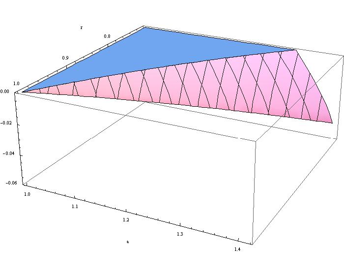
Figure 11.2: $h((1-ar)/2)/4+\log(\frac{1+r}{2})\log(4/3)/2$, where we only show the region below 0, i.e., where security can be attained.

11.6 Conclusion

We have introduced the model of noisy-quantum storage. In this model, we have determined security bounds for a perfect ROT protocol given collective storage attacks by Bob. Furthermore, we showed how to construct a practical ROT where we do allow the honest parties to experience noise during transmissions and their operations as well. We provided an explicit security tradeoff between the noise affecting the honest parties, and the noise during storage for a dishonest Bob.

Ideally, we would like to show security against general coherent noisy attacks. The problem with analyzing a coherent attack of Bob described by some super-operator ${\cal S}$ affecting all his incoming qubits is not merely a technical one: one first needs to determine a realistic noise model in this setting. It may be possible using variations of de Finetti theorems as in the proof of QKD [Ren05] to prove for a symmetrized version of our protocol that any coherent attack by Bob is equivalent to a collective attack. Yet, the present scenario differs in that it is not as straightforward to achieve a symmetrization of the protocol. However, one can in fact analyze a specific type of coherent noise, one that essentially corresponds to an eavesdropping attack in QKD. Note that the 1-2 OT protocol can be seen as two runs of QKD interleaved with each other. The strings $f(x_{|\mathcal{I}_{+}})$ and $f(x_{|\mathcal{I}_{\times}})$ are then the two keys generated. The noise must be such that it leaves Bob with exactly the same information as the eavesdropper Eve in QKD. In this case, it follows from the security of QKD that the dishonest Bob (learning exactly the same information as the eavesdropper Eve) does not learn anything about the two keys.

In terms of long-term security, fault-tolerant photonic computation (e.g., with the KLM scheme [KLM01]) might allow a dishonest Bob to encode the incoming quantum information into a fault-tolerant quantum memory. This implies that in storage, the effective noise rate can be made arbitrarily small. However, the encoding of a single unknown state is not a fault-tolerant quantum operation: already the encoding process introduces errors whose rates cannot be made arbitrarily small with increasing effort. Hence, even in the presence of a quantum computer, there is a residual storage noise rate due to the unprotected encoding operations. The question of security then becomes a question of a trade-off between this residual noise rate versus the intrinsic noise rate. Finally, it remains to address composability of the protocol within our model, which has already been considered for the bounded-quantum-storage model [WW07].

Appendix A Linear algebra and semidefinite programming

Semidefinite programming is a useful tool to solve optimization problems. Since we employed semidefinite programming in Chapters 3, 7, and 11, we briefly state the most important notions. We refer to [BV04] for an in-depth introduction.

A.1 Linear algebra prerequisites

Before turning to semidefinite programming in the next section, we first briefly recall some elementary definitions from linear algebra. We thereby assume the reader is familiar with basic concepts, such as matrix multiplication and addition. Unless explicitly indicated, all vector spaces $V$ considered here are over the field of complex numbers. We use $V=\mathbb{C}^{d}$ to denote a $d$-dimensional complex vector space, and $\mathbb{C}^{d\times d}$ to denote the space of complex $d\times d$ matrices. A set of vectors $|v_{1}\rangle,\ldots,|v_{d}\rangle\in V$ is linearly independent if $\sum_{i=1}^{d}a_{i}|v_{i}\rangle=0$ implies that $a_{1}=\ldots=a_{d}=0$. A basis of a $d$-dimensional vector space $V$ is a set of linearly independent vectors $|v_{1}\rangle,\ldots,|v_{d}\rangle\in V$, the basis vectors, such that any vector $|u\rangle\in V$ can be written as a linear combination of basis vectors. If there exists a vector $|v\rangle\in V$ with $|v\rangle\neq 0$ such that $A|v\rangle=\lambda|v\rangle$, we say that $|v\rangle$ is an eigenvector of $A$ and the scalar $\lambda$ the corresponding eigenvalue.

The inner product of two vectors $|u\rangle,|v\rangle\in V$ with $|u\rangle=(u_{1},\ldots,u_{d})$ and $|v\rangle=(v_{1},\ldots,v_{d})$ is given by $\langle{u}|{v}\rangle=\sum_{i}u_{i}^{*}v_{i}$. The 2-norm of a vector is given by $|||v\rangle||=\sqrt{\langle{v}|{v}\rangle}$. Unless otherwise indicated, all norms of a vector are 2-norms in this text. We also use $|||v\rangle||_{V}$ to denote emphasize that the norm is defined on a vector space $V$. Two vectors $|u\rangle,|v\rangle\in V$ such that $\langle{u}|{v}\rangle=0$ are orthogonal. If, in addition, $|||u\rangle||=|||v\rangle||=1$ then they are also called orthonormal.

A Hilbert space is defined as a vector space $V$ with an inner product, where the vector space is complete. We refer to [Con90] for a formal definition of the notion of completeness and merely note that informally a vector space is complete if for any sequence of vectors in said space approaching a limit, the limit is also an element of the vector space. A bounded operator is an operator $A:V\rightarrow V^{\prime}$ such that there exists a $c\in\mathbb{R}$ satisfying $||A|v\rangle||_{V^{\prime}}\leq c|||v\rangle||_{V}$ for all $v\in V$. The smallest such $c$ is also called the operator norm of $A$.

The transpose of a matrix $A$ is written as $A^{T}$ and given by $A^{T}_{ij}=A_{ji}$, where $A_{ij}$ denotes the entry of the matrix $A$ at column $i$ and row $j$. Similarly, the conjugate transpose $A^{\dagger}$ of $A$ is of the form $A^{\dagger}_{ij}=A_{ji}^{*}$. We use $\mathbb{I}$ to denote the identity matrix defined as $\mathbb{I}=[\mathbb{I}_{ij}]$ with $\mathbb{I}_{ij}=\delta_{ij}$. A matrix $U$ is called unitary if $UU^{\dagger}=U^{\dagger}U=\mathbb{I}$. Furthermore, $M$ is called Hermitian if and only if $M=M^{\dagger}$. Any Hermitian matrix can be decomposed in terms of its eigenvalues $\lambda_{j}$ and eigenvectors $|u_{j}\rangle$ as $M=\sum_{j}\lambda_{j}|u_{j}\rangle\langle u_{j}|$, where $|u_{j}\rangle\langle u_{j}|$ is a projector onto the vector $|u_{j}\rangle$. We also call this the eigendecomposition of $M$. The support of $M$ is the space spanned by all its eigenvectors with non-zero eigenvalue.

The tensor product of an $m\times n$-matrix $A$ and an $m^{\prime}\times n^{\prime}$ matrix $B$ is given by the $mm^{\prime}\times nn^{\prime}$-matrix

$$A\otimes B=\left(\begin{array}[]{ccc}A_{11}B&\ldots&A_{1n}B\\ A_{21}B&\ldots&A_{2n}B\\ &\ddots&\\ A_{n1}B&\ldots&A_{nn}B\\ \end{array}\right).$$

The tensor product is also defined for two vector spaces $V$ and $V^{\prime}$. In particular, if the basis of the $d$-dimensional vector space $V$ is given by $\{|v_{1}\rangle,\ldots,|v_{d}\rangle\}$ and the basis of the $d^{\prime}$-dimensional vector space $V^{\prime}$ is given by $\{|v^{\prime}_{1}\rangle,\ldots,|v^{\prime}_{d^{\prime}}\rangle\}$, then $W=V\otimes V^{\prime}$ denotes the $d\cdot d^{\prime}$-dimensional vector space $W$ with basis $\{|v_{i}\rangle\otimes|v^{\prime}_{j}\rangle\mid i\in[d],j\in[d^{\prime}]\}$.

The direct sum of an $m\times n$-matrix $A$ and an $m^{\prime}\times n^{\prime}$ matrix $B$ is given by the $m+m^{\prime}\times n+n^{\prime}$ matrix

$$\left(\begin{array}[]{cc}A&0\\ 0&B\end{array}\right).$$

Two vector spaces $V$ and $V^{\prime}$ defined as above can also be composed in an analogous fashion yielding a $d+d^{\prime}$ dimensional vector space $W=V\oplus V^{\prime}$, where any $|w\rangle\in W$ can be written as $|w\rangle=|v\rangle\oplus|v^{\prime}\rangle$ for some $|v\rangle\in V$ and $|v^{\prime}\rangle\in V^{\prime}$ with $|v\rangle\oplus|v^{\prime}\rangle=(v_{1},\ldots,v_{d},v^{\prime}_{1},\ldots,v^{\prime}_{d^{\prime}})$ for $|v\rangle=(v_{1},\ldots,v_{d})$ and $|v^{\prime}\rangle=(v^{\prime}_{1},\ldots,v^{\prime}_{d^{\prime}})$.

The trace of a matrix $A$ is given by the sum of its diagonal entries $\mbox{\rm Tr}(A)=\sum_{i}A_{ii}$. Note that $\mbox{\rm Tr}(A+B)=\mbox{\rm Tr}(A)+\mbox{\rm Tr}(B)$, and $\mbox{\rm Tr}(AB)=\mbox{\rm Tr}(BA)$. If $A$ is an Hermitian matrix, then $\mbox{\rm Tr}(A)$ is the sum of its eigenvalues.

Finally, the rank of a matrix $A$ is denoted as $\mbox{rank}(A)$ and given by the maximal number of linearly independent columns (or rows) of $A$.

A.2 Definitions

We now turn to the definitions relevant for our discussion of semidefinite programming. A Hermitian matrix $M$ is positive semidefinite if and only if all of its eigenvalues are non-negative [HJ85, Theorem 7.2.1]. Throughout this text, we use $M\geq 0$ to indicate that $M$ is positive semidefinite. We know from [HJ85, Theorem 7.2.11]:

Proposition A.2.1.

For a Hermitian matrix $M\in\mathbb{C}^{d\times d}$ the following three statements are equivalent:

1. $M\geq 0$,

2. $x^{\dagger}Mx\geq 0$ for all vectors $x\in\mathbb{C}^{d}$,

3. $M=G^{\dagger}G$ for some matrix $G\in\mathbb{C}^{d\times d}$.

$M$ is called positive definite if and only if all of its eigenvalues are positive: we have $x^{\dagger}Mx>0$ for all vectors $x\in\mathbb{C}^{d}$. We use $M>0$ to indicate that $M$ is positive definite. We also encounter projectors, where a Hermitian matrix $M$ is a projector if and only if $M^{2}=M$. Note that this implies that $M\geq 0$. We say that two projectors $M_{1}$ and $M_{2}$ are orthogonal projectors if and only if $M_{1}M_{2}=0$.

Furthermore, we use $\mathcal{S}^{d}$ to denote the set of all Hermitian matrices, $\mathcal{S}^{d}=\{X\in\mathbb{C}^{d\times d}\mid X=X^{\dagger}\}$, and $\mathcal{S}^{d}_{+}=\{X\in\mathcal{S}^{d}\mid X\geq 0\}$ for the set of all positive semidefinite matrices. A set $\mathcal{T}$ is a cone, if for any $\alpha\geq 0$ and $T\in\mathcal{T}$ we have $\alpha T\in\mathcal{T}$. A set $\mathcal{T}$ is convex, if for any $\alpha\in[0,1]$ and $T_{1},T_{2}\in\mathcal{T}$ we have $\alpha T_{1}+(1-\alpha)T_{2}\in\mathcal{T}$. A set $\mathcal{T}$ is called a convex cone, if $\mathcal{T}$ is convex and a cone: for any $\alpha_{1},\alpha_{2}\geq 0$ and $T_{1},T_{2}\in\mathcal{T}$ we must have that $\alpha_{1}T_{1}+\alpha_{2}T_{2}\in\mathcal{T}$. Note that $\mathcal{S}^{d}_{+}$ is a convex cone: Let $\alpha_{1},\alpha_{2}\geq 0$, and $A,B\in\mathcal{S}^{d}_{+}$. Then for any $x\in\mathbb{C}^{d}$ we have

$$x^{\dagger}(\alpha_{1}A+\alpha_{2}B)x=\alpha_{1}x^{\dagger}Ax+\alpha_{2}x^{\dagger}Bx\geq 0.$$

Hence, $\alpha_{1}A+\alpha_{2}B\in\mathcal{S}^{d}_{+}$. The following will be of use in Chapter 3.

Proposition A.2.2.

Let $A,B\in S^{d}$. Then $A\geq 0$ if and only if for all $B\geq 0$ $\mbox{\rm Tr}(AB)\geq 0$.

Proof A.2.3.

Suppose that $A\geq 0$. Note that we can decompose $B=\sum_{j}\lambda_{j}|u_{j}\rangle\langle u_{j}|$ where for all $j$ $\lambda_{j}\geq 0$ since $B\geq 0$. Hence, $\mbox{\rm Tr}(AB)=\sum_{j}\lambda_{j}\mbox{\rm Tr}(A|u_{j}\rangle\langle u_{j}|)=\sum_{j}\lambda_{j}\langle u_{j}|A|u_{j}\rangle\geq 0$, since $A\geq 0$.

To prove the converse, suppose on the contrary that for all $B\geq 0$ we have $\mbox{\rm Tr}(AB)\geq 0$, but $A\not\geq 0$. If $A\not\geq 0$, then there exists some vector $|v\rangle$ such that $\langle v|A|v\rangle<0$. Let $B=|v\rangle\langle v|$. Clearly, $B\geq 0$ and $\mbox{\rm Tr}(AB)=\langle v|A|v\rangle<0$ which is a contradiction.

A.3 Semidefinite programming

Semidefinite programming is a special case of convex optimization. Its goal is to solve the following semidefinite program (SDP) in terms of the variable $M\in\mathcal{S}^{d}$

maximize	$\mbox{\rm Tr}(CM)$
subject to	$\mbox{\rm Tr}(A_{i}M)=b_{i},i=1,\ldots,p$, and $M\geq 0$

for given matrices $C,A_{1},\ldots,A_{p}\in\mathcal{S}^{d}$. The above form is called the standard form of an SDP, and any SDP can be cast in this fashion (possibly at the expense of additional variables) [BV04]. To gain some geometric intuition about this task, note that $M\geq 0$ means that $M$ must lie in the cone $\mathcal{S}^{d}_{+}$. The constraints $Tr(A_{i}M)=b_{i}$ determine a set of hyperplanes which further limit our possible solutions. A matrix $M$ is called feasible, if it satisfies all constraints.

An important aspect of semidefinite programming is duality. Intuitively, the idea behind Lagrangian duality is to extend the objective function (here $\mbox{\rm Tr}(CM)$) with a weighted sum of the constraints in such a way, that we will be penalized if the constraints are not fulfilled. The weights then correspond to the dual variables. Optimizing over these weights then gives rise to the dual problem. The original problem is called the primal problem. For the above SDP in standard form, we can write down the Lagrangian as

$$L(M,\lambda_{1},\ldots,\lambda_{p},K) = \mbox{\rm Tr}(CM)+\sum_{i=1}^{p}\lambda_{i}(b_{i}-\mbox{\rm Tr}(A_{i}M))+\mbox{\rm Tr}(KM)$$

$$= \mbox{\rm Tr}((C-\sum_{i}\lambda_{i}A_{i}+K)M)+\sum_{i}\lambda_{i}b_{i},$$

where $K\geq 0$. The dual function is then

$$g(\lambda_{1},\ldots,\lambda_{p},K) = \sup_{M}\left(\mbox{\rm Tr}((C-\sum_{i}\lambda_{i}A_{i}+K)M)+\sum_{i}\lambda_{i}b_{i}\right)$$

$$= \left\{\begin{array}[]{ll}\sum_{i}\lambda_{i}b_{i}&\mbox{if }C-\sum_{i}\lambda_{i}A_{i}+K=0\\[1.42262pt] \infty&\mbox{otherwise}\end{array}\right.$$

From $C-\sum_{i}\lambda_{i}A_{i}+K=0$ and $K\geq 0$, we obtain that $K=-C+\sum_{i}\lambda_{i}A_{i}\geq 0$. This gives us the dual problem as

minimize	$\sum_{i}\lambda_{i}b_{i}$
subject to	$\sum_{i}\lambda_{i}A_{i}\geq C$,

where the optimization is now over the dual variables $\lambda_{i}$.

We generally use $d^{*}$ to denote the optimal value of the dual problem, and $p^{*}$ for the optimal value of the primal problem. Weak duality says that $d^{*}\geq p^{*}$. Let’s see why this is true in the above construction of the dual problem. Let $M^{(*)}$ and $\{\lambda_{i}^{(*)}\}$ be the optimal solutions to the primal and dual problem respectively. In particular, this means that $M^{(*)}$ and $\{\lambda_{i}^{(*)}\}$ must satisfy the constraints. Then

$$d^{*}-p^{*} = \sum_{i}\lambda_{i}^{(*)}b_{i}-\mbox{\rm Tr}(CM^{(*)})$$

$$= \sum_{i}\lambda_{i}^{(*)}\mbox{\rm Tr}(A_{i}M^{(*)})-\mbox{\rm Tr}(CM^{(*)})$$

$$= \mbox{\rm Tr}\left(\left(-C+\sum_{i}\lambda_{i}^{(*)}A_{i}\right)M^{(*)}\right)\geq 0,$$

by Proposition A.2.2 since $M^{(*)}\geq 0$ and $\sum_{i}\lambda_{i}^{(*)}A_{i}\geq C$. An important consequence of weak duality, is that if we have $d^{*}=p^{*}$ for a feasible dual and primal solution respectively, we can conclude that both solutions are optimal. If solutions exist such that $d^{*}=p^{*}$, we also speak of strong duality. We know from Slater’s conditions [BV04], that strong duality holds if there exists a feasible solution to the primal problem which also satisfies $M>0$.

A.4 Applications

In many quantum problems, we want to optimize over states, or measurement operators. Evidently, semidefinite programming is very well suited to this case: When optimizing over a state $\rho$, we ask that $\rho\geq 0$ and $\mbox{\rm Tr}(\rho)=1$. When optimizing over measurement operators $M_{1},\ldots,M_{k}$ belonging to one POVM, we ask that $M_{j}\geq 0$ for all $j\in[k]$ and $\sum_{j}M_{j}=\mathbb{I}$. Concrete examples can be found in Chapters 3, 7, and 11.

Appendix B $C^{*}$-Algebra

As $C^{*}$-algebras are not usually encountered in computer science, we briefly state the most important results we will refer to for convenience. In particular, they help us understand the framework of post-measurement information we encountered in Chapter 3 as well as the structure of bipartite non-local games in Chapter 6.

B.1 Introduction

Instead of starting out with the usual axioms of quantum states and their evolutions, any physical system can be characterized by a $C^{*}$-algebra $\mathscr{A}$ of observables. States of this system are now identified purely by means of measurements of these observables. This starting point is rather beautiful in its abstraction: So far, nothing has been said how we can represent elements of this algebra. Yet, it turns out that all the usual axioms can be derived from this abstract structure: we can represent observables as operators and states as vectors in a Hilbert space. In fact, any such algebra $\mathscr{A}$ is isomorphic to an algebra of bounded operators on a Hilbert space. So why should we bother adopting this abstract viewpoint? It turns out that $C^{*}$-algebras often make it easier to understand the fundamental differences between the classical and the quantum setting. If the algebra $\mathscr{A}$ is abelian, we have a classical system. Otherwise, our system is inherently quantum. Commutativity leads to several nice structural properties of an algebra which have been exploited to answer many central questions in quantum information: When can we clone physical states? What information can be extracted without disturbing the system? That is, what part of a system is in fact classical and what is truly quantum?

Here, we will mere scratch the surface of this formalism. In particular, we will focus on finite-dimensional $C^{*}$-algebras only, which is all we will need in Chapters 3 and 6. For more information, consult any textbook on the topic [Tak79, BR02, Arv76]. We assume that the reader is familiar with the basic concepts such as a Hilbert space and refer to [Con90] for an introduction. First, we need to introduce some essential definitions in Section B.2. We then examine states and observables, and their familiar representation in a Hilbert space in Section B.3.2. In Section B.4, we then concentrate on commutation: We will sketch how from commutation relations we in fact obtain a bipartite structure. It turns out that commutation relations also play an important role in determining which operations leave states invariant. Looking at the structure of the problem, it turns out that in fact many problems ranging from cloning to post-measurement information and bipartite non-local games are quite closely related.

B.2 Some terminology

A Banach algebra $\mathscr{A}$ is a linear associative algebra which is also a Banach space, with the property that for all $A$ and $B\in\mathscr{A}$ we have

$$\mbox{$\parallel{AB}\parallel$}\leq\mbox{$\parallel{A}\parallel$}\mbox{$\parallel{B}\parallel$}.$$

The norm $\parallel{A}\parallel$ of $A$ is thereby a real number satisfying the usual requirements that for all $A\in\mathscr{A}$ we have $\mbox{$\parallel{A}\parallel$}\geq 0$ where $\mbox{$\parallel{A}\parallel$}=0$ if and only if $A=0$, $\mbox{$\parallel{\alpha A}\parallel$}=\alpha\mbox{$\parallel{A}\parallel$}$, $\mbox{$\parallel{A+B}\parallel$}\leq\mbox{$\parallel{A}\parallel$}+\mbox{$\parallel{B}\parallel$}$, and $\mbox{$\parallel{AB}\parallel$}\leq\mbox{$\parallel{A}\parallel$}\mbox{$\parallel{B}\parallel$}$. $\mathscr{A}$ is called a $*$-algebra if it has the additional property that it admits an involution $A\rightarrow A^{\dagger}\in\mathscr{A}$ such that for all $A$ and $B\in\mathscr{A}$ the following holds: $(A^{\dagger})^{\dagger}=A$, $(A+B)^{\dagger}=A^{\dagger}+B^{\dagger}$, $(\alpha A)^{\dagger}=\bar{\alpha}A^{\dagger}$, and $(AB)^{\dagger}=B^{\dagger}A^{\dagger}$. A $C^{*}$-algebra is now an even more special case: in addition we also have that $\mbox{$\parallel{A^{\dagger}A}\parallel$}=\mbox{$\parallel{A}\parallel$}^{2}$ for all $A\in\mathscr{A}$. This also gives us $\mbox{$\parallel{A^{\dagger}}\parallel$}=\mbox{$\parallel{A}\parallel$}$. In the following we will simply use the term “algebra” to refer to a $C^{*}$-algebra. The trick is not to be intimidated. It is easier to have a more concrete picture in mind: For example, the algebra $\mathbb{B}(\mathcal{H})$ of all bounded operators on a Hilbert space $\mathcal{H}$ is a $C^{*}$-algebra, when we take sums and products of operators in the usual way and take our norm to be the operator norm $\mbox{$\parallel{A}\parallel$}=\sup(\mbox{$\parallel{Av}\parallel$}\mid v\in\mathcal{H},\mbox{$\parallel{v}\parallel$}=1)$, where $\mbox{$\parallel{v}\parallel$}^{2}=\langle{v}|{v}\rangle$ for the inner product $\langle{\cdot}|{\cdot}\rangle$ of the Hilbert space. This algebra is closed under all the usual operations such as addition, multiplication, and multiplication by scalars and the involution operation. This involution is now the adjoint operation $A\rightarrow A^{\dagger}$, which in physics is usually denoted by $\dagger$ instead of $*$. In some physics papers, you will therefore also find the name $\dagger$-algebra instead. As in the example of post-measurement information, we are also often interested in the $*$-algebra generated by a given set of operators. Any operator $X$ in a Hilbert space $\mathcal{H}$ determines a $C^{*}$-algebra $\mathscr{A}$ which we will denote by $\mathscr{A}=\langle X\rangle$. This is the smallest $C^{*}$-algebra which contains both $X$ and the identity, i.e. $\langle X\rangle=\bigcap_{X,\mathbb{I}\in\mathscr{B}}\mathscr{B}$. What’s included in $\langle X\rangle$? Recall that $\mathscr{A}$ is closed under the adjoint operation so we definitely have $X^{\dagger}$. In addition, our conditions above imply that we will see all possible polynomials in $X$ and $X^{\dagger}$. For example, $X+X^{\dagger}$ and $XX^{\dagger}$ are also elements of the algebra. We use $\langle X_{1},\ldots,X_{k}\rangle$ to denote the $C^{*}$-algebra generated by operators $X_{1},\ldots,X_{k}$, and $\langle\mathcal{S}\rangle$ to denote the algebra generated by operators from the set $\mathcal{S}$.

If an algebra $\mathscr{B}$ satisfies $\mathscr{B}\subseteq\mathscr{A}$, we call $\mathscr{B}$ a subalgebra of $\mathscr{A}$. An algebra $\mathscr{A}$ is unital if it contains the identity. We will always use $\mathbb{I}$ to denote the identity element. Since we restrict ourselves to the finite-dimensional case, we can assume that any $C^{*}$-algebra is in fact unital [Tak79]. We will always take $\mathscr{A}$ to be unital here. An element $A\in\mathscr{A}$ of a Banach algebra $\mathscr{A}$ is called invertible if there exists some $A^{\prime}\in\mathscr{A}$ such that $AA^{\prime}=A^{\prime}A=\mathbb{I}$. Furthermore, for a $C^{*}$-algebra $\mathscr{A}$, the spectrum of $A\in\mathscr{A}$ is given by $\mbox{Sp}_{\mathscr{A}}(A)=\{\lambda\in\mathbb{C}\mid A-\lambda\mathbb{I}\mbox{ is not invertible}\}$. Note that for any $A\in\mathbb{B}(\mathcal{H})$, this is just the spectrum of the operator relative to $\mathbb{B}(\mathcal{H})$ in the usual sense.

A left ideal in some algebra $\mathscr{A}$ is a subalgebra $\mathscr{B}\subseteq\mathscr{A}$ such that for any elements $B\in\mathscr{B}$ and $A\in\mathscr{A}$ we have that $AB\in\mathscr{B}$. Similarly, $\mathscr{B}$ is called a right ideal if $BA\in\mathscr{B}$. A two-sided ideal or simply ideal has both properties: $\mathscr{B}$ is both a left and right ideal of $\mathscr{A}$. An algebra $\mathscr{A}$ is called simple if its only ideals are $\{0\}$ and $\mathscr{A}$ itself. An algebra $\mathscr{A}$ is called semisimple, if it can be written as the direct sum of simple algebras. To get a better feeling for what this actually means, it is perhaps again helpful to think of a particular representation of the algebra in terms of bounded operators on a Hilbert space. In terms of representations, being simple means that the representation is irreducible. Being semisimple then means that the representation is completely reducible: i.e. for the representation $\pi$ of $A$ we can express $\pi(A)$ as a sum of irreducible representations. We will examine this decomposition in more detail in Section B.4.1.

B.3 Observables, states and representations

B.3.1 Observables and states

A physical system is characterized by a set of measurable quantities, i.e. observables. As mentioned above, we will assume that a physical system is in fact described by a $C^{*}$-algebra $\mathscr{A}$ of observables. As we will see below, we can take the observables to live in a Hilbert space $\mathcal{H}$, and $\mathscr{A}\subseteq\mathbb{B}(\mathcal{H})$. Where do the states come in? In the language of $C^{*}$-algebras, states are positive linear functionals on $\mathscr{A}$: A linear functional on an algebra is a function $f:\mathscr{A}\rightarrow\mathbb{C}$ such that for all $A,B\in\mathscr{A}$ we have $f(A+B)=f(A)+f(B)$ and $f(\alpha A)=\alpha f(A)$ where $\alpha\in\mathbb{C}$ is a scalar. A linear functional is called positive if $f(A)\geq 0$ for any $A\in\mathscr{A}$ whenever $A\geq 0$. A state on $\mathscr{A}$ is a positive linear functional $f$ on $\mathscr{A}$ with the additional property that it has norm 1, i.e., $f(\mathbb{I})=1$. The set of states is a convex set of linear functionals and its extreme elements are called pure states. The set of all states on an algebra $\mathscr{A}$ is also called the state space, often denoted by $\mathcal{E}(\mathscr{A})$. Any observable $A\in\mathscr{A}$ in our algebra is uniquely characterized by the expectation of all states when we measure $A$: So the value of $f(A)$ for all states $f\in\mathcal{E}(\mathscr{A})$ in our state space uniquely characterizes any element $A$ of our algebra. The converse is also true: the value of $f(A)$ for all $A\in\mathscr{A}$ completely characterizes the state $f$. To get a better feeling for this, it is again helpful to think of an algebra $\mathscr{A}\subseteq\mathbb{B}(\mathcal{H})$. Given a vector $v$ living in the Hilbert space $\mathcal{H}$, we can construct a linear functional on $\mathscr{A}$ by letting $f(A)=\langle{v}|{Av}\rangle$. The same is true if we consider any abstract $\mathscr{A}$ and its representation $\pi$ on a Hilbert space, by letting $f(A)=\langle{v}|{\pi(A)v}\rangle$ given $v\in\mathcal{H}$.

B.3.2 Representations

We now examine how an abstract $C^{*}$-algebra can be represented by a set of operators on a Hilbert space, via the famous construction by Gelfand, Naimark and Segal. An account of this construction can be found in any standard textbook on $C^{*}$-algebra [Tak79, BR02, Arv76]. For completeness, we here give a heavily annotated, largely self-contained, explanation of the GNS construction. As it turns out, by the GNS construction, any $C^{*}$-algebra is isomorphic to an algebra of bounded operators, a result which we will merely state here. When trying to find a representation of a $C^{*}$-algebra $\mathscr{A}$, our goal is to find a pair $(\pi,\mathcal{H})$ where $\mathcal{H}$ is a Hilbert space and $\pi:\mathscr{A}\rightarrow\mathscr{B}(\mathcal{H})$ is a $*$-homomorphism which maps any element of our algebra to a bounded operator in the chosen Hilbert space.

Theorem B.3.1 (GNS).

Let $\mathscr{A}$ be a unital $C^{*}$-algebra, and let $f$ be a positive linear functional on $\mathscr{A}$. Then there exists a representation $(\mathcal{H}_{f},\pi_{f})$ of $\mathscr{A}$ with a Hilbert space $\mathcal{H}_{f}$, a $*$-homomorphism $\pi_{f}:\mathscr{A}\rightarrow\mathbb{B}(\mathcal{H}_{f})$ and a vector $\Phi_{f}\in\mathcal{H}_{f}$ such that for all $A\in\mathscr{A}$

$$f(A)=\langle{\Phi_{f}}|{\pi_{f}(A)\Phi_{f}}\rangle.$$

Proof B.3.2.

First, we construct the Hilbert space $\mathcal{H}_{f}$. Since $\mathscr{A}$ is a Banach space, we can turn it into a pre-Hilbert space by defining the positive semidefinite sesquilinear form

$$\langle{A}|{B}\rangle_{f}=f(A^{\dagger}B),$$

for all $A,B\in\mathscr{A}$. Note that this form may be degenerate. In order to eliminate this degeneracy, consider

$$\mathcal{I}_{f}=\{A\mid A\in\mathscr{A}\mbox{ and }f(A^{\dagger}A)=0\}.$$

Note that $\mathcal{I}_{f}$ is a linear subspace of $\mathscr{A}$ since for all $I,J\in\mathcal{I}_{f}$ we have $f((I+J)^{\dagger}(I+J))=f(I^{\dagger}I)+f(J^{\dagger}I)+f(I^{\dagger}J)+f(J^{\dagger}J)\leq 2\sqrt{f(J^{\dagger}J)f(I^{\dagger}I)}=0$, where we used the Cauchy-Schwarz inequality.

We now show that $\mathcal{I}_{f}$ is a left ideal of $\mathscr{A}$: Let $I\in\mathcal{I}_{f}$ and $A,B\in\mathscr{A}$. We then need to show that $AI\in\mathcal{I}_{f}$. Indeed, from $(AI)^{\dagger}(AI)\geq 0$ we have

$$0\leq f((AI)^{\dagger}(AI))=f(I^{\dagger}A^{\dagger}AI)\leq\sqrt{f(I^{\dagger}I)f((A^{\dagger}AI)^{\dagger}(A^{\dagger}AI))}=0,$$

where the inequality follows from the Cauchy-Schwarz inequality.

The Hilbert space $\mathcal{H}_{f}$ is then constructed by completing the quotient space $\mathscr{A}/\mathcal{I}_{f}$. This works as follows: Define the equivalence classes

$$\Psi_{A}=\{A+I\mid I\in\mathcal{I}_{f}\}.$$

Note that these equivalence classes constitute a complex vector space on their own, where addition and scalar multiplication are defined via the following operations inherited from $\mathscr{A}$. We have $\Psi_{A+B}=\Psi_{A}+\Psi_{B}$ and $\Psi_{\alpha A}=\alpha\Psi_{A}$. We can then define the inner product

$$\langle{\Psi_{A}}|{\Psi_{B}}\rangle=\langle{A}|{B}\rangle_{f}=f(A^{\dagger}B).$$

Note that $\Psi_{A}$ and $\Psi_{B}$ of course depend on $f$. One can verify that this a correct definition. Indeed, the inner product does not depend on our choice of representative from each equivalence class: Let $I_{1},I_{2}\in\mathcal{I}_{f}$, and let $A,B\in\mathscr{A}$. Then

$$f((A+I_{1})^{\dagger}(B+I_{2}))=f(A^{\dagger}B)+f(A^{\dagger}I_{2})+f(I_{1}^{\dagger}B)+f(I_{1}^{\dagger}I_{2})=f(A^{\dagger}B),$$

where the last equality follows again from the Cauchy-Schwarz inequality. We can now obtain $\mathcal{H}_{f}$ by forming the completion of this space. It is well-known in functional analysis that any strict pre-Hilbert space can be embedded as a dense subspace of a Hilbert space in such a way that the inner product is preserved.

Second, we must construct $\pi_{f}$. We first define the action of $\pi_{f}(A)$ on the vectors constructed above as

$$\pi_{f}(A)\Psi_{B}=\Psi_{AB}.$$

Note that this definition is again independent of our choice of representative from each equivalence class since for all $A,B\in\mathscr{A}$ we have

$$\pi_{f}(A)\Psi_{B+I}=\Psi_{A(B+I)}=\Psi_{AB+AI}=\Psi_{AB}=\pi_{f}(A)\Psi_{B},$$

since $\mathcal{I}_{f}$ is a left ideal of $\mathscr{A}$ and we already saw that $AI\in\mathcal{I}_{f}$. It remains to show that $\pi_{f}$ is a homomorphism and that $\pi_{f}(A)$ is indeed bounded. To see that $\pi_{f}$ is a homomorphism, note that

$$\pi_{f}(AB)\Psi_{C}=\Psi_{ABC}=\pi_{f}(A)\pi_{f}(B)\Psi_{C}$$

and

$$\pi_{f}(\lambda A+\gamma B)\Psi_{C}=\Psi_{\lambda A+\gamma B}=\lambda\Psi_{A}+\gamma\Psi_{B}=(\lambda\pi_{f}(A)+\gamma\pi_{f}(B))\Psi_{C},$$

as desired. To see that $\pi_{f}(A)$ is bounded, consider

$$\mbox{$\parallel{\pi_{f}(A)\Psi_{B}}\parallel$}^{2} = \langle{\Psi_{AB}}|{\Psi_{AB}}\rangle=f((AB)^{\dagger}(AB))$$

$$= f(B^{\dagger}A^{\dagger}AB)\leq\mbox{$\parallel{A}\parallel$}^{2}f(B^{\dagger}B)\leq\mbox{$\parallel{A}\parallel$}^{2}\mbox{$\parallel{\Psi_{B}}\parallel$}^{2},$$

where we used the fact that from $B^{\dagger}A^{\dagger}AB\leq\mbox{$\parallel{A}\parallel$}^{2}B^{\dagger}B$ we have $f(B^{\dagger}A^{\dagger}AB)\leq\mbox{$\parallel{A}\parallel$}^{2}f(B^{\dagger}B)$ (see for example [Tak79]).

Finally, we need to construct the vector $\Phi_{f}$. Since $\mathscr{A}$ is unital we can take $\Phi_{f}=\Psi_{\mathbb{I}}$. This gives us $\langle{\Phi_{f}}|{\pi_{f}(A)\Phi_{f}}\rangle=\langle{\Psi_{\mathbb{I}}}|{\pi_{f}(A)\Psi_{\mathbb{I}}}\rangle=\langle{\Psi_{\mathbb{I}}}|{\Psi_{A}}\rangle=f(\mathbb{I}^{\dagger}A)=f(A)$. Note that $\pi_{f}(A)\Psi_{\mathbb{I}}=\Psi_{A}$, i.e., $\Phi_{f}=\Psi_{\mathbb{I}}$ is cyclic for $(\mathcal{H}_{f},\pi_{f})$.

The resulting representation is irreducible if and only if $f$ is pure [BR02, Theorem 2.3.19]. By considering a family of states $F$, and applying the GNS construction to all $f\in F$ and taking the direct sum of representations it is then possible to show that:

Theorem B.3.3.

(GN) Let $\mathscr{A}$ be a unital $C^{*}$-algebra. Then $\mathscr{A}$ is isomorphic to an algebra of bounded operators on a Hilbert space $\mathcal{H}$.

B.4 Commuting operators

$\mathscr{A}$ is abelian if and only if the physical system corresponding to this algebra is classical. Thus to distinguish the quantum from the classical problems, commutation will be central to our discussion. In fact, it leads to very nice structural properties which we already exploited in Chapter 3. First, however, we will need a bit more terminology. The commutator of two operators $A$ and $B$ is given by $[A,B]=AB-BA$. For quantum applications, two observables $A$ and $B$ are called compatible if they commute, i.e., $[A,B]=0$. Conversely, $A$ and $B$ are called complementary if $[A,B]\neq 0$. The center $\mathscr{Z}_{\mathscr{A}}$ of an algebra $\mathscr{A}$ is the set of all elements in $\mathscr{A}$ that commute with all elements of $\mathscr{A}$, i.e.

$$\mathscr{Z}_{\mathscr{A}}=\{Z\mid Z\in\mathscr{A},\forall A\in\mathscr{A}:[Z,A]=0\}.$$

It is easy to see that if $\mathscr{A}$ only has a trivial center, i.e. $\mathscr{Z}_{\mathscr{A}}=\{c\mathbb{I}\mid c\in\mathbb{C}\}$, $\mathscr{A}$ is simple [Tak79]. If $\mathscr{A}\subseteq\mathbb{B}(\mathcal{H})$ for some Hilbert space $\mathcal{H}$, then the commutant of $\mathscr{A}$ in $\mathbb{B}(\mathcal{H})$ is

$$\mbox{Comm}(\mathscr{A})=\{X\mid X\in\mathbb{B}(\mathcal{H}),\forall A\in\mathscr{A}:[X,A]=0\}.$$

We have $\mathscr{Z}_{\mathscr{A}}=\mathscr{A}\cap\mbox{Comm}(\mathscr{A})$.

B.4.1 Decompositions

In any of our problems, the interesting case is when the algebra $\mathscr{A}$ under consideration is in fact simple: that is, “fully quantum”. In all problems we will consider, it will turn out that we can always break down the problem into smaller components by decomposing any $\mathscr{A}$ into a sum of simple algebras. Luckily, such a decomposition always exists in the finite-dimensional case:

Lemma B.4.1.

Let $\mathscr{A}$ be a finite-dimensional $C^{*}$-algebra. Then there exists a decomposition

$$\mathscr{A}=\bigoplus_{j}\mathscr{A}_{j},$$

such that $\mathscr{A}_{j}$ is simple.

Proof B.4.2.

Let $\mathscr{Z}_{A}$ be the center of $\mathscr{A}$. Clearly, since $\mathscr{A}$ is finite-dimensional, $\mathscr{Z}_{A}$ is a finite-dimensional abelian $C^{*}$-algebra. Since $\mathscr{Z}_{A}$ is finite, there exist a finite set of positive linear functionals $\{f_{1},\ldots,f_{m}\}$, such that $f_{j}(AB)=f_{j}(A)f_{j}(B)$ and $f_{j}(A)\in\mbox{Sp}_{\mathscr{Z}_{A}}(A)$ for all $A,B\in\mathscr{Z}_{A}$. For all $1\leq k\leq m$, choose $\Pi_{k}\in\mathscr{Z}_{A}$ such that $f_{j}(\Pi_{k})=\delta_{jk}$ for all $j$. Note that $\Pi_{1},\ldots,\Pi_{m}$ are projectors and $\sum_{j}\Pi_{j}=\mathbb{I}$ since for all $j$ we have $f_{j}(\Pi_{k}\Pi_{\ell})=f_{j}(\Pi_{k})f_{j}(\Pi_{\ell})$ since $\mathscr{Z}_{A}$ is abelian. Now we have

$$\mathscr{A}=\mathbb{I}\mathscr{A}\mathbb{I}=\sum_{jk=1}^{m}\Pi_{j}\mathscr{A}\Pi_{k}=\sum_{j=1}^{m}\Pi_{j}\mathscr{A}\Pi_{j},$$

since for all $A\in\mathscr{A}$ we have $\Pi_{j}A\Pi_{k}=\Pi_{j}\Pi_{k}A=0$ since $\Pi_{j},\Pi_{j}\in\mathscr{Z}_{A}$. Note that $\mathscr{A}_{j}=\Pi_{j}\mathscr{A}\Pi_{j}$ only has a trivial center: its only elements that commute with any element of $\mathscr{A}_{j}$ are scalar multiples of $\Pi_{j}$. Hence, $\mathscr{A}_{j}$ is simple.

In fact, it is possible to show that [Tak79]:

Corollary B.4.3.

Let $\mathscr{A}$ be a finite-dimensional $C^{*}$-algebra Then there exists $\mathcal{H}$ and a decomposition

$$\mathcal{H}=\bigoplus_{j}\mathcal{H}_{j},$$

such that

$$\mathscr{A}\cong\bigoplus_{j}\mathbb{B}(\mathcal{H}_{j}),$$

Note that this means that any element $A\in\mathscr{A}$ can be written as $A=\sum_{j}\Pi_{j}A\Pi_{j}$ where $\Pi_{j}$ is a projection onto $\mathcal{H}_{j}$.

B.4.2 Bipartite structure

As we saw in Chapter 3, commutation relations induce a beautiful structure captured by the Double Commutant theorem. We here sketch a proof of the parts of this theorem which is interesting for understanding non-local games: Consider a bipartite system $\mathcal{H}^{1}\otimes\mathcal{H}^{2}$, and operators $A=\hat{A}\otimes\mathbb{I}^{[2]}$ and $B=\mathbb{I}^{[1]}\otimes\hat{B}$ with $\hat{A}\in\mathbb{B}(\mathcal{H}^{1})$ and $\hat{B}\in\mathbb{B}(\mathcal{H}^{2})$. Clearly, $[A,B]=0$ since $A$ and $B$ act on two different subsystems. Curiously, however, we can essentially reverse the argument: A set of commutation relations gives rise to a bipartite structure itself!

Lemma B.4.4.

Let $\mathcal{H}$ be a finite-dimensional Hilbert space, and let $\{X_{s}^{a}\in\mathbb{B}(\mathcal{H})\mid s\in S\}$ and $\{Y_{t}^{b}\in\mathbb{B}(\mathcal{H})\mid s\in T\}$. Then the following two statements are equivalent:

1. For all $s\in S$, $t\in T$, $a\in A$ and $b\in B$ it holds that $[X_{s}^{a},Y_{t}^{b}]=0$.

2. There exist Hilbert spaces $\mathcal{H}^{A},\mathcal{H}^{B}$ such that $\mathcal{H}=\mathcal{H}^{A}\otimes\mathcal{H}^{B}$ and for all $s\in S$, $a\in A$ we have $X_{s}^{a}\in\mathbb{B}(\mathcal{H}^{A})$ and for all $t\in T$, $b\in B$ we have $Y_{t}^{b}\in\mathbb{B}(\mathcal{H}^{B})$.

This statement can easily be extended to more than two players. Here, we will only address the finite-dimensional case.

First of all, recall that by Lemma 6.3.1, we can greatly simplify our problem for non-local games and restrict ourselves to $C^{*}$-algebras that are simple. As we saw earlier in Lemma B.4.1, it is well known that we can decompose any finite dimensional algebra into the sum of simple algebras. We furthermore need that for any simple algebra, the following holds:

Lemma B.4.5.

[Tak79] Let $\mathcal{H}$ be a Hilbert space, and let $\mathscr{A}\subseteq\mathbb{B}(\mathcal{H})$ be simple. Then $\mathcal{H}=\mathcal{H}^{A}\otimes\mathcal{H}^{B}$ and $\mathscr{A}\cong\mathbb{B}(\mathcal{H}^{A})\otimes\mathbb{I}^{B}$.

We are now ready to prove Lemma B.4.4. First, we examine the case where we are given a simple algebra $\mathscr{A}\in\mathbb{B}(\mathcal{H})$, for some Hilbert space $\mathcal{H}$. We will need the following version of Schur’s lemma.

Lemma B.4.6.

Let $\mathcal{Z}$ be the center of $\mathbb{B}(\mathcal{H})$. Then $\mathcal{Z}=\{c\mathbb{I}|c\in\mathbb{C}\}$.

Proof B.4.7.

Let $C\in Z$ and let $d=\dim(\mathcal{H})$. Let $\mathcal{B}=\{E_{ij}|i,j\in[d]\}$ be a basis for $\mathbb{B}(\mathcal{H})$, where $E_{ij}=|i\rangle\langle j|$ is the matrix of all 0’s and a 1 at position $(i,j)$. Since $C\in\mathcal{Z}$ and $E_{ij}\in\mathbb{B}(\mathcal{H})$ we have for all $i\in[d]$

$$CE_{ii}=E_{ii}C.$$

Note that $CE_{ii}$ (or $E_{ii}C$) is the matrix of all 0’s but the $i$th column (or row) is determined by the elements of $C$. Hence all off diagonal elements of $C$ must be 0. Now consider

$$C(E_{ij}+E_{ji})=(E_{ij}+E_{ji})C.$$

Note that $C(E_{ij}+E_{ji})$ (or $(E_{ij}+E_{ji})C$) is the matrix in which the $i$th and $j$th columns (rows) of $C$ have been swapped and the remaining elements are 0. Hence all diagonal elements of $C$ must be equal. Thus there exists some $c\in\mathbb{C}$ such that $C=c\mathbb{I}$.

Using this Lemma, we can now show that

Lemma B.4.8.

Let $C\in\mathbb{B}(\mathcal{H}^{A}\otimes\mathcal{H}^{B})$ such that for all $B\in\mathbb{B}(\mathcal{H}^{B})$ we have

$$[C,(\mathbb{I}^{A}\otimes B)]=0$$

Then there exists an $A\in\mathbb{B}(\mathcal{H}^{A})$ such that $C=A\otimes\mathbb{I}^{B}$.

Proof B.4.9.

Let $d_{A}=\dim(\mathcal{H}^{A})$ and $d_{B}=\dim(\mathcal{H}^{B})$. Note that we can write any $C$ as

$$C=\left(\begin{array}[]{ccc}C_{11}&\ldots&C_{1d_{A}}\\ \vdots&&\vdots\\ C_{d_{A}1}&\ldots&C_{d_{A}d_{A}}\end{array}\right),$$

for $d_{A}\times d_{A}$ matrices $A_{ij}$. We have $C(\mathbb{I}^{A}\otimes B)=(\mathbb{I}^{A}\otimes B)C$ if and only if for all $i,j\in[d_{A}]$ $C_{ij}B=BC_{ij}$, i.e. $[C_{ij},B]=0$. Since this must hold for all $B\in\mathbb{B}(\mathcal{H}^{B})$, we have by Lemma B.4.6 that there exists some $a_{ij}\in\mathbb{C}$ such that $C_{ij}=a_{ij}\mathbb{I}^{B}$. Hence $C=A\otimes\mathbb{I}^{B}$ with $A=[a_{ij}]$.

For the case that the algebra generated by Alice and Bob’s measurement operators is simple, Lemma B.4.4 now follows immediately:

Proof B.4.10 (Proof of Lemma B.4.4 if $\mathscr{A}$ is simple).

Let $\mathscr{A}=\langle\{X_{s}^{a}\}\rangle\subseteq\mathbb{B}(\mathcal{H})$ be the algebra generated by Alice’s measurement operators. If $\mathscr{A}$ is simple, it follows from Lemma B.4.5 that $\mathscr{A}\cong\mathbb{B}(\mathcal{H}^{A})\otimes\mathbb{I}^{B}$ for $\mathcal{H}=\mathcal{H}^{A}\otimes\mathcal{H}^{B}$. It then follows from Lemma B.4.8 that for all $t\in T$ and $b\in B$ we must have $Y_{t}^{b}\in\mathbb{B}(\mathcal{H}^{B})$.

Thus, we obtain a tensor product structure! Recall that Lemma 6.3.1 states that for non-local games this is all we need.

In general, what happens if $\mathscr{A}$ is not simple? We now sketch the argument in the case the $\mathscr{A}$ is semisimple, which by Lemma B.4.1 we may always assume in the finite-dimensional case. Fortunately, we can still assume that our commutation relations leave us with a bipartite structure. We can essentially infer this from van Neumann’s famous Double Commutant Theorem [Tak79, BR02], partially stated here.

Theorem B.4.11.

Let $\mathscr{A}$ be a finite-dimensional $C^{*}$-algebra. Then there exists $\mathcal{H}=\mathcal{H}^{A}\otimes\mathcal{H}^{B}$ and a decomposition

$$\mathcal{H}=\bigoplus_{j}\mathcal{H}^{A}_{j}\otimes\mathcal{H}^{B}_{j}$$

such that

$$\mathscr{A}\cong\bigoplus_{j}\mathbb{B}(\mathcal{H}^{A}_{j})\otimes\mathbb{I}^{B}_{j}$$

and

$$\mbox{Comm}(\mathscr{A})\cong\bigoplus_{j}\mathbb{I}^{A}_{j}\otimes\mathbb{B}(\mathcal{H}^{B}_{j}).$$ (B.1)

Proof B.4.12.

(Sketch) We already now from Lemma B.4.1 that $\mathscr{A}$ can be decomposed into a sum of simple algebras. Clearly, the RHS of Eq. B.1 is an element of $\mbox{Comm}(\mathscr{A})$. To see that the LHS is contained in the RHS, consider the projection $\Pi_{j}^{A}$ onto $\mathcal{H}^{A}_{j}$. Note that $\Pi^{A}_{j}\in\mathscr{A}$, and thus for any $X\in\mbox{Comm}(\mathscr{A})$ we have $[X,\Pi_{j}^{A}]=0$. Hence, we can write $X=\sum_{j}(\Pi_{j}^{A}\otimes\mathbb{I}^{B})X(\Pi_{j}^{A}\otimes\mathbb{I}^{B})$, and thus we can restrict ourselves to considering each factor individually. The result then follows immediately from Lemma B.4.8.

If we have more than two players, the argument is essentially analogous, and we merely sketch it in the relevant case when the algebra generated by the players’s measurements is simple, since Lemma 6.3.1 directly extends to more than two players as well. Suppose we have $N$ players $\mathcal{P}_{1},\ldots,\mathcal{P}_{N}$ and let $\mathcal{H}$ denote their joint Hilbert space. Let $\mathscr{A}$ be the algebra generated by all measurement operators of players $\mathcal{P}_{1},\ldots.\mathcal{P}_{N-1}$ respectively. Then it follows from Lemma B.4.8 and Lemma B.4.5 that $\mathcal{H}=\mathcal{H}^{1,\ldots,N-1}\otimes\mathcal{H}^{N}$ where $\mathscr{A}\cong\mathbb{B}(\mathcal{H}^{1,\ldots,N-1})$ and for all measurement operators $M$ of player $\mathcal{P}_{N}$ we have that $M\in\mathbb{B}(\mathcal{H}^{N})$. By applying Lemma B.4.8 recursively we obtain that there exists a way to partition the Hilbert space into subsystems $\mathcal{H}=\mathcal{H}^{1}\otimes\ldots\otimes\mathcal{H}^{N}$ such that the measurement operators of player $\mathcal{P}_{j}$ act on $\mathcal{H}^{j}$ alone.

In quantum mechanics, we will always obtain such a tensor product structure from commutation relations, even if the Hilbert space is infinite dimensional [Sum90]. Here, we start out with a type-I algebra, the corresponding Hilbert space and operators can then be obtained by the famous GNS construction [Tak79], an approach which is rather beautiful in its abstraction. In quantum statistical mechanics and quantum field theory, we will also encounter factors of type-II and type-III. As it turns out, the above argument does not generally hold in this case, however, there are a number of conditions that can lead to a similar structure. Unfortunately, we cannot consider this case here and merely refer to the survey article by Summers [Sum90].

B.4.3 Invariant observables and states

As we saw in Chapter 3, expressing our problem in terms of commutation relations enables us to exploit their structural consequences. Particularly interesting is also the fact that we can characterize the set of states which are invariant by a quantum channel by means of such relations, repeated here for convenience sake:

Lemma B.4.13.

(HKL) [HKL03] Let $\Lambda:\mathcal{H}\rightarrow\mathcal{H}$ be a unital quantum channel with $\Lambda(\rho)=\sum_{m}V_{m}\rho V_{m}^{\dagger}$, and let $\mathcal{S}$ be a set of quantum states. Then

$$\forall\rho\in\mathcal{S},\Lambda(\rho)=\rho\mbox{ if and only if }\forall m\forall\rho\in\mathcal{S},[V_{m},\rho]=0.$$

Let’s see what this means for a specific unital channel $\Lambda(\rho)=\sum_{m}V_{m}\rho V_{m}^{\dagger}$ and a particular ensemble given by states $\rho_{1},\ldots,\rho_{n}\in\mathcal{H}$. As in Chapter 3, we now consider the $*$-algebra generated by $\rho_{1},\ldots,\rho_{n}$. Let $\mathscr{A}$ denote the resulting algebra. By Theorem B.4.11, we know that we can write

$$\mathscr{A}\cong\bigoplus_{j}\mathbb{B}(\mathcal{H}^{1}_{j})\otimes\mathbb{I}^{[2]}_{j}$$

and

$$\mbox{Comm}(\mathscr{A})\cong\bigoplus_{j}\mathbb{I}^{[1]}_{j}\otimes\mathbb{B}(\mathcal{H}^{2}_{j}).$$

Clearly, we have from the above that if $\Lambda$ leaves our ensemble of states untouched, we must have $V_{m}\in\mbox{Comm}(\mathscr{A})$ for all $m$. Thus we know that $V_{m}$ must be of the form $\mathbb{I}^{[1]}_{j}\otimes V^{[2]}_{j}$ on each factor. What does this mean operationally? Suppose we can write $\mathcal{H}=\bigoplus_{j}\mathcal{H}_{j}$ such that $\rho_{k}=\sum_{j}\Pi_{j}\rho_{k}\Pi_{j}$ for each $\rho_{k}$, where $\Pi_{j}$ is a projector onto $\mathcal{H}_{j}$. That is, we can simultaneously block-diagonalize all $\rho_{k}$. Then we know that $V_{m}$ must be equal to the identity on each factor $\mathcal{H}_{j}$, i.e. $V_{m}$ must be of the form $\bigoplus_{j}c_{j}\Pi_{j}$ for some $c_{j}$ with $|c_{j}|=1$. Another nice application of this viewpoint is an algebraic no-cloning theorem, as put forward by Lindblad [Lin99].

B.5 Conclusion

Even though the sheer number of new definitions may appear daunting, we saw that the language of $C^{*}$-algebras can help us get a grip on some of the fundamental properties of quantum states quite easily. Of course, the language of $C^{*}$-algebras is not the most convenient one for all problems. Yet, there are many cases for which the language of $C^{*}$-algebras is especially useful. As we saw earlier, one of these cases is when we consider measurements performed by two parties on a bipartite system. Another class of problems deals with questions of the following forms: Which operations leave a given set of states invariant? How much can we learn from a given state without disturbing it? What part of a state is “truly” quantum and which parts can we consider to be classical? How can we encode our states such that they are left untouched by a set of operations?

For example, another application is the compression of quantum states. Koashi and Imoto consider how a quantum state can be decomposed into a quantum, a classical and a redundant part to aid compression. In their paper, they provide an algorithm which in fact allows us to compute (with a lot of pain) the decomposition of an algebra and its commutant algebra [KI02]. It is probably not so surprising by now that other tasks involving invariance under operations are also closely related: Choi and Kribs [CK06] have phrased the principle of decoherence-free subspaces in terms of what they call algebraic noise commutant formalism. In this text, we have exploited $C^{*}$-algebras to investigate the use of post-measurement information in Chapter 3. As we saw in Chapter 8, the question of how much post-measurement information is needed is in fact closely related to how much entanglement we need to succeed in non-local games. Whereas these two problem may appear unrelated at first sight, their structural similarities show their close connection. Likewise, these similarities also enabled us in Chapter 6 to investigate how much we can really gain by receiving additional post-measurement information. Finally, the close connection of $C^{*}$-algebras and Clifford algebras discussed in Appendix C was one of the factors that led us to discover the uncertainty relations of Chapter 4. Hence, $C^{*}$-algebras sometimes help us to understand the similarities between problems, and aid our intuition.

Appendix C Clifford Algebra

Similar to $C^{*}$-algebra, Clifford algebra plays little role in computer science even though it has recently found numerous applications in the area of computer graphics. Here, we informally summarize the most important facts we need in this text. Our aim is merely to provide the reader with some intuition underlying our uncertainty relation in Chapter 4, and refer to [Lou01] for an in-depth introduction.

C.1 Introduction

Clifford algebra is closely related to $C^{*}$-algebra. Yet, it exhibits many beautiful geometrical aspects which remain inaccessible to us otherwise. In particular, we will see that commutation and anti-commutation carries a geometric meaning within this algebra.

For any integer $n$, the unital associative algebra generated by $\Gamma_{1},\ldots,\Gamma_{2n}$, subject to the anti-commutation relations

$$\Gamma_{i}\Gamma_{j}=-\Gamma_{j}\Gamma_{i},\mbox{ }\Gamma_{i}^{2}=\mathbb{I}$$

is called Clifford algebra. It has a unique representation by Hermitian matrices on $n$ qubits (up to unitary equivalence) which we fix henceforth. This representation can be obtained via the famous Jordan-Wigner transformation [JW28]:

$$\Gamma_{2j-1} =\sigma_{y}^{\otimes(j-1)}\otimes\sigma_{x}\otimes\mathbb{I}^{\otimes(n-j)},$$

$$\Gamma_{2j} =\sigma_{y}^{\otimes(j-1)}\otimes\sigma_{z}\otimes\mathbb{I}^{\otimes(n-j)},$$

for $j=1,\ldots,n$. A Clifford algebra of $n$ generators is isomorphic to a $C^{*}$-algebra of matrices of size $2^{n/2}\times 2^{n/2}$ for $n$ even and to the direct sum of two $C^{*}$-algebras of matrices of size $2^{(n-1)/2}\times 2^{(n-1)/2}$ for $n$ odd [Tsi87].

C.2 Geometrical interpretation

The crucial advantage of the Clifford algebra is that we can view the operators $\Gamma_{1},\ldots,\Gamma_{2n}$ as $2n$ orthogonal vectors forming a basis for a $2n$-dimensional real vector space $\mathbb{R}^{2n}$. Each vector $a=(a_{1},\ldots,a_{2n})\in\mathbb{R}^{2n}$ can then be written as linear combination of basis elements as $a=\sum_{j}a_{j}\Gamma_{j}$. The Clifford product of two vectors $a$ and $b$ is given by

$$ab=a\cdot b+a\wedge b,$$

where $a\cdot b=\sum_{j}a_{j}b_{j}\mathbb{I}$ is the inner product of two vectors and $a\wedge b$ is the outer product, as given below. We will write scalars as scalar multiples of the identity element whose matrix representation is simply the identity matrix. If we represent $\Gamma_{1},\ldots,\Gamma_{2n}$ using the matrices from above, then the Clifford product is simply the matrix product of the resulting matrices. Hence, we will now adopt this viewpoint with the representation in mind. Note that the Clifford product satisfies $a^{2}=|a|^{2}\mathbb{I}=\sum_{j}a_{j}^{2}\mathbb{I}$, where $|a|=||a||_{2}=\sqrt{\sum_{j}a_{j}^{2}}$ is the $2$-norm of the vector $a$ which we refer to as the length of a vector.

C.2.1 Inner and outer product

We can see immediately from the definition of the Clifford product that the inner product of two vectors $a,b\in\mathbb{R}^{2n}$ as depicted in Figure C.1 is given by $a\cdot b=|a||b|\cos\psi\mathbb{I}$, and can be expressed as:

$$a\cdot b=\frac{1}{2}\left\{a,b\right\}=\frac{1}{2}(ab+ba).$$

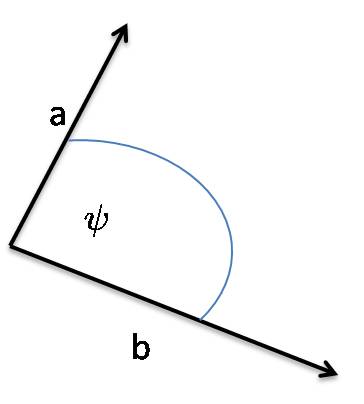
Figure C.1: Two vectors

Hence, anti-commutation takes a geometric meaning within the algebra: two vectors anti-commute if and only if they are orthogonal!

Similarly, we can write

$$a\wedge b=\frac{1}{2}\left[a,b\right]=\frac{1}{2}(ab-ba).$$

Geometrically, this means that two vectors are parallel if and only if they commute.

To gain some intuition, let’s look at the simple example of $\mathbb{R}^{2}$: Here, we have $a=a_{1}\Gamma_{1}+a_{2}\Gamma_{2}$ and $b=b_{1}\Gamma_{1}+b_{2}\Gamma_{2}$. The Clifford product of $a$ and $b$ is now given as

$$ab=\sum_{jk}a_{j}b_{k}\Gamma_{j}\Gamma_{k}=(a_{1}b_{1}+a_{2}b_{2})\mathbb{I}+(a_{1}b_{2}-b_{1}a_{2})\Gamma_{1}\Gamma_{2}.$$

The element $a\wedge b=(a_{1}b_{2}-b_{1}a_{2})\Gamma_{1}\Gamma_{2}$ represents the oriented plane segment of the parallelogram determined by $a$ and $b$ in Figure C.3 below. The area of this parallelogram is exactly $\left|a\wedge b\right|=|a_{1}b_{2}-b_{1}a_{2}|$. Note that we have $a\wedge b=-b\wedge a$, as shown in Figure C.3. Thus $a\wedge b$ not only gives us the area but also encodes a direction.

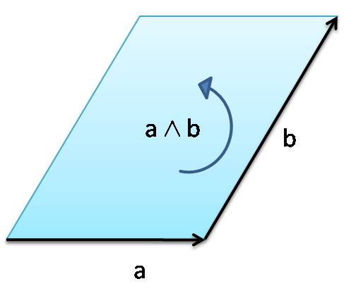
Figure C.2: $a\wedge b$

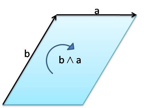
Figure C.3: $b\wedge a$

In higher dimensions, the elements generated by $a\wedge b\wedge c$ etc similarly correspond to oriented plane or volume segments. Note that we have $\Gamma_{i}\wedge\Gamma_{j}=\Gamma_{i}\Gamma_{j}$ for all basis vectors $\Gamma_{i}$ and $\Gamma_{j}$. We will refer to products of $k$ elements of the form $\Gamma_{i_{1}}\ldots\Gamma_{i_{k}}$ as $k$-vectors.

C.2.2 Reflections

The power of the Clifford algebra mainly lies in the fact that we can express geometrical operations involving any $k$-vector in an extremely easy fashion using the Clifford product. Here, we will only be concerned with performing operations on $1$-vectors.

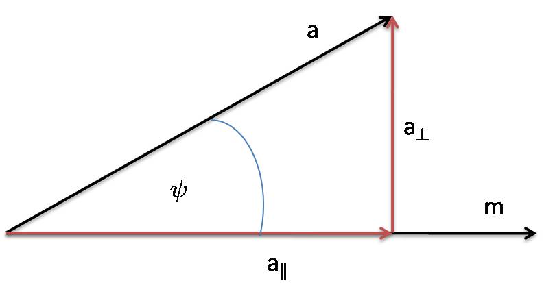
Figure C.4: Projections onto a vector

Consider the projection of a vector $a$ onto a vector $m$ as depicted in Figure C.4. Let $a_{\parallel}$ be the part of $a$ that is parallel to $m$, and $a_{\perp}$ the part of $a$ that lies perpendicular to $m$. Clearly, we may write $a=a_{\parallel}+a_{\perp}$. Using the definition of the Clifford product, we may write

$$a_{\parallel}=|a|\cos\psi\frac{m}{|m|}=(a\cdot m)m^{\dagger},$$

where we define $m^{\dagger}=m/|m|^{2}$ to be the inverse of $m$. Indeed, we have $mm^{\dagger}=\mathbb{I}$. If $m$ is a unit vector, then in terms of the matrix representation given above $m^{\dagger}$ is the adjoint of the matrix $m$. For the product of two vectors we define $(nm)^{\dagger}=m^{\dagger}n^{\dagger}$. We can also write

$$a_{\perp}=a-a_{\parallel}=a-(a\cdot m)m^{\dagger}=(am-(a\cdot m))m^{\dagger}=(a\wedge m)m^{\dagger}.$$

We can now easily determine the reflection of $a$ around the vector $m$, as depicted in Figure C.5:

$$t=a_{\parallel}-a_{\perp}=(a\cdot m-a\wedge m)m^{\dagger}=(m\cdot a+m\wedge a)m^{\dagger}=mam^{\dagger}.$$

Consider $n=1$. Then the $2$-dimensional real vector space is given by basis vectors $\Gamma_{1}=X$ and $\Gamma_{2}=Z$. Indeed, this is the familiar $XZ$-plane of the Bloch sphere depicted in Figure 2.1. Consider the Hadamard transform $H=(X+Z)/\sqrt{2}$. Figure C.7 demonstrates that $H$ plays exactly this role: it reflects $X$ around the vector $H$ to obtain $HXH=Z$. Given $t$, we can also easily derive the vector obtained by reflecting $a$ around the plane perpendicular to $m$ (in 0), as shown in Figure C.6.

$$-t=-mam^{\dagger}.$$

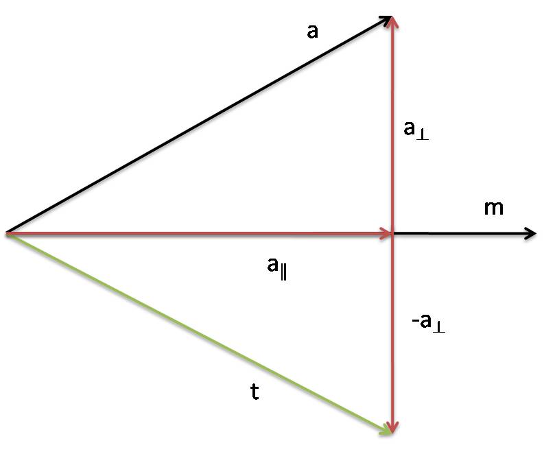
Figure C.5: Reflection of $a$ around $m$

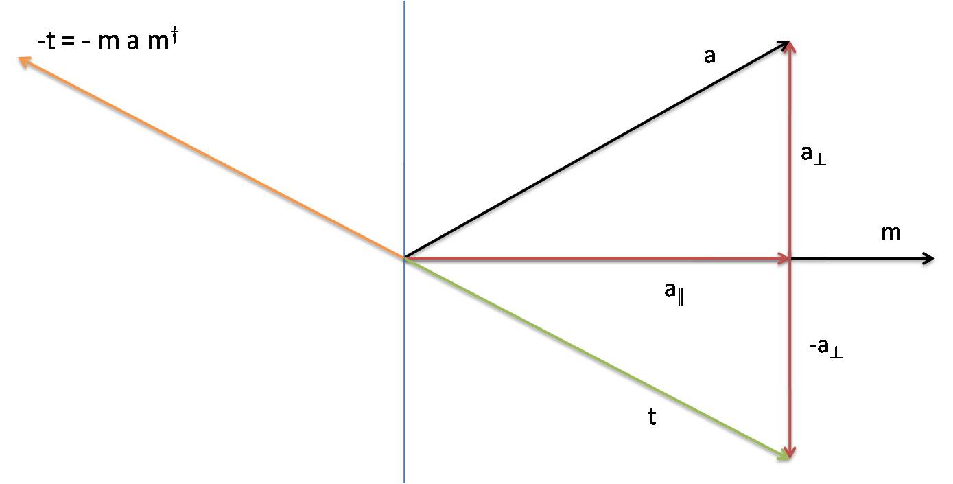
Figure C.6: Reflection of $a$ plane perpendicular to $m$

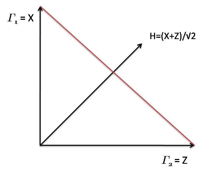
Figure C.7: Hadamard transform as reflection

C.2.3 Rotations

From reflections we may now obtain rotations as successive reflections. Suppose we are given vectors $m$ and $n$ as shown in Figure C.8. To rotate the vector $a$ by an angle that is twice the angle between $m$ and $n$, we now first reflect $a$ around $b$ to obtain $b=mam^{\dagger}$. We then reflect $b$ around $n$ to obtain

$$c=nbn^{\dagger}=nmam^{\dagger}n^{\dagger}=RaR^{\dagger},$$

where we let $R=nm$. As desired, $R$ rotates $a$ by an angle of $2(\psi+\phi)$.

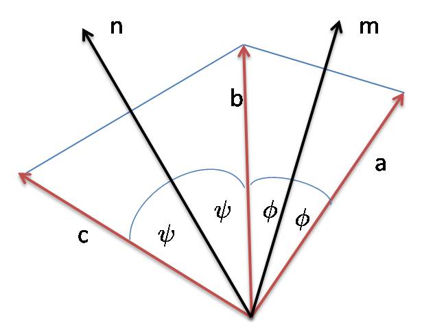
Figure C.8: Rotating in the plane $m\wedge n$.

We can easily convince ourselves that $R$ does not affect any vector $d$ that is orthogonal to both $n$ and $m$.

$$RdR^{\dagger}=nmdm^{\dagger}n^{\dagger}=dnmm^{\dagger}n^{\dagger}=d,$$

where we have used the fact that two vectors anti-commute if and only if they are orthogonal. Note also that $RR^{\dagger}=\mathbb{I}$. It can be shown that if $V$ is a $k$-vector, then $RVR^{\dagger}$ is also a $k$-vector for any rotation $R$ [DL03]. Indeed, this is easy to see, for the $k$-vector formed by orthogonal basis vectors:

$$R(\Gamma_{i_{1}}\wedge\ldots\wedge\Gamma_{i_{k}})R^{\dagger} = R(\Gamma_{i_{1}}\ldots\Gamma_{i_{k}})R^{\dagger}=R\Gamma_{i_{1}}R^{\dagger}\ldots R\Gamma_{i_{k}}R^{\dagger}$$

$$= R\Gamma_{i_{1}}R^{\dagger}\wedge\ldots\wedge R\Gamma_{i_{k}}R^{\dagger},$$

where we have used the fact that rotations preserve the angles between vectors. We will need this fact in our proof in Chapter 4.

Clifford algebra offers a very convenient way to express rotations around arbitrary angles in the plane $m\wedge n$ [Lou01]. In Chapter 4, however, we will only need to understand how we can find the rotation $R$ that takes us from a given vector $g=\sum_{j}g_{j}\Gamma_{j}$ with length $|g|$ to the vector $|g|\Gamma_{1}$. Indeed, our strategy works for finding the rotation of any vector $g$ to a target vector $t$ of the same length. Consider Figure C.9.

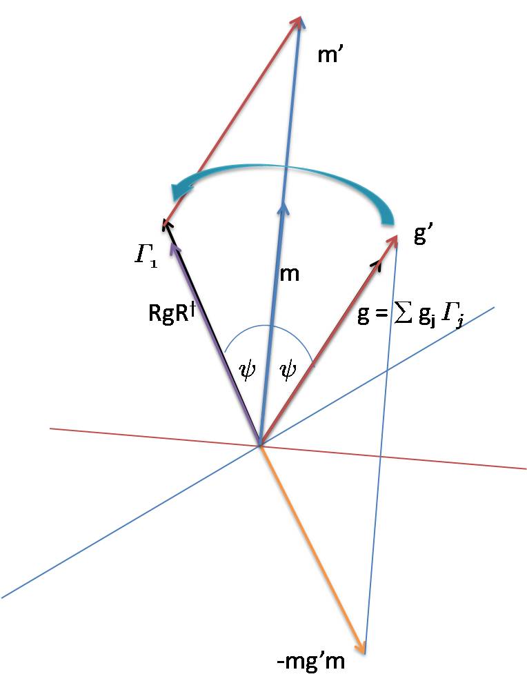
Figure C.9: Rotating $g$ to $|g|\Gamma_{1}$.

For convenience, we first normalize $g$ to obtain the vector

$$g^{\prime}=\frac{g}{|g|}.$$

We then compute the vector $m^{\prime}$ lying exactly half-way between $g^{\prime}$ and our target vector $\Gamma_{1}$ and normalize it to obtain

$$m=\frac{g^{\prime}+\Gamma_{1}}{|g^{\prime}+\Gamma_{1}|}=\frac{g^{\prime}+\Gamma_{1}}{\sqrt{2(1+g_{1}/|g|)}}.$$

We now first reflect $g^{\prime}$ around the plane perpendicular to the vector $m$ to obtain $-mg^{\prime}m$, followed by a reflection around the plane perpendicular to the target vector $\Gamma_{1}$:

$$-\Gamma_{1}(-mg^{\prime}m)\Gamma_{1}=\Gamma_{1}mg^{\prime}m\Gamma_{1}=Rg^{\prime}R^{\dagger},$$

with $R=\Gamma_{1}m$, where we have used the fact that both $\Gamma_{1}$ and $m$ have unit length and hence $m=m^{\dagger}$ and $\Gamma_{1}=\Gamma_{1}^{\dagger}$. Evidently,

$$Rg^{\prime}=\Gamma_{1}mg^{\prime} = \frac{1}{|g^{\prime}+\Gamma_{1}|}\Gamma_{1}(g^{\prime}+\Gamma_{1})g^{\prime}$$

$$= \frac{1}{|g^{\prime}+\Gamma_{1}|}\Gamma_{1}(g^{\prime 2}+\Gamma_{1}g^{\prime})=\frac{1}{|g^{\prime}+\Gamma_{1}|}(\Gamma_{1}+g^{\prime})=m,$$

and hence

$$Rg^{\prime}R^{\dagger}=mm\Gamma_{1}=\Gamma_{1}.$$

We then also have that

$$RgR^{\dagger}=|g|Rg^{\prime}R^{\dagger}=|g|\Gamma_{1}$$

as desired. We will employ a similar rotation in Chapter 4.

C.3 Application

Here, the primary benefit which we gain by considering a Clifford algebra, is that we can parametrize matrices in terms of its generators, and products thereof. Suppose we are given some matrix

$$\rho=\frac{1}{d}\left(\mathbb{I}+\sum_{j}b_{j}B_{j}\right),$$

where $\mathbb{I}\cup\{B_{j}\}$ form a basis for the $d\times d$ complex matrices, such that for all $j\neq j^{\prime}$ we have $\mbox{\rm Tr}(B_{j}B_{j^{\prime}})=0$, $\mbox{\rm Tr}(B_{j})=0$, $B_{j}^{2}=\mathbb{I}$, and $b_{j}\in\mathbb{R}$. We saw in Chapter 4 how to construct such a basis for $d=2^{n}$ based on mutually unbiased bases. In fact, this gives us the well-known Pauli basis, given by the $2^{2n}$ elements of the form $B_{j}=B_{j}^{1}\otimes\ldots\otimes B_{j}^{n}$ with $B_{j}^{i}\in\{\mathbb{I},\sigma_{x},\sigma_{y},\sigma_{z}\}$. When solving optimization problems within quantum information, we are often faced with the following problem: When is $\rho$ a quantum state? That is, what are the necessary and sufficient conditions for the coefficients $b_{j}$ such that $\rho\geq 0$?

For $d=2$, this is an easy problem: We can write $\rho=(\mathbb{I}+\sum_{j\in\{x,y,z\}}r_{j}\sigma_{j})/2$ where $\vec{r}=(r_{x},r_{y},r_{z})$ is the Bloch vector we encountered in Chapter 2. We have that $\rho\geq 0$ if and only if $-\mathbb{I}\leq\sum_{j}r_{j}\sigma_{j}\leq\mathbb{I}$, i.e.

$$\left(\sum_{j}r_{j}\sigma_{j}\right)^{2}=\frac{1}{2}\sum_{j,j^{\prime}}r_{j}r_{j^{\prime}}\{\sigma_{j},\sigma_{j^{\prime}}\}=\left(\sum_{j}r_{j}^{2}\right)\mathbb{I}\leq\mathbb{I}.$$

Thus, we have $\rho\geq 0$ if and only if $\sum_{j}r_{j}^{2}\leq 1$. Geometrically, this means that any point on or inside the Bloch sphere corresponds to a valid quantum state as illustrated in Figure 2.1. Sadly, when we consider $d>2$, our task becomes considerably more difficult. Clearly, since $\mbox{\rm Tr}(\rho^{2})\leq 1$ for any quantum state, we can always say that

$$\mbox{\rm Tr}(\rho^{2}) = \frac{1}{d^{2}}\left(\mbox{\rm Tr}(\mathbb{I})+2\sum_{j}b_{j}\mbox{\rm Tr}(B_{j})+\sum_{jj^{\prime}}b_{j}b_{j^{\prime}}\mbox{\rm Tr}(B_{j}B_{j^{\prime}})\right)$$

$$= \frac{1}{d^{2}}\left(d+\sum_{j}b_{j}^{2}\mbox{\rm Tr}(\mathbb{I})\right)$$

$$= \frac{1}{d}\left(1+\sum_{j}b_{j}^{2}\right)\leq 1,$$

giving us $\sum_{j}b_{j}^{2}\leq d-1$. Unfortunately, this condition is too weak for almost all practical applications. There exist many matrices which obey this condition, but nevertheless do not correspond to valid quantum states. Luckily, we can say something much stronger using the Clifford algebra.

Let’s consider the operators $\Gamma_{1},\ldots,\Gamma_{2n}$ themselves. Evidently, each operator $\Gamma_{i}$ has exactly two eigenvalues $\pm 1$: Let $|\eta\rangle$ be an eigenvector of $\Gamma_{i}$ with eigenvalue $\lambda$. From $\Gamma_{i}^{2}=\mathbb{I}$ we have that $\lambda^{2}=1$. Furthermore, we have $\Gamma_{i}(\Gamma_{j}|\eta\rangle)=-\lambda\Gamma_{j}|\eta\rangle$. Thus, if $\lambda$ is an eigenvalue of $\Gamma_{i}$ then so is $-\lambda$. We can therefore express each $\Gamma_{i}$ as

$$\Gamma_{i}=\Gamma_{i}^{0}-\Gamma_{i}^{1},$$

where $\Gamma_{i}^{0}$ and $\Gamma_{i}^{1}$ are projectors onto the positive and negative eigenspace of $\Gamma_{i}$ respectively. Furthermore, note that we have for all $i,j$ with $i\neq j$

$$\mbox{\rm Tr}(\Gamma_{i}\Gamma_{j})=\frac{1}{2}\mbox{\rm Tr}(\Gamma_{i}\Gamma_{j}+\Gamma_{j}\Gamma_{i})=0,$$

that is all such operators are orthogonal with respect to the Hilbert-Schmidt inner product. We now use the fact that the collection of operators

$$\begin{split}\mathbb{I}&\\ \Gamma_{j}&\phantom{===}(1\leq j\leq 2n)\\ \Gamma_{jk}&:=i\Gamma_{j}\Gamma_{k}\ (1\leq j<k\leq 2n)\\ \Gamma_{jk\ell}&:=\Gamma_{j}\Gamma_{k}\Gamma_{\ell}\ (1\leq j<k<\ell\leq 2n)\\ \vdots&\\ \Gamma_{12\ldots(2n)}&:=i\Gamma_{1}\Gamma_{2}\cdots\Gamma_{2n}=:\Gamma_{0}\end{split}$$

forms an orthogonal basis for the $d\times d$ matrices with $d=2^{n}$ [Die06]. By counting, the above operators form a complete operator basis with respect to the Hilbert-Schmidt inner product. In fact, by working out the individual basis elements with respect to the representation above, we see that this basis is in fact equal to the Pauli basis. Notice that the products with an odd number of factors are Hermitian, while the ones with an even number of factors are skew-Hermitian, so in the definition of the above operators we introduce a factor of $i$ to all with an even number of indices to make the whole set a basis for the Hermitian operators. Hence we can write every state $\rho\in\mathcal{H}$ as

$$\rho=\frac{1}{d}\left(\mathbb{I}+\sum_{j}g_{j}\Gamma_{j}+\sum_{j<k}g_{jk}\Gamma_{jk}+\ldots+g_{0}\Gamma_{0}\right),$$

with real coefficients $g_{j},g_{jk},\ldots$.

It is clear from the above that if we transform the generating set of $\Gamma_{j}$ linearly,

$$\Gamma_{k}^{\prime}=\sum_{j}T_{jk}\Gamma_{j},$$

then the set $\{\Gamma_{1}^{\prime},\ldots,\Gamma_{2n}^{\prime}\}$ satisfies the anti-commutation relations if and only if $(T_{jk})_{jk}$ is an orthogonal matrix: these are exactly the operations which preserve the inner product. In that case there exists a matching unitary $U(T)\in\mathbb{B}(\mathcal{H})$ which transforms the operator basis as

$$\Gamma_{j}^{\prime}=U(T)\Gamma_{j}U(T)^{\dagger}.$$

As an importance consequence, it can be shown [Die06] that any operation $U(T)$ transforms the state $\rho$ as

$$U(T)\rho U(T)^{\dagger}=\frac{1}{d}\left(\mathbb{I}+T(g)+\sum_{j<k}g^{\prime}_{jk}\Gamma_{jk}+\ldots+g^{\prime}_{0}\Gamma_{0}\right),$$

where we write $T(g)$ to indicate the transformation of the vector $g=\sum_{j}g_{j}\Gamma_{j}$ by $T$. For example, for the rotation $R$ constructed earlier, we may immediately write

$$R\rho R^{\dagger} = \frac{1}{d}\left(\mathbb{I}+RgR^{\dagger}+\sum_{j<k}g_{jk}R\Gamma_{jk}R^{\dagger}+\ldots+g_{0}R\Gamma_{0}R^{\dagger}\right),$$

$$= \frac{1}{d}\left(\mathbb{I}+|g|\Gamma_{1}+\sum_{j<k}g^{\prime}_{jk}\Gamma_{jk}+\ldots+g^{\prime}_{0}\Gamma_{0}\right),$$

Thus, we can think of the 1-vector components of $\rho$ as vectors in a generalized Bloch sphere. In Chapter 4, we will extend this approach to include the $\Gamma_{0}$ as an additional “vector”. There, we use these facts to prove a useful statement which leads to our uncertainty relations:

Lemma C.3.1 (Lemma 4.3.3).

For any state $\rho$, we have $\sum_{j}g_{j}^{2}\leq 1$.

With respect to our discussion above, this is indeed a generalization of what we observed for the Bloch sphere in $d=2$. Note that we obtain a whole range of such statements as we can find different sets of $2n$ anti-commuting matrices within the entire set of $2^{2n}$ basis elements above.

C.4 Conclusion

Luckily, we made some progress to give a characterization of quantum states in terms of their basis coefficients that was sufficient to prove our uncertainty relation from Chapter 4. Parametrizing states using Clifford algebra elements provides us with additional structure to characterize quantum states that is not at all obvious when looking at them from a linear algebra point of view alone. We hope that parametrizing states in this fashion could enable us to make even stronger statements in the future. It is also interesting to think about standard quantum gates as geometrical operations within the Clifford algebra. Indeed, this is possible to a large extent, but lies outside the scope of this text.

Clearly, the subspace spanned by the elements $\Gamma_{1},\ldots,\Gamma_{2n}$ plays a special role. Note that when considering the state minimizing our uncertainty relation, only its 1-vector coefficients played any role. The other coefficients do not contribute at all to the minimization problem. It is interesting to observe that we have in fact already seen a similar effect in Chapter 6. Recall that we used Tsirelson’s construction to turn vectors $a,b\in\mathbb{R}^{2n}$ back into observables by letting $A=\sum_{j}a_{j}\Gamma_{j}$ and $B=\sum_{j}b_{j}\Gamma_{j}$. The optimal strategy of Alice and Bob could then be implemented using the maximally entangled state of local dimension $d=2^{n}$

$$|\Psi\rangle\langle\Psi|=\frac{1}{d}\left(\mathbb{I}+\sum_{j}g_{j}\Gamma_{j}\otimes\Gamma_{j}+\sum_{j}r_{j}R_{j}\otimes R_{j}\right),$$

where $g_{j}=\pm 1$ and we used the $R_{j}$ simply as a remainder term. Clearly, the coefficients $r_{j}$ do not contribute to the term $\langle\Psi|A\otimes B|\Psi\rangle$ at all, and only the coefficients $g_{j}$ matter. However, in dimension $d=2^{n}$ we have only $2n$ such terms. Curiously, the remaining terms are only needed to ensure that $\rho\geq 0$. Numerical feasibility analysis using semidefinite programming for $d=4$ and $d=8$ reveals that we do indeed need to take the maximally entangled state, and cannot omit any of the remaining terms.

Index

• $*$-algebra §B.2
• $\oplus\mbox{MIP}[2]$ Definition 9.2.1
• $\oplus\mbox{MIP}^{*}$ §9.1.2
• $\oplus{\mbox{MIP}}^{*}[2]$ Definition 9.2.2, Theorem 9.3.1
• $\oplus\mbox{MIP}_{\mbox{\tiny{NL}}}$ §9.1.2
• 1-2 oblivious transfer Definition 1.3.3
• 1-2 OT Definition 1.3.3
  • practical §11.4
• accessible information §2.3.2
• adversary §1.2.1
• adversary model §11.1
• algebra
  • $*$-algebra §B.2
  • Banach §B.2
  • $C^{*}$-algebra §B.2
  • center §B.4
  • commutant §B.4
  • GNS construction Theorem B.3.1
  • ideal §B.2
  • invertible §B.2
  • observable §B.3.1
  • positive linear functional §B.3.1
  • pure state §B.3.1
  • semisimple §B.2
  • simple §B.2
  • spectrum §B.2
  • state §B.3.1
  • state space §B.3.1
  • unital §B.2
• anonymous transmissions §1.3.4
• anti-commuting observables §C.1, §4.3
• Banach algebra §B.2
• basis §A.1
  • Breidbart §11.2.1
  • computational §2.1.1
  • Hadamard §2.1.1
  • measurement in §2.1.3
  • MUB §2.4, Lemma 4.2.8
  • mutually unbiased §2.4
• basis vectors §A.1
• BB84 §1.1, §11.1
• BC Definition 1.3.1
• Bell inequalities §6.2.2
• Bell inequality §6.1.1
  • CHSH §6.1.1
• binary entropy §2.3.1
• bipartite state §2.1.2
  • mutual information §2.3.1
• bipartite structure §B.4.2
• bit commitment §1.3.1, Definition 1.3.1
  • impossibility §10.2.3
  • limitations Chapter 10
• bit string commitment §1.3.1
  • impossibility §10.3
  • possibility §10.4
• Bloch sphere §2.2
• Bloch vector §2.2
• bounded operator §A.1
• bounded storage
  • classical §1.2.2
  • composability §1.4
  • due to noise Chapter 11
  • quantum §1.3.1, §11.1, §3.1
• Boykin, P. O. §1.3.4
• Breidbart basis §11.2.1
• $C^{*}$-Algebra Appendix B, §B.2
• center §B.4
• cheat-sensitive item 2, §1.3.1, §2.1.3
• CHSH inequality §6.1.1, §7.2
  • generalized §7.3
• classical ensemble §2.1.1
• classical information §2.1.3
• classical mutual information §2.3.1
• Clifford algebra Appendix C, §C.1, §4.3
  • generators §C.1
  • geometrical properties §C.2
  • product §C.2
  • uncertainty relation §4.3
• Clifford product §C.2
• coin tossing
  • strong Definition 1.3.5
  • weak Definition 1.3.6
• collision entropy §2.3.1
• commitment
  • bit Definition 1.3.1
  • quantum bit string Definition 10.2.1
• commutant §B.4
• compatible §B.4
• complementary §B.4
• complete §6.1
• complex Hadamard matrix §2.4.1
• composability §1.4
  • bounded storage §1.4
• computational basis §2.1.1
• computational security §1.2.2
• conditional entropy §2.3.1
• cone §A.2
• conjugate transpose §A.1
• convex cone §A.2
• CP map §2.1.3
• CPTP map §2.1.3
• cq-state §11.2.1
• cryptography Chapter 1
• data hiding §1.3.3
• density matrix §2.1.1
• density operator §2.1.1
• depolarizing channel §11.5
• depolarizing noise §11.5
• dishonest §1.2.1
• distance
  • from uniform §11.2.1
  • trace Definition 2.2.1
  • variational §2.2
• distinguishability §2.2
• disturb §2.1.3
• dual §A.3
• dual function §A.3
• duality §A.3
  • strong §A.3
  • weak §A.3
• E91 §1.1
• eigendecomposition §A.1
• eigenvalue §A.1
• eigenvector §A.1
• encoding §2.1.1
• ensemble §2.1.1
  • classical §2.1.1
• entanglement item 5, Chapter 6
• entropy
  • binary §2.3.1
  • collision §2.3.1
  • conditional §2.3.1
  • joint §2.3.1
  • min-entropy §2.3.1
  • Rényi §2.3.1
  • Shannon §2.3.1
  • von Neumann §2.3.2
• EPR §6.1
  • pair 6.1
  • Paradox §6.1
  • state 6.1
• feasible §A.3
• fidelity Definition 2.2.3
• games
  • non-local §6.2.3
  • optimal strategies Chapter 7
  • superposition §9.4
  • XOR §6.2.3
  • XOR, winning probability 9.2
• generalized Pauli matrices §2.4.2
• GNS construction Theorem B.3.1
• $H_{2}(\cdot\mid\cdot)$ §10.2.3
• Hadamard basis §2.1.1
• Hadamard transform §2.1.3
• Hermitian §A.1
• hidden variables §6.1
• Hilbert space §A.1
  • bounded operators §B.2
• Holevo quantity §2.3.2
• honest §1.2.1
• honest-but-curious §1.2.1, §2.1.3
• ideal §B.2
• impossibility
  • bit commitment §10.2.3
  • bit string commitment Theorem 10.3.1
• information
  • accessible §2.3.2
  • mutual §2.3.1
• information theoretic security §1.2.2
• inner product §A.1
• instrument §2.1.3
• interactive proof system Chapter 9
• invertible §B.2
• IP §9.1.1
• joint entropy §2.3.1
• Jordan Wigner transformation §C.1
• K-transform §2.1.3
• $k$-vector §C.2.1
• Kraus operator §2.1.3
• Lagrangian §A.3
• Latin square §2.4.1
  • mutually orthogonal §2.4
• left ideal §B.2
• LOCKCOM §10.4
• locking item 4, Chapter 5
  • application §10.4
  • mutually unbiased bases §5.2
  • protocol §5.1.1
  • uncertainty relations §5.1.2
• measurement §2.1.3
  • delay item 6
  • in a basis §2.1.3
  • observable §2.1.3
  • operators §2.1.3
  • post-measurement state §2.1.3
  • POVM §2.1.3
  • projective §2.1.3
• min-entropy §2.3.1
• MIP §9.1.1
• MIP[2] §9.1.1
• mixed state §2.1.1
• mixture §2.1.1
• MOLS §2.4
• MUB §2.4
  • from Latin squares §2.4.1
  • from Pauli matrices §2.4.2
• mutual information §2.3.1
  • classical §2.3.1
• mutually unbiased basis §2.4
  • from Latin squares §2.4.1
  • from Pauli matrices §2.4.2
• no-cloning item 1, §2.1.1
• noise
  • depolarizing §11.5
• noisy channel §1.2.2
• noisy quantum storage model §11.1
• noisy storage Chapter 11
• non-local games §6.2.3
• non-uniformity §11.2.1
• oblivious transfer §11.1
  • 1-2 Definition 1.3.3
  • practical §11.4
  • Rabin Definition 1.3.4
• observable §B.3.1, §2.1.3
  • algebra §B.3.1
  • anti-commuting §4.3
  • compatible §B.4
  • complementary §B.4
• operator norm §A.1
• orthogonal projector §A.2
• OT §11.1
  • 1-2 Definition 1.3.3
  • Rabin Definition 1.3.4
• outer product §C.2.1
• Pauli matrices §2.1.3
  • generalized §2.4.2
  • strings of §2.4.2
• perfect secrecy §1.2.2
• physical reality §6.1
• PI-STAR Definition 3.2.2, §6.4, Lemma 6.4.1
  • algebraic framework §3.5.1
  • AND §3.4.2
  • gap §6.4
  • lower bound §3.4.1
  • no quantum memory §3.4
  • perfect prediction §3.5.1
  • quantum memory §3.5
  • three bases §3.5.3
  • to succeed at §3.2.2
  • two bases §3.5.2
  • XOR §3.4.2
• player §1.2.1
• positive definite §A.2
• positive linear functional §B.3.1
• positive semidefinite §A.2
• post-measurement information Chapter 3, Definition 3.2.2
  • algebraic framework §3.5.1
  • AND §3.4.2
  • gap §6.4
  • lower bound §3.4.1
  • no quantum memory §3.4
  • perfect prediction §3.5.1
  • quantum memory §3.5
  • three bases §3.5.3
  • two bases §3.5.2
  • XOR §3.4.2
• post-measurement state §2.1.3
• POVM §2.1.3
• primal §A.3
• privacy amplification §10.2.3, Theorem 10.2.4
• private input §1.2.1
• private shared input §1.2.1
• private shared randomness §1.2.1
• projective measurement §2.1.3
• projector §A.2
  • orthogonal §A.2
• public information §1.2.1
• pure state §2.1.1
• purification §2.1.2
• QBSC Definition 10.2.1
  • impossibility Theorem 10.3.1
  • possibility §10.4
• QIP §9.1.1
• QIP(2) §9.1.2, Definition 9.2.3
• QKD §1.1, §1.3
• quantum bit string commitment Definition 10.2.1
• quantum channel §2.1.3
  • trace preserving §2.1.3
  • unital §2.1.3
• quantum key distribution §1.1, §1.3
• quantum seals §1.3.5
• quantum signatures §1.3.5
• quantum strategy Chapter 7
• qubit §2.1.1
• RAC §8.2.1
• random access code §8.2.1
  • unbalanced Definition 8.2.2
• randomized oblivious transfer Definition 11.2.1
• rank §A.1
• reduced state §2.1.2
• Rényi entropy §2.3.1
• right ideal §B.2
• ROT Definition 11.2.1
• SDP §A.3
  • dual §A.3
  • dual function §A.3
  • duality §A.3
  • example §2.2, Proof 3.4.11, Proof 3.4.5, Proof 3.4.5
  • feasible §A.3
  • Lagrangian §A.3
  • primal §A.3
  • Slater’s conditions §A.3
  • standard form §A.3
  • strong duality §A.3
  • weak duality §A.3
• secret
  • classical §1.3.3
  • quantum §1.3.3
• secret sharing §1.3.3
• secure function evaluation Definition 1.3.2
• secure multi-party computation §1.3.2
• semidefinite program (SDP) §A.3
• semidefinite programming Appendix A
• semisimple §B.2
  • decomposition Lemma B.4.1
• SFE Definition 1.3.2
• Shannon entropy §2.3.1
• simple §B.2
• SMP §1.3.2
• spectrum §B.2
• STAR Definition 3.2.1, §6.4, Lemma 6.4.1
  • AND §3.3.3
  • Boolean functions §3.3.2
  • to succeed at §3.2.2
  • XOR §3.3.4
• state
  • algebra §B.3.1
  • bipartite §2.1.2
  • discrimination §2.2
  • discrimination with post-measurement information Chapter 3
  • EPR pair 6.1
  • invariant §B.4.3
  • mixed §2.1.1
  • post-measurement §2.1.3
  • pure §B.3.1, §2.1.1
  • reduced §2.1.2
  • von Neumann entropy §2.3.2
  • Werner §6.2.1
• state discrimination Definition 3.2.1
  • AND §3.3.3
  • Boolean functions §3.3.2
  • with post-measurement information Definition 3.2.2
  • XOR §3.3.4
• state space §B.3.1
• string commitment Chapter 10
• string of Pauli matrices §2.4.2
• strong duality §A.3
• superoperator §2.1.3
• superposition game §9.4
• superselection rules §1.2.2, §1.3.1
• tensor product §A.1
• trace §A.1
• trace distance Definition 2.2.1
• trace norm Definition 2.2.1
• trace out §2.1.2
• traceless §1.3.4
• transpose §A.1
• trusted initializer §1.2.2
• Tsirelson
  • bound §6.1.2, §7.2
  • construction Theorem 6.3.6, §7.1
  • vectors Theorem 6.3.6
• two-party protocols §10.2.2
• two-sided ideal §B.2
• two-universal hash function §10.2.3
• uncertainty Chapter 4
• uncertainty relation item 3, Chapter 4
  • Clifford algebra §4.3
  • for all MUBs Theorem 4.2.14
  • for anti-commuting observables §4.3
  • for Latin square MUBs Lemma 4.2.6
  • for MUBs in square dimensions Theorem 4.2.4
  • for two bases Theorem 4.2.1
  • Heisenberg §4.1
  • Maassen and Uffink Theorem 4.2.1
  • meta §4.3.2
• unconditional security §1.2.2
• unforgeable subway tokens §1.1, §1.3.5
• unital
  • algebra §B.2
  • quantum channel §2.1.3
• unitary §A.1
• unitary evolution §2.1.3
• URAC Definition 8.2.2
• variational distance §2.2
• verifier §6.2.3
• von Neumann entropy §2.3.2
• weak duality §A.3
• Werner state §6.2.1

List of Figures

1. 1.1 Introduction
2. 1.3 Schematic run of a BC protocol when Alice and Bob are honest.
3. 1.4 Schematic run of a 1-2 OT protocol.
4. 2.1 Bloch vector $(r_{x},r_{y},r_{z})=(\cos\psi\sin\theta,\sin\psi\sin\theta,\cos\theta)$
5. 2.4.1 Latin squares
6. 3.1 Using post-measurement information.
7. 4.1 2n = 2-cube
8. 4.2 2n = 4-cube
9. 5.1 A locking protocol for 2 bases.
10. 5.2 Measurement for $|1,1\rangle$.
11. 6.1 Alice and Bob measure many copies of $|\Psi\rangle$
12. 6.2 Multiplayer non-local games.
13. 6.4 The use of post-measurement information
14. 7.1 Optimal vectors for $n=4$ obtained numerically using Matlab.
15. 8.1 Tradeoff for $p=0.6$.
16. 8.2 Tradeoff for 2 outcomes.
17. 9.1 A one-round XOR proof system.
18. 10.1 Moving from a set of string with $g(x)=y$ to a set of strings with $g(x)=(y\mod 5)+1$.
19. 11.1 Bob performs a partial measurement $\mathcal{P}_{i}$, followed by noise $\mathcal{N}$, and outputs a guess bit $x_{g}$ depending on his classical measurement outcome, the remaining quantum state, and the additional basis information.
20. 11.2 $h((1-ar)/2)/4+\log(\frac{1+r}{2})\log(4/3)/2$, where we only show the region below 0, i.e., where security can be attained.
21. C.1 Two vectors
22. C.2.1 Inner and outer product
23. C.4 Projections onto a vector
24. C.5 Reflection of $a$ around $m$
25. C.6 Reflection of $a$ plane perpendicular to $m$
26. C.7 Hadamard transform as reflection
27. C.8 Rotating in the plane $m\wedge n$.
28. C.9 Rotating $g$ to $|g|\Gamma_{1}$.

Symbol		Page
$\log$	binary logarithm
$\ln$	natural logarithm
$a^{*}$	complex conjugate of $a$
$|a|$	absolute value of $a$
$|\mathcal{S}|$	number of elements of the set $\mathcal{S}$
$\mathbb{N}$	set of natural numbers $1,2,3,\ldots$
$\mathbb{R}$	set of real numbers
$\mathbb{C}$	set of complex numbers
$[n]$	set of numbers $\{1,\ldots,n\}$
$x_{|\mathcal{S}}$	string $x$ restricted to the indices in $\mathcal{S}$
$\delta_{ij}$	$\delta_{ij}=1$ if $i=j$ and $\delta_{ij}=0$ otherwise
$\mathbb{I}$	identity matrix
$\mathbb{I}_{d}$	$d\times d$ identity matrix
$A^{[1]}$	matrix $A$ acting on subsystem 1
$A^{-1}$	inverse of the matrix $A$
$A^{T}$	transpose of the matrix $A$
$A^{*}$	conjugate of the matrix $A$
$A^{\dagger}$	conjugate transpose of the matrix $A$
$[a_{ij}]$	matrix whose entry in the $i$-th row and $j$-th column is $a_{ij}$
$\mbox{\rm Tr}(A)$	trace of $A=[a_{ij}]$ given by $\sum_{j}a_{jj}$
$\mbox{rank}(A)$	rank of the matrix $A$
$A>0$	$A$ is positive definite	A.2
$A\geq 0$	$A$ is positive semidefinite	A.2
$||A||_{1}$	trace norm of $A$, given by $\mbox{\rm Tr}\sqrt{A^{\dagger}A}$
$\vec{a}$	real vector $\vec{a}=(a_{1},\ldots,a_{d})$
$|\Psi\rangle$	complex vector $|\Psi\rangle=(\alpha_{1},\ldots,\alpha_{d})$
$|x_{b}\rangle$	string $x$ encoded in basis $b$
$\langle{\Psi}|{\Phi}\rangle$	inner product of $|\Psi\rangle$ and $|\Phi\rangle$
$x\cdot y$	standard inner product of real vectors $x$ and $y$
$|\Psi\rangle\langle\Phi|$	outer product of $|\Psi\rangle$ and $|\Phi\rangle$
$|\Psi\rangle\langle\Psi|$	projector onto the vector $|\Psi\rangle$
$|||\Psi\rangle||$	2-norm given by $\sqrt{\langle{\Psi}|{\Psi}\rangle}$
$\mathcal{H}$	a Hilbert space
$\mathbb{B}(\mathcal{H})$	set of all bounded operators on $\mathcal{H}$
$\mathcal{S}(\mathcal{H})$	set of states on $\mathcal{H}$
$[A,B]$	commutator $AB-BA$
$\{A,B\}$	anti-commutator $AB+BA$
$\mbox{Comm}(\mathscr{A})$	commutant of the algebra $\mathscr{A}$	B.4
$\mathcal{Z}_{\mathscr{A}}$	center of the algebra $\mathscr{A}$	B.4
$\langle A_{1},\ldots,A_{n}\rangle$	algebra generated by $A_{1},\ldots,A_{n}$	2
$\langle\mathcal{S}\rangle$	algebra generated by operators from the set $\mathcal{S}$	2
$D(\rho,\sigma)$	trace distance of $\rho$ and $\sigma$	2.2.1
$F(\rho,\sigma)$	fidelity of $\rho$ and $\sigma$	2.2.3
$d(X|\rho)$	distance from uniform of r.v. $X$ given state $\rho$	11.2.1
$h(p)$	binary entropy	2.3.1
$H(X,Y)$	joint entropy of $X$ and $Y$	2.3.1
$H(X|Y)$	conditional entropy of $X$ given $Y$	2.3.1
$\mathcal{I}(X,Y)$	mutual information of $X$ and $Y$	2.3.1
$\mathcal{I}_{c}(\rho_{AB})$	classical mutual information of $\rho_{AB}$	2.3.1
$\mathcal{I}_{acc}(\mathcal{E})$	accessible information of an ensemble $\mathcal{E}$	2.3.2
$S(\rho)$	von Neumann entropy of the state $\rho$	2.3.2
$\chi(\rho)$	Holevo quantity	2.3.2
$H_{\infty}(X)$	min-entropy	2.3.1
$H_{2}(X)$	collision entropy	2.3.1
$H_{2}(\rho_{AB}|\rho_{B})$	collision entropy of $\rho_{AB}$ given $\rho_{B}$	10.2.3

Quantum computing heeft een grote invloed op cryptografie gehad. Met de ontdekking van Shors quantum algorithme voor het factoriseren van grote getallen kunnen opeens bijna alle klassieke systemen gebroken worden zodra een quantum computer is gebouwd. Het is daarom belangrijk om andere manieren te verzinnen om veilige cryptografische protocollen te kunnen implementeren. Dit proefschrift draagt ertoe bij om zowel de fysieke beperkingen, als ook de mogelijkheden van cryptographie in een quantum omgeving beter te begrijpen. Wij bekijken eerst twee aspecten die een cruciale rol spelen voor de veiligheid van quantum protocollen: onzekerheidsrelaties en quantum entanglement. Hoe kunnen wij goede onzekerheidsrelaties voor een groot aantal meetinstellingen vinden? Wat is het effect van entanglement op klassieke protocollen? En, welke beperkingen legt entanglement quantum protocollen op? Ten slotte, kunnen wij deze beperkingen omzeilen onder realitische aanames?

Informatie in quantum toestanden

In dit deel houden wij ons bezig met het extraheren van informatie uit quantum toestanden. Een van de meest fundamentele doelen is het onderscheiden van quantum toestanden. Gegeven een set van mogelijke toestanden, wat is de toestand die wij op dit moment voor handen hebben? Wij bestuderen een variant van dit probleem dat van belang is voor de veiligheid van protocollen in het bounded quantum storage model. We ontvangen na de meting, of meer algemeen nadat een quantum memory bound toegepast wordt, nog extra informatie. Wij introduceren een algemeen algebraisch raamwerk, dat het mogelijk maakt om dit probleem voor elke set van toestanden op te lossen en geven twee voorbeelden.

Verder onderzoeken wij entropische onzekerheidsrelaties, die een andere manier vormen om Heisenberg’s onzekerheids principe te beschrijven. Dit is meestal een beter manier om “onzekerheid” te beschrijven aangezien de ondergrens niet afhangt van een bepaald toestand maar alleen van de metingen zelf. Entropische onzekerheidsrelaties hebben recentelijk meer invloed gekregen binnen het veld van quantum cryptografie in het bounded storage model, waar de veiligheid van protocollen uiteindelijk afhangt van zulke onzekerheidsrelaties. Dus nieuwe onzekerheidsrelaties kunnen tot nieuwe protocollen leiden.

Onzekerheidrelaties zijn bekend voor twee of $d+1$ wederzijds “unbiased measurements”. Wij bewijzgn eerst nauwe entropische onzekerheidsrelaties voor metingen met een groot aantal “mutually unbiased bases” (MUBs) in dimensionen $d=s^{2}$. Wij laten ook zien dat MUBs geen goede keuze zijn voor “locking” van klassieke informatie in quantum toestanden; ook als wij meer dan twee van zulke MUBs gebruiken neemt het locking effect niet toe.

Onze resultaten laten zien dat men heel voorzichtig dient te zijn om “maximaal incompatibele” metingen als wederzijds “unbiased” te veronderstellen. Maar welke eigenschappen moeten een meting hebben om heel ‘incompatibel’ te zijn? Gelukkig kunnen wij zulke eigenschappen vinden voor metingen met twee uitkomsten. Voor anti-commuterende metingen die generatoren van een Clifford algebra vormen, bewijzen wij optimale onzekerheidsrelaties voor de Shannon entropie, en bijna optimale relaties voor de collision entropie. Onze resultaten kunnen worden toegepast op quantum cryptographie.

Entanglement

In dit deel onderzoeken wij quantum entanglement. Allereerst, kijken wij naar Tsirelson inequalities. Wij laten zien hoe wij de optimale strategie voor spelletjes met twee uitkomsten met behulp van semidefinite programming kunnen bepalen. Als voorbeeld laten wij een upper bound voor de gegeneraliseerde CHSH ongelijkheid zien.

Verder laten wij zien hoe klassieke interactieve bewijssystemen met twee spelers (provers) kunnen veranderen als de spelers entanglement kunnen delen. Dit is een voorbeeld van hoe de veiligheid van klassieke systemen kan veranderen, ook al is het alleen mogelijk een beperkt soort quantum operaties uit te voeren: Het bewijssysteem wordt significant verzwakt ook al hebben de spelers geen toegang tot een quantum computer.

Applicaties voor de cryptografie

In deel IV onderzoeken wij de consequenties van onzekerheidsrelaties en entanglement in quantum systemen voor de cryptografie. Traditioneel houdt de cryptografie zich vooral bezig met het veilig versturen van berichten. Maar met de opkomst van het internet zijn nieuwe taken van belang geworden. Wij willen protocollen creeren voor het elektronisch stemmen, online veilingen, ondertekenen van contracten en vele andere applicaties, waarbij de deelnemers elkaar niet vertrouwen. De focus ligt daarbij op twee primitieven, met behulp waarvan wij al deze problemen kunnen oplossen: bit commitment en oblivious transfer. Klassieke protocollen voor deze primitieven zijn gebaseerd op computationele aanames die met behulp van een quantum computer gebroken kunnen worden. Helaas is het bekend dat zelfs in de quantum wereld deze primitieven niet helemaal zonder aannames geimplementeerd kunnen worden. Wat hopen wij dan wel te kunnen bereiken?

Als bit commitment onmogelijk is, kunnen wij misschien de taak een klein beetje aanpassen en dan nuttige protocollen vinden? Hier bekijken wij commitments van een hele string van bits tegelijk, waar de tegenstander niet is beperkt. Als bit commitment onmogelijk is, is perfecte string commitment ook niet mogelijk. Maar wij geven elke tegenstander de mogelijkheid om een beetje vals te spelen. Wij geven een raamwerk voor een familie van string commitment protocollen. Hoe wij informatie meten blijkt een cruciale rol te spelen; voor een heel sterke maat van informatie laten wij zien dat zelfs deze imperfecte string commitments niet mogelijk zijn. Maar voor een zwakkere manier om informatie te meten construeren wij toch niet-triviale protocollen die klassiek niet mogelijk zijn.

Ten slotte laten wij zien dat bit commitment en oblivious transfer wel mogelijk worden, indien wij de tegenstander realistische beperkingen opleggen. Wij introduceeren het noisy-storage model, dat nauw is gerelateerd aan het bounded-storage model. Wij laten zien dat het mogelijk is om oblivious transfer te implementeren, zolang de tegenstander qubits niet zonder fouten kan opslaan. Gegeven de status van de experimentele mogelijkheden vandaag de dag, lijkt dit een realistische aanname, maar is afhankelijk van de implementatie moeilijk te bepalen. Dezelfde problemen die het ook zo moeilijk maken om een quantum computer te bouwen komen ons hier ten goede!

Information in Quantum States

In this part, we start by investigating how to extract information from quantum states. One of the most basic tasks is the discrimination of quantum states. Given an ensemble of known quantum states, which one do we hold in our hands? We study a variant of this problem which is of central importance for the security of protocols in the bounded-quantum-storage model. Here, we are given additional information about the state after the measurement or, more generally, after a quantum memory bound is applied. We prove general bounds on the success probability which answer in the negative the question whether deterministic privacy amplification is possible in all known protocols in the bounded-quantum-storage model. To this end, we introduce a general algebraic framework which allows us to solve this problem for any set of states and provide two explicit examples.

We then turn to examine entropic uncertainty relations, which are an alternative way to state Heisenberg’s uncertainty principle. They are frequently a more useful characterization, because the “uncertainty” is lower bounded by a quantity that does not depend on the state to be measured. Recently, entropic uncertainty relations have gained importance in the context of quantum cryptography in the bounded-storage model, where proving the security of protocols ultimately reduces to bounding such relations. Proving new entropic uncertainty relations could thus give rise to new protocols. Such relations are known for two or $d+1$ mutually unbiased measurements. We prove tight entropic uncertainty relations for measurements in a large number of specific mutually unbiased bases (MUBs) in square dimensions. In a similar way, we show that such MUBs are unsuitable for locking classical correlations in quantum states: Using 2 or all of them does not increase the locking effect.

Our result shows that one needs to be careful about thinking of “maximally incompatible” measurements as being necessarily mutually unbiased. But what properties do measurements need to have in order to give strong uncertainty relations? We find very strong uncertainty relations from the generators of a Clifford algebra. In particular, we prove that for $k$ such anti-commuting observables $X_{1},\ldots,X_{k}$ we obtain optimal uncertainty relations for the Shannon entropy and nearly optimal relations for the collision entropy. Our results have immediate applications to quantum cryptography in the bounded-storage model.

Entanglement

In this part, we investigate the intriguing notion of quantum entanglement. We demonstrate how to find the optimal quantum strategies for correlation inequalities where each measurement has exactly two outcomes using semidefinite programming. As an example, we prove a tight upper bound for a well-known generalized CHSH inequality.

Furthermore, we consider how a classical two-prover interactive proof system changes if the provers are allowed to share entanglement. In this setting, a polynomial time bounded verifier is allowed to ask questions to two unbounded provers, who are trying to convince the verifier of the validity of a specific statement, even if the statement is false. The provers may thereby agree on any strategy ahead of time, but can no longer communicate once the protocol starts. Surprisingly, it turns out that, when the provers are allowed to share entanglement, it is possible to simulate two such classical provers using a single quantum prover. This indicates that entanglement among provers truly weakens the proof system, and provides an example of how classical systems can be affected, even if we only allow a very limited set of quantum operations.

Applications to Cryptography

In this part, we consider the consequences of uncertainty relations and entanglement in quantum systems to cryptography. Traditional cryptography is concerned with the secure and reliable transmission of messages. With the advent of widespread electronic communication and the internet, however, new cryptographic tasks have become increasingly important. We would like to construct secure protocols for electronic voting, online auctions, contract signing and many other applications where the protocol participants themselves do not trust each other. main focus is on two primitives, which form an important building block for constructing multi-party protocols: bit commitment and oblivious transfer. Classical protocols for such problems are usually based on computational assumptions which do not stand up to a quantum computer. Unfortunately, it has been shown that even quantum computers do not help in this case and that perfect quantum bit commitment and oblivious transfer are impossible. In the face of such negative statements, what can we still hope to achieve?

Given that perfect bit commitment is impossible, perhaps we can alter the task slightly and obtain useful protocols? Here, we considered commitments to an entire string of bits at once, when the attacker has unbounded resources at his disposal. Evidently, if perfect bit commitment is impossible, perfect string commitment is also impossible as well. However, we showed that we can obtain non-trivial quantum protocols, where the participants have a small ability to cheat. To this end, we introduced a framework for the classification of string commitment protocols. In particular, we proved that the measure of information is crucial to the security: For a very strong notion of security, we showed that even slightly imperfect quantum string commitments are also impossible. Nevertheless, we showed that for a weaker measure of information we can indeed obtain nontrivial protocols, which are impossible in a classical world.

Luckily, it turns out that we can implement oblivious transfer if we are willing to assume that storing qubits is noisy. We introduce the model of noisy quantum storage, which is similar to the model of bounded quantum storage. Here, however, we consider an explicit noise model inspired by present day technology. If the honest parties can perform perfect quantum operations, then we show that the protocol is secure for any amount of noise. In case the honest participants are only able to perform noisy operations themselves, we analyze a practical protocol that can be implemented using present-day hardware. We show how to derive explicit tradeoffs between the amount of storage noise, the amount of noise in the operations performed by the honest participants and the security of the protocol. Here, the very problem that makes it so hard to implement a quantum computer can actually be turned to our advantage.

Titles in the ILLC Dissertation Series:

• Maria Aloni
  Quantification under Conceptual Covers

• Alexander van den Bosch
  Rationality in Discovery - a study of Logic, Cognition, Computation and Neuropharmacology

• Erik de Haas
  Logics For OO Information Systems: a Semantic Study of Object Orientation from a Categorial Substructural Perspective

• Rosalie Iemhoff
  Provability Logic and Admissible Rules

• Eva Hoogland
  Definability and Interpolation: Model-theoretic investigations

• Ronald de Wolf
  Quantum Computing and Communication Complexity

• Katsumi Sasaki
  Logics and Provability

• Allard Tamminga
  Belief Dynamics. (Epistemo)logical Investigations

• Gwen Kerdiles
  Saying It with Pictures: a Logical Landscape of Conceptual Graphs

• Marc Pauly
  Logic for Social Software

• Nikos Massios
  Decision-Theoretic Robotic Surveillance

• Marco Aiello
  Spatial Reasoning: Theory and Practice

• Yuri Engelhardt
  The Language of Graphics

• Willem Klaas van Dam
  On Quantum Computation Theory

• Rosella Gennari
  Mapping Inferences: Constraint Propagation and Diamond Satisfaction

• Ivar Vermeulen
  A Logical Approach to Competition in Industries

• Barteld Kooi
  Knowledge, chance, and change

• Elisabeth Catherine Brouwer
  Imagining Metaphors: Cognitive Representation in Interpretation and Understanding

• Juan Heguiabehere
  Building Logic Toolboxes

• Christof Monz
  From Document Retrieval to Question Answering

• Hein Philipp Röhrig
  Quantum Query Complexity and Distributed Computing

• Sebastian Brand
  Rule-based Constraint Propagation: Theory and Applications

• Boudewijn de Bruin
  Explaining Games. On the Logic of Game Theoretic Explanations

• Balder David ten Cate
  Model theory for extended modal languages

• Willem-Jan van Hoeve
  Operations Research Techniques in Constraint Programming

• Rosja Mastop
  What can you do? Imperative mood in Semantic Theory

• Anna Pilatova
  A User’s Guide to Proper names: Their Pragmatics and Semanics

• Sieuwert van Otterloo
  A Strategic Analysis of Multi-agent Protocols

• Troy Lee
  Kolmogorov complexity and formula size lower bounds

• Nick Bezhanishvili
  Lattices of intermediate and cylindric modal logics

• Clemens Kupke
  Finitary coalgebraic logics

• Robert Špalek
  Quantum Algorithms, Lower Bounds, and Time-Space Tradeoffs

• Aline Honingh
  The Origin and Well-Formedness of Tonal Pitch Structures

• Merlijn Sevenster
  Branches of imperfect information: logic, games, and computation

• Marie Nilsenova
  Rises and Falls. Studies in the Semantics and Pragmatics of Intonation

• Darko Sarenac
  Products of Topological Modal Logics

• Rudi Cilibrasi
  Statistical Inference Through Data Compression

• Neta Spiro
  What contributes to the perception of musical phrases in western classical music?

• Darrin Hindsill
  It’s a Process and an Event: Perspectives in Event Semantics

• Katrin Schulz
  Minimal Models in Semantics and Pragmatics: Free Choice, Exhaustivity, and Conditionals

• Yoav Seginer
  Learning Syntactic Structure

• Stephanie Wehner
  Cryptography in a Quantum World

References

- [ABRD04] A. Ambainis, H. Buhrman, H. Roehrig, and Y. Dodis. Multiparty quantum coin flipping. In Proceedings of 19th IEEE Conference on Computational Complexity, pages 250–259, 2004.
- [ADR82] A. Aspect, J. Dalibard, and G. Roger. Experimental test of Bell’s inequality using time-varying analyzers. Physical Review Letters, 49(25):1804–1807, 1982.
- [AE01] Y. Aharonov and B. G. Englert. The mean king’s problem: Prime degrees of freedom. Physics Letters A, 284:1–5, 2001.
- [AGR82] A. Aspect, P. Grangier, and G. Roger. Experimental realization of Einstein-Podolsky-Rosen Gedankenexperiment - a new violation of Bell inequalities. Physical Review Letters, 49(2):91–94, 1982.
- [Amb01] A. Ambainis. A new protocol and lower bounds for quantum coin flipping. In Proceedings of 33rd ACM STOC, pages 134–142, 2001.
- [AMTdW00] A. Ambainis, M. Mosca, A. Tapp, and R. de Wolf. Private quantum channels. In Proceedings of 41st IEEE FOCS, pages 547–553, 2000.
- [ANTV99] A. Ambainis, A. Nayak, A. Ta-Shma, and U. Vazirani. Quantum dense coding and a lower bound for 1-way quantum finite automata. In Proceedings of 31st ACM STOC, pages 376–383, 1999. quant-ph/9804043.
- [Arv76] W. Arveson. An invitation to -algebra. Springer, 1976.
- [AS83] B. Alpern and F. B. Schneider. Key exchange using ‘keyless cryptography’. Information Processing Letters, 16:79–1, 1983.
- [AS04] A. Ambainis and A. Smith. Small pseudo-random families of matrices: Derandomizing approximate quantum encryption. In Proceedings of RANDOM 2004, volume 3122 of Lecture Notes in Computer Science, pages 249–260. Springer, 2004.
- [Asp99] A. Aspect. Bell’s inequality test: more ideal than ever. Nature, 398:189–190, 1999.
- [ATSVY00] D. Aharonov, A. Ta-Shma, U. Vazirani, and A. Yao. Quantum bit escrow. In Proceedings of the 32th ACM STOC, pages 705–714, 2000.
- [Aza04] A. Azarchs. Entropic uncertainty relations for incomplete sets of mutually unbiased observables. quant-ph/0412083, 2004.
- [Bab85] L. Babai. Trading group theory for randomness. In Proceedings of 17th ACM STOC, pages 421–429, 1985.
- [BB83] C. H. Bennett and G. Brassard. Quantum cryptography and its application to provably secure key expansion, public-key distribution and coin tossing. In Proceedings of IEEE ISIT 83, page 91, 1983.
- [BB84] C. H. Bennett and G. Brassard. Quantum cryptography: Public key distribution and coin tossing. In Proceedings of the IEEE International Conference on Computers, Systems and Signal Processing, pages 175–179, 1984.
- [BB89] C. H. Bennett and G. Brassard. The dawn of a new era for quantum cryptography: The experimental prototype is working. Sigact News, 20(4):78–82, 1989.
- [BB06] I. Bialynicki-Birula. Formulation of the uncertainty relations in terms of the rényi entropies. Physical Review A, 74:052101, 2006.
- [BBB+92] C.H. Bennett, F. Bessette, G. Brassard, L. Salvail, and J. Smolin. Experimental quantum cryptography. Journal of Cryptology, 5(1):3–28, 1992.
- [BBBW82] C.H Bennett, G. Brassard, S. Breidbart, and S. Wiesner. Quantum cryptography, or unforgeable subway tokens. In Advances in Cryptology CRYPTO ’82, pages 267–275, 1982.
- [BBCS92a] C. H. Bennett, G. Brassard, C. Crépeau, and H. Skubiszewska. Practical quantum oblivious transfer. In Advances in Cryptology — CRYPTO ’91, volume 576 of Lecture Notes in Computer Science, pages 351–366. Springer, 1992.
- [BBCS92b] C. H. Bennett, G. Brassard, C. Crépeau, and M.-H. Skubiszewska. Practical quantum oblivious transfer. In CRYPTO ’91: Proceedings of the 11th Annual International Cryptology Conference on Advances in Cryptology, pages 351–366. Springer-Verlag, 1992.
- [BBF+] G. Brassard, A. Broadbent, J. Fitzsimons, S. Gambs, and A. Tapp. Anonymous quantum communication. arXiv:0706.2356.
- [BBL+06] G. Brassard, H. Buhrman, N. Linden, A. Methot, A. Tapp, and F. Unger. A limit on nonlocality in any world in which communication complexity is not trivial. Physical Review Letters, 96:250401, 2006.
- [BBM75] I. Bialynicki-Birula and J. Mycielski. Uncertainty relations for information entropy in wave mechanics. Communications in Mathematical Physics, 44:129–132, 1975.
- [BBRV02] S. Bandyopadhyay, P.O. Boykin, V.P. Roychowdhury, and F. Vatan. A new proof for the existence of mutually unbiased bases. Algorithmica, 34(4):512–528, 2002.
- [BC90a] G. Brassard and C. Crépeau. Quantum bit commitment and coin tossing protocols. In Advances in Cryptology – Proceedings of Crypto ’90, pages 49–61, 1990.
- [BC90b] S.L. Braunstein and C.M. Caves. Wringing out better Bell inequalities. Annals of Physics, 202:22–56, 1990.
- [BCJL93] G. Brassard, C. Crépeau, R. Jozsa, and D. Langlois. A quantum bit commitment protocol provavly unbreakable by both parties. In Proceedings of 34th IEEE FOCS, pages 362–371, 1993.
- [BCMS97] G. Brassard, C. Crépeau, D. Mayers, and L. Salvail. A brief review on the impossibility of quantum bit commitment. quant-ph/9712023, 1997.
- [BCU+06] H. Buhrman, M. Christandl, F. Unger, S. Wehner, and A. Winter. Implications of superstrong nonlocality for cryptography. Proceedings of the Royal Society A, 462(2071):1919–1932, 2006.
- [Bel65] J. S. Bell. On the Einstein-Podolsky-Rosen paradox. Physics, 1:195–200, 1965.
- [Ben92] C. Bennett. Quantum cryptography using any two nonorthogonal states. Physical Review Letters, 68:3121–3124, 1992.
- [BFL91] L. Babai, L. Fortnow, and C. Lund. Non-deterministic exponential time has two-prover interactive protocols. Computational Complexity, 1(1):3–40, 1991.
- [BH05] J. Bergou and M. Hillery. Quantum-state filtering applied to the discrimination of boolean functions. Physical Review A, 72:012302, 2005.
- [Bha97] R. Bhatia. Matrix Analysis. Springer, 1997.
- [BHH03] J. Bergou, U. Herzog, and M. Hillery. Quantum state filtering and discrimination between sets of boolean functions. Physical Review Letters, 90:257901, 2003.
- [BHH04] J. Bergou, U. Herzog, and M. Hillery. Discrimination of quantum states. In M. Paris and J. Rehacek, editors, Quantum State Estimation, volume 3, pages 417–465. Springer, Berlin, 2004.
- [BHH05] J. Bergou, U. Herzog, and M. Hillery. Optimal unambiguous filtering of a quantum state: An instance in mixed state discrimination. Physical Review A, 71:042314, 2005.
- [BK02] H. Barnum and E. Knill. Reversing quantum dynamics with near-optimal quantum and classical fidelity. Journal of Mathematical Physics, 43:2097, 2002.
- [Bla79] G. R. Blakley. Safeguarding cryptography keys. In Proceedings of the National Computer Conference 48, pages 313–317, 1979.
- [Blu83] M. Blum. Coin flipping by telephone a protocol for solving impossible problems. SIGACT News, 15(1):23–27, 1983.
- [BM05] H. Buhrman and S. Massar. Causality and Cirel’son bounds. Physical Review A, 72:052103, 2005.
- [BOGKW88] M. Ben-Or, S. Goldwasser, J. Kilian, and A. Wigderson. Multi prover interactive proofs: How to remove intractability. In Proceedings of 20th ACM STOC, pages 113–131, 1988.
- [BOHL+05] M. Ben-Or, M. Horodecki, D.W. Leung, D. Mayers, and J. Oppenheim. The universal composable security of quantum key distribution. In Proceedings of the 2nd Theory of Cryptography Conference, volume 3378 of Lecture Notes in Computer Science, pages 386–406. Springer, 2005.
- [BOM04] M. Ben-Or and D. Mayers. General security definition and composability for quantum and classical protocols. quant-ph/0409062, 2004.
- [Boy02] P. Boykin. Information Security and Quantum Mechanics: Security of Quantum Protocols. PhD thesis, University of California, Los Angeles, 2002.
- [BP03] H. Bechmann-Pasquinucci. Quantum seals. International Journal of Quantum Information, 1(2):217–224, 2003.
- [BPDM05] H. Bechmann-Pasquinucci, G.M. D’Ariano, and C. Macchiavello. Impossibility of perfect quantum sealing of classical information. International Journal of Quantum Information, 3:435–440, 2005.
- [BR02] O. Bratteli and D. Robinson. Operator Algebras and Quantum Statistical Mechanics I. Springer, 2002.
- [BR03] P. O. Boykin and V. Roychowdhury. Optimal encryption of quantum bits. Physical Review A, page 042317, 2003. quant-ph/0003059.
- [Bra05] G. Brassard. Brief history of quantum cryptography: A personal perspective. In Proceedings of IEEE Informtion Theory Workshop on Theory and Practise in Information Theoretic Security, pages 19–23, 2005.
- [BS05] J. Bouda and J. Sprojcar. Anonymous transmission of quantum information. quant-ph/0512122, 2005.
- [BV04] S. Boyd and L. Vandenberghe. Convex Optimization. Cambridge University Press, 2004.
- [BW07] M. Ballester and S. Wehner. Entropic uncertainty relations and locking: tight bounds for mutually unbiased bases. Physical Review A, 75:022319, 2007.
- [Cac97] C. Cachin. Entropy Measures and Unconditional Security in Cryptography. PhD thesis, ETH Zurich, Switzerland, 1997.
- [CBH03] R. Clifton, J. Bub, and H. Halvorson. Characterizing quantum theory in terms of information-theoretic constraints. Foundations of Physics, 33:1561–1591, 2003.
- [CCL90] J. Cai, A. Condon, and R. Lipton. On bounded round multi-prover interactive proof systems. In Proceedings of the Fifth Annual Conference on Structure in Complexity Theory, pages 45–54, 1990.
- [CCM98] C. Cachin, C. Crépeau, and J. Marcil. Oblivious transfer with a memory-bounded receiver. In Proceedings of 39th IEEE FOCS, pages 493–502, 1998.
- [CG96] R. Canetti and R. Gennaro. Incoercible multiparty computation (extended abstract). In Proceedings of 37th IEEE FOCS, pages 504–513, 1996.
- [CGL99] R. Cleve, D. Gottesman, and H-K. Lo. How to share a quantum secret. Physical Review Letters, 83(3):648–651, 1999.
- [CGL+02] D. Collins, N. Gisin, N. Linden, S. Massar, and S. Popescu. Bell inequalities for arbitrarily high dimensional systems. Physical Review Letters, 88:040404, 2002.
- [CGS02] C. Crépeau, D. Gottesman, and A. Smith. Secure multiparty quantum computation. In Proceedings of 34th ACM STOC, 2002.
- [CGS05] C. Crépeau, D. Gottesman, and A. Smith. Approximate quantum error-correcting codes and secret sharing schemes. In Proceedings of Advances in Cryptology - EUROCRYPT ’05, volume 3494 of Lecture Notes in Computer Science, pages 285–301. Springer, 2005.
- [Cha81] D. Chaum. Untraceable electronic mail, return addresses, and digital pseudonyms. Communications of the ACM, 24(2):84–88, 1981.
- [Cha88] D. Chaum. The dining cryptographers problem: Unconditional sender and recipient untraceability. Journal of Cryptology, 1:65–75, 1988.
- [Cha03] H.F. Chau. Sealing quantum meassage by quantum code. quant-ph/0308146, 2003.
- [Chi05] A. Childs. Secure assisted quantum computation. Quantum Information and Computation, 5:456, 2005.
- [Chr05] M. Christandl. The structure of bipartite quantum states - Insights from group theory and cryptography. PhD thesis, University of Cambridge, 2005. quant-ph/0604183.
- [CHSH69] J. Clauser, M. Horne, A. Shimony, and R. Holt. Proposed experiment to test local hidden-variable theories. Physical Review Letters, 23:880–884, 1969.
- [CHTW04a] R. Cleve, P. Høyer, B. Toner, and J. Watrous. Consequences and limits of nonlocal strategies. In Proceedings of 19th IEEE Conference on Computational Complexity, pages 236–249, 2004.
- [CHTW04b] R. Cleve, P. Høyer, B. Toner, and J. Watrous. Consequences and limits of nonlocal strategies. Presentation at 19th IEEE Conference on Computational Complexity, 2004.
- [CK88] C. Crépeau and J. Kilian. Achieving oblivious transfer using weakened security assumptions. In Proceedings of 29th IEEE FOCS, pages 42–52, 1988.
- [CK06] M. Choi and D. Kribs. A method to find quantum noiseless subsystems. Physical Review Letters, 96:050501, 2006.
- [CL98] H.F. Chau and H-K. Lo. Making an empty promise with a quantum computer. Fortsch. Phys., 46:507–520, 1998. Republished in ’Quantum Computing, where do we want to go tomorrow?’ edited by S. Braunstein,Wiley-VCH, Berlin, 1999.
- [Cla76] J.F. Clauser. Experimental investigation of a polarization correlation anomaly. Physical Review Letters, 36(21):1223–1226, 1976.
- [CMW04] Claude Crépeau, Kirill Morozov, and Stefan Wolf. Efficient unconditional oblivious transfer from almost any noisy channel. In International Conference on Security in Communication Networks (SCN), volume 4 of Lecture Notes in Computer Science, 2004.
- [Col07] R. Colbeck. An entanglement-based protocol for strong coin tossing with bias 1/4. Physics Letters A, 362(5):309–392, 2007.
- [Con90] J. B. Conway. A course in functional anlysis. Springer, 1990.
- [Cra99] R. Cramer. Introduction to secure computation. In Lectures on Data Security - Modern Cryptography in Theory and Practise, volume 1561 of Lecture Notes in Computer Science, pages 16–62, 1999.
- [Cré94] C. Crépeau. Quantum oblivious transfer. Journal of Modern Optics, 41(12):2455–2466, 1994.
- [Cré97] C. Crépeau. Efficient cryptographic protocols based on noisy channels. In Advances in Cryptology – Proceedings of EUROCRYPT ’97, 1997.
- [CSUU07] R. Cleve, W. Slofstra, F. Unger, and S. Upadhyay. Strong paralell repetition theorem for quantum xor proof systems. In Proceedings of the 22nd IEEE Conference on Computational Complexity, pages 109–114, 2007.
- [CvdGT95] C. Crépeau, J. van de Graaf, and A. Tapp. Committed oblivious transfer and private multi-party computation. In CRYPTO ’95: Proceedings of the 15th Annual International Cryptology Conference on Advances in Cryptology, pages 110–123. Springer-Verlag, 1995.
- [CW79] J. L. Carter and M. N. Wegman. Universal classes of hash functions. Journal of Computer and System Sciences, 18:143–154, 1979.
- [CW05a] M. Christandl and S. Wehner. Quantum anonymous transmissions. In Proceedings of 11th ASIACRYPT, volume 3788 of LNCS, pages 217–235, 2005.
- [CW05b] M. Christandl and A. Winter. Uncertainy, monogamy and locking of quantum correlations. IEEE Transactions on Information Theory, 51(9):3159–3165, 2005.
- [Dav78] E. Davies. Information and quantum measurement. IEEE Transactions on Information Theory, 24(5):596–599, 1978.
- [Deu83] D. Deutsch. Uncertainty in quantum measurements. Phys. Rev. Lett., 50:631–633, 1983.
- [DFMS04] I. Damgård, S. Fehr, K. Morozov, and L. Salvail. Unfair noisy channels and oblivious transfer. In Proceedings of TCC 2004, volume 2951 of Lecture Notes in Computer Science, pages 355–373. Springer, 2004.
- [DFR+07] I. Damgård, S. Fehr, R. Renner, L. Salvail, and C. Schaffner. A tight high-order entropic uncertainty relation with applications in the bounded quantum-storage model. Proceedings of CRYPTO 2007, 2007.
- [DFSS05] I. Damgård, S. Fehr, L. Salvail, and C. Schaffner. Cryptography in the Bounded Quantum-Storage Model. In Proceedings of 46th IEEE FOCS, pages 449–458, 2005.
- [DFSS07] I. Damgård, S. Fehr, L. Salvail, and C. Schaffner. Secure identification and QKD in the bounded-quantum-storage model. In Proceedings of CRYPTO 2007, pages 342–359, 2007.
- [DFSS08] I. B. Damgård, S. Fehr, L. Salvail, and C. Schaffner. Cryptography in the bounded-quantum-storage model. special issue of SIAM Journal of Computing, 2008. To appear.
- [DHL+04] D. DiVincenzo, M. Horodecki, D. Leung, J. Smolin, and B. Terhal. Locking classical correlation in quantum states. Physical Review Letters, 92(067902), 2004.
- [DHT03] D. P. DiVincenzo, P. Hayden, and B. Terhal. Hiding quantum data. Foundations of Physics, 33(11):1629–1647, 2003.
- [Die06] K. Dietz. Generalized bloch spheres for m-qubit states. Journal of Physics A: Math. Gen., 36(6):1433–1447, 2006.
- [DKS99] I. Damgård, J. Kilian, and L. Salvail. On the (im)possibility of basing oblivious transfer and bit committment on weakened security assumptions. In Advances in Cryptology - EUROCRYPT ’99, volume 1592 of Lecture Notes in Computer Science, pages 56–73. Springer, 1999.
- [DKSW06] G. D’Ariano, D. Kretschmann, D. Schlingemann, and R.F. Werner. Quantum bit commitment revisited: the possible and the impossible. quant-ph/0605224, 2006.
- [DL03] C. Doran and A. Lasenby. Geometric algebra for physicists. Cambridge University Press, 2003.
- [DLT02] D. P. DiVincenzo, D. W. Leung, and B. M. Terhal. Quantum data hiding. IEEE Trans. Inf Theory, 48(3):580–599, 2002. arXiv e-print quant-ph/0103098.
- [DLTW08] A. C. Doherty, Y-C. Liang, B. Toner, and S. Wehner. The quantum moment problem. Submitted., 2008.
- [DN06] P. A. Dickinson and A. Nayak. Approximate randomization of quantum states with fewer bits of key. In Quantum Computing Back Action, IIT Kanpur, volume 864 of AIP Conference Proceedings, pages 18–36. Springer, 2006.
- [DPS02] A. C. Doherty, P. A. Parrilo, and F. M. Spedalieri. Distinguishing separable and entangled states. Physical Review Letters, 88(18):187904, 2002.
- [DPS04] A. C. Doherty, P. A. Parrilo, and F. M. Spedalieri. A complete family of separability criteria. Physical Review A, 69:022308, 2004.
- [DPS05] A. C. Doherty, P. A. Parrilo, and F. M. Spedalieri. Detecting multipartite entanglement. Physical Review A, 71:032333, 2005.
- [EF01] Y. Eldar and G. Forney. On quantum detection and the square-root measurement. IEEE Transactions on Information Theory, 47:858–872, 2001.
- [EGL85] S. Even, O. Goldreich, and A. Lempel. A randomized protocol for signing contracts. Communications of the ACM, 28(6):637–647, 1985.
- [Eis01] J. Eisert. Entanglement in quantum information theory. PhD thesis, University of Potsdam, 2001. quant-ph/0610253.
- [Eke91] A. Ekert. Quantum cryptography based on Bell’s theorem. Physical Review Letters, 67:661–663, 1991.
- [Eld03] Y. Eldar. A semidefinite programming approach to optimal unambiguous discrimination of quantum states. IEEE Transactions on Information Theory, 49:446–456, 2003.
- [EMV03] Y. Eldar, A. Megretski, and G. Verghese. Designing optimal quantum detectors via semidefinite programming. IEEE Transactions on Information Theory, 49:1017–1012, 2003.
- [EMV04] Y. Eldar, A. Megretski, and G. Verghese. Optimal detection of symmetric mixed quantum states. IEEE Transactions on Information Theory, 50:1198–1207, 2004.
- [EPR35] A. Einstein, B. Podolsky, and N. Rosen. Can quantum-mechanical description of physical reality be considered complete? Physical Review, 47:777–780, 1935.
- [EW02] T. Eggeling and R.F. Werner. Hiding classical data in multi-partite quantum states. Physical Review Letters, 89(9):097905, 2002.
- [Feh07] S. Fehr. Personal communication, 2007.
- [Fei91] U. Feige. On the success probability of two provers in one-round proof systems. In Proceedings of the Sixth Annual Conference on Structure in Complexity Theory, pages 116–123, 1991.
- [Fei95] U. Feige. Error reduction by parallel repetition - the state of the art. Technical Report CS95-32, Weizmann Institute, 1, 1995.
- [FL92] U. Feige and L. Lovász. Two-prover one-round proof systems: their power and their problems. In Proceedings of 24th ACM STOC, pages 733–744, 1992.
- [FS04] S. Filipp and K. Svozil. Tracing the bounds on Bell-type inequalities. In Proceedings of Foundations of Probability and Physics-3, pages 87–94, 2004.
- [Fuc95] C. A. Fuchs. Distinguishability and Accessible Information in Quantum Theory. PhD thesis, University of New Mexico, Albuquerque, 1995. quant-ph/9601020.
- [GC01] D. Gottesman and I. Chuang. Quantum signatures. quant-ph/0105032, 2001.
- [Gis91] N. Gisin. Bell’s inequality holds for all non-product states. Physics Letters A, 154:201–202, 1991.
- [Gis99] N. Gisin. Bell inequality for arbitrary many settings of the analyzers. Physics Letters A, 260:1–3, 1999.
- [GKK+06] D. Gavinsky, J. Kempe, I. Kerenidis, R. Raz, and R. de Wolf. Exponential separations for one-way quantum communication complexity. In Proceedings of 39th ACM STOC, pages 516–525, 2006.
- [GMR89] S. Goldwasser, S. Micali, and C. Rackoff. The knowledge complexity of interactive proof systems. SIAM Journal on Computing, 1(18):186–208, 1989.
- [Gol01] O. Goldreich. Foundations of Cryptography, volume Basic Tools. Cambridge University Press, 2001.
- [Got00] D. Gottesman. On the theory of quantum secret sharing. Physical Review A, 61:042311, 2000.
- [Gra71] R. M. Gray. Toeplitz and Circulant Matrices: A review. 1971.
- [Gra04] M. Grassl. On SIC-POVMs and MUBs in dimension 6. In Proceedings ERATO Conference on Quantum Information Science, pages 60–61, 2004.
- [GRTZ02] N. Gisin, G. Ribordy, W. Tittel, and H. Zbinden. Quantum cryptography. Reviews of Modern Physics, 74:pp. 145–195, 2002.
- [Gur03] L. Gurvits. Classical deterministic complexity of Edmund’s problem and quantum entanglement. In Proceedings of 35th ACM STOC, pages 10–19, 2003.
- [GW95] M.X. Goemans and D.P. Williamson. Improved approximation algorithms for maximum cut and satisfiability problems using semidefinite programming. J. Assoc. Comput. Mach., 42:1115–1145, 1995.
- [Hay06] M. Hayashi. Quantum Information - An introduction. Springer, 2006.
- [HBB99] M. Hillery, V. Buzek, and A. Bethiaume. Quantum secret sharing. Physical Review A, 3:1829–1834, 1999.
- [Hei27] W. Heisenberg. Über den anschaulichen inhalt der quantentheoretischen kinematik und mechanik. Zeitschrift für Physik, 43:172–198, 1927.
- [Hel67] C. W. Helstrom. Detection theory and quantum mechanics. Information and Control, 10(1):254–291, 1967.
- [HHHO05] K. Horodecki, M. Horodecki, P. Horodecki, and J. Oppenheim. Locking entanglement measures with a single qubit. Physical Review Letters, 94:200501, 2005.
- [HJ85] R. A. Horn and C. R. Johnson. Matrix Analysis. Cambridge University Press, 1985.
- [HK04] L. Hardy and A. Kent. Cheat sensitive quantum bit commitment. Physical Review Letters, 92(157901), 2004.
- [HKL03] J.A. Holbrook, D. W. Kribs, and R. Laflamme. Noiseless subsystems and the structure of the commutant in quantum error correction. Quantum Information and Computation, 2(5):381–419, 2003.
- [HLS05] P. Hayden, D. Leung, and G. Smith. Multiparty data hiding of quantum information. Physical Review A, 71:062339, 2005.
- [HLSW04] P. Hayden, D. Leung, P. Shor, and A. Winter. Randomizing quantum states: Constructions and applications. Communications in Mathematical Physics, 250(2):371–391, 2004.
- [Hol73] A. S. Holevo. Information theoretical aspects of quantum measurements. Probl. Inf. Transm., 9:110–118, 1973.
- [HR07] I. Haitner and O. Reingold. Statistically-hiding commitment from any one-way function. In Proceedings of 39th ACM STOC, pages 1–10, 2007.
- [HRP+06] P.A. Hiskett, D. Rosenberg, C.G. Peterson, R.J. Hughes, S. Nam, A.E. Lita, A.J. Miller, and J.E. Nordholt. Long-distance quantum key distribution in optical fibre. New Journal of Physics, 8:193, 2006.
- [Hun03] K. Hunter. Measurement does not always aid state discrimination. Physical Review A, 6:012306, 2003.
- [HW94] P. Hausladen and W. Wootters. A pretty good measurement for distinguishing quantum states. Journal of Modern Optics, 41:2385–2390, 1994.
- [Ioa07] L. Ioannou. Computing finite-dimensional bipartite quantum separability. PhD thesis, University of Cambridge, 2007. cs/0504110.
- [IT06] L. M. Ioannou and B. C. Travaglione. Quantum separability and entanglement detection via entanglement-witness search and global optimization. Physical Review A, 73:052314, 2006.
- [ITCE04] L. M. Ioannou, B. C. Travaglione, D. Cheung, and A. Ekert. Improved algorithm for quantum separability and entanglement detection. Physical Review A, 70:060303, 2004.
- [Jai05] R. Jain. Stronger impossibility results for quantum string commitment. quant-ph/0506001, 2005.
- [JW28] P. Jordan and E. Wigner. Über das paulische äquivalenzverbot. Zeitschrift für Physik, 47:631, 1928.
- [Kah96] D. Kahn. The Codebreakers: The comprehensive history of secret communication from ancient times to the internet. Simon and Schuster, 1996.
- [Ken99] A. Kent. Secure classical bit commitment using fixed capacity communication channels. Journal of Cryptology, 18(4):313–335, 1999.
- [Ken03] A. Kent. Quantum bit string commitment. Physical Review Letters, 90(237901), 2003.
- [KI02] M. Koashi and N. Imoto. Operations that do not disturb partially known quantum states. Physical Review A, 66:022318, 2002.
- [Kil88] J. Kilian. Founding cryptography on oblivious transfer. In Proceedings of 20th ACM STOC, pages 20–31, 1988.
- [Kit02] A. Kitaev. Quantum coin flipping. Talk at QIP 2002, 2002.
- [KKM+07] J. Kempe, H. Kobayashi, K. Matsumoto, B. Toner, and T. Vidick. On the power of entangled provers: immunizing games against entanglement. arXiv:0704.2903, 2007.
- [KLM01] E. Knill, R. Laflamme, and G. Milburn. A scheme for efficient quantum computation with linear optics. Nature, 409:46–52, 2001.
- [KM03] H. Kobayashi and K. Matsumoto. Quantum multi-prover interactive proof systems with limited prior entanglement. Journal of Computer and Systems Sciences, 66(3):429–450, 2003.
- [KMP04] A. Kitaev, D. Mayers, and J. Preskill. Superselection rules and quantum protocols. Physical Review A, 69:052326, 2004.
- [KMR05] Robert Koenig, Ueli Maurer, and Renato Renner. On the power of quantum memory. IEEE Transactions on Information Theory, 51(7):2391–2401, 2005.
- [KN04] I. Kerenidis and A. Nayak. Weak coin flipping with small bias. Information Processing Letters, 89(3):131–135, 2004.
- [KR03] A. Klappenecker and M. Rötteler. Constructions of mutually unbiased bases. In Finite Fields and Applications: 7th international conference Fq7, pages 137–144. Lecture Notes in Computer Science, 2003.
- [KR04] A. Klappenecker and M. Rötteler. Constructions of mutually unbiased bases. In International Conference on Finite Fields and Applications (Fq7), volume 2948 of Lecture Notes in Computer Science, pages 137–144. Springer, 2004.
- [KR05] A. Klappenecker and M. Rötteler. New Tales of the Mean King. quant-ph/0502138, 2005.
- [Kra87] K. Kraus. Complementary observables and uncertainty relations. Physical Review D, 35(10):3070–3075, 1987.
- [KRBM07] R. Koenig, R. Renner, A. Bariska, and U. Maurer. Small accessible quantum information does not imply security. Physical Review Letters, 98:140502, 2007.
- [KT87] L.A. Khalfin and B.S. Tsirelson. A quantitative criterion of the applicability of the classical description within the quantum theory. In Symposium on the Foundations of Modern Physics, pages 369–401, 1987.
- [KW00] A. Kitaev and J. Watrous. Parallelization, amplification, and exponential time simulation of quantum interactive proof systems. In Proceedings of 32nd ACM STOC, pages 608–617, 2000.
- [KW03] I. Kerenidis and R. de Wolf. Exponential lower bound for 2-query locally decodable codes via a quantum argument. In Proceedings of 35th ACM STOC, pages 106–115, 2003.
- [Lan87] L.J. Landau. On the violation of bell’s inequality in quantum theory. Physics Letters A, 123(3):115–118, 1987.
- [Lan88] L.J. Landau. Empirical two-point correlation functions. Foundations of Physics, 18(4):449–460, 1988.
- [Lar90] U. Larsen. Superspace geometry: the exact uncertainty relationship between complementary aspects. J. Phys. A: Math. Gen., 23:1041–1061, 1990.
- [LBZ02] J. Lawrence, C. Brukner, and A. Zeilinger. Mutually unbiased binary observable sets on n qubits. Physical Review A, 65:032320, 2002.
- [LC96] H-K. Lo and H.F. Chau. Why quantum bit commitment and ideal quantum coin tossing are impossible. In Proceedings of PhysComp96, 1996. quant-ph/9605026.
- [LC97] H-K. Lo and H. F. Chau. Is quantum bit commitment really possible? Physical Review Letters, 78:3410, 1997.
- [LC98] H-K. Lo and H.F. Chau. Why quantum bit commitment and ideal quantum coin tossing are impossible. Physica D, 120:177–187, 1998.
- [LC99] H-K. Lo and H. F. Chau. Unconditional security of quantum key distribution over arbitrarily long distances. Science, 283:2050–2056, 1999.
- [LD06] Y-C. Liang and A.C. Doherty. Better bell inequality violation by collective measurements. Physical Review A, 73:052116, 2006.
- [LD07] Y-C. Liang and A.C. Doherty. Bounds on quantum correlations in bell inequality experiments. Physical Review A, 75:042103, 2007.
- [Lin99] G. Lindblad. A general no-cloning theorem. Letters in Mathematical Physics, 47:189–196, 1999.
- [Lo97] H-K. Lo. Insecurity of quantum secure computations. Physical Review A, 56:1154, 1997.
- [Lou01] P. Lounesto. Clifford Algebras and Spinors. Cambridge University Press, 2001.
- [LS91] D. Lapidot and A. Shamir. Fully parallelized multi prover protocols for NEXP-time. In Proceedings of 32nd FOCS, pages 13–18, 1991.
- [Mas06] L. Masanes. Asymptotic violation of bell inequalities and distillability. Physical Review Letters, 97:050503, 2006.
- [Mau92] U. Maurer. Conditionally-perfect secrecy and a provably-secure randomized cipher. Journal of Cryptology, 5(1):53–66, 1992.
- [May96a] D. Mayers. Quantum key distribution and string oblivious transfer in noisy channels. In Proceedings of Advances in Cryptology - CRYPTO ’96, pages 343–357, 1996.
- [May96b] D. Mayers. The trouble with quantum bit commitment. quant-ph/9603015, 1996.
- [May97] D. Mayers. Unconditionally secure quantum bit commitment is impossible. Physical Review Letters, 78:3414–3417, 1997. quant-ph/9605044.
- [Moc04] C. Mochon. Quantum weak coin-flipping with bias of 0.192. In Proceedings of 45th IEEE FOCS, pages 2–11, 2004.
- [Moc05] C. Mochon. A large family of quantum weak coin-flipping protocols. Physical Review A, 72:022341, 2005.
- [Moc07a] C. Mochon. A family of generalized ‘§pretty good’ measurements and the minimal-error pure-state discrimination problems for which they are optimal. Physical Review A, 75:042313, 2007.
- [Moc07b] C. Mochon. Quantum weak coin flipping with arbitrarily small bias. 2007. arXiv:0711.4114.
- [MSC99] D. Mayers, L. Salvail, and Y. Chiba-Kohno. Unconditionally secure quantum coin tossing. quant-ph/9904078, 22 Apr 1999.
- [MU88] H. Maassen and J. Uffink. Generalized entropic uncertainty relations. Physical Review Letters, 60(1103), 1988.
- [MvOV97] A. Menezes, P. van Oorschot, and S. Vanstone. Handbook of Applied Cryptography. CRC Press, 1997.
- [MW05] C. Marriott and J. Watrous. Quantum Arthur-Merlin games. cs.CC/0506068, 2005.
- [Nao91] M. Naor. Bit commitment using pseudorandomness. Journal of Cryptology, 4(2):151–158, 1991.
- [Nay99] A. Nayak. Optimal lower bounds for quantum automata and random access codes. In Proceedings of 40th IEEE FOCS, pages 369–376, 1999. quant-ph/9904093.
- [NC00] M. A. Nielsen and I. L. Chuang. Quantum Computation and Quantum Information. Cambridge University Press, 2000.
- [NPA07] M. Navascues, S. Pironio, and A. Acin. Bounding the set of quantum correlations. Physical Review Letters, 98:010401, 2007.
- [Per93] A. Peres. Quantum Theory: Concepts and Methods. Kluwer Academic Publishers, 1993.
- [Per96] A. Peres. Collective tests for quantum nonlocality. Physical Review A, 54:2685, 1996.
- [PR94] S. Popescu and D. Rohrlich. Quantum nonlocality as an axiom. Foundations of Physics, 24(3):379–385, 1994.
- [PR96] S. Popescu and D. Rohrlich. Nonlocality as an axiom for quantum theory. In The dilemma of Einstein, Podolsky and Rosen, 60 years later: International symposium in honour of Nathan Rosen, 1996.
- [PR97] S. Popescu and D. Rohrlich. Causality and nonlocality as axioms for quantum mechanics. In Proceedings of the Symposium of Causality and Locality in Modern Physics and Astronomy: Open Questions and Possible Solutions, 1997.
- [Pre05] D. Preda. Non-local multi-prover interactive proofs. CWI Seminar, 21 June, 2005.
- [Qua] ID Quantique. http://www.idquantique.com.
- [Rab81] M. Rabin. How to exchange secrets by oblivious transfer. Technical report, Aiken Computer Laboratory, Harvard University, 1981. Technical Report TR-81.
- [Raz05] R. Raz. Quantum information and the PCP theorem. In Proceedings of 46th FOCS, pages 459–468, 2005.
- [Reg03] O. Regev. New lattice-based cryptographic constructions. Journal of the ACM, 51(6):899–942, 2003.
- [Rén60] A. Rényi. On measures of information and entropy. In Proceedings of the 4th Berkeley Symposium on Mathematics, Statistics and Probability, pages 547–561, 1960.
- [Ren05] R. Renner. Security of Quantum Key Distribution. PhD thesis, ETH Zurich, 2005. quant-ph/0512258.
- [Riv99] R. L. Rivest. Unconditionally secure commitment and oblivious transfer schemes using private channels and a trusted initializer. http://people.csail.mit.edu/rivest/Rivest-commitment.pdf, 1999.
- [RK05] R. Renner and R. Koenig. Universally composable privacy amplification against quantum adversaries. In Proceedings of TCC 2005, volume 3378 of Lecture Notes in Computer Science, pages 407–425. Springer, 2005.
- [RKM+01] M. A. Rowe, D. Kielpinski, V. Meyer, C. A. Sackett, W. M. Itano, C. Monroe, and D. J. Wineland. Experimental violation of a bell’s inequality with efficient detection. Nature, 409:791–794, 2001.
- [Rob29] H.P. Robertson. The uncertainty principle. Physical Review, 34:163–164, 1929.
- [SA] J. Sturm and AdvOL. SeDuMi. http://sedumi.mcmaster.ca/.
- [SA99] F. Stajano and R. J. Anderson. The cocaine auction protocol: On the power of anonymous broadcast. In Information Hiding, pages 434–447, 1999.
- [Sal98] L. Salvail. Quantum bit commitment from a physical assumption. In Proceedings of CRYPTO’98, volume 1462 of Lecture Notes in Computer Science, pages 338–353, 1998.
- [San93] J. Sanchez. Entropic uncertainty and certainty relations for complementary observables. Physics Letters A, 173:233–239, 1993.
- [Sch35a] E. Schrödinger. Die gegenwärtige Situation der Quantenmechanik. Naturwissenschaften, 23:807,823,840, 1935.
- [Sch35b] E. Schrödinger. Discussion of probability relations between separated systems. Proceedings of the Cambridge Philosophical Society, 31:555–563, 1935.
- [Sch07] C. Schaffner. Cryptography in the Bounded-Quantum Storage Model. PhD thesis, University of Aarhus, 2007.
- [Sha48] C. E. Shannon. A mathematical theory of communication. Bell System Technical Journal, 27:379–423, 623–656, 1948.
- [Sha79] A. Shamir. How to share a secret. Communications of the ACM, 22(2):612–613, 1979.
- [Sha92] A. Shamir. IP = PSPACE. Journal of the ACM, 39(4):869–877, 1992.
- [She92] A. Shen. IP = PSPACE: simplified proof. Journal of the ACM, 39(4):878–880, 1992.
- [Sho97] P. W. Shor. Polynomial-time algorithms for prime factorization and discrete logarithms on a quantum computer. SIAM Journal on Computing, 26(5):1484–1509, 1997. Earlier version in FOCS’94.
- [SIGA05] V. Scarani, S. Iblisdir, N. Gisin, and A. Acín. Quantum cloning. Reviews in Modern Physics, 77:1225, 2005.
- [SO06] J. Smolin and J. Oppenheim. Information locking in black holes. Physical Review Letters, 96:091302, 2006.
- [SP00] P.W. Shor and J. Preskill. Simple proof of security of the bb84 quantum key distribution protocol. Physical Review Letters, 85(2):441–444, 2000.
- [SR95] J. Sanchez-Ruiz. Improved bounds in the entropic uncertainty and certainty relations for complementary observables. Physics Letters A, 201:125–131, 1995.
- [SR02a] R. Spekkens and T. Rudolph. Degrees of concealment and bindingness in quantum bit commitment protocols. Physical Review A, 65(012310), 2002.
- [SR02b] R. Spekkens and T. Rudolph. A protocol for cheat-sensitive weak coin flipping. Physical Review Letters, 89:227901, 2002.
- [SS05] S. Singh and R. Srikanth. Quantum seals. Physica Scripta, 71:433, 2005.
- [Sum90] S.J. Summers. On the independence of local algebras in quantum field theory. Reviews in Mathematical Physics, 2(2):201–247, 1990.
- [Tak79] M. Takesaki. Theory of Operator Algebras I. Springer, 1979.
- [Tec] MagicQ Technologies. http://www.magicqtech.com.
- [Ter99] B. M. Terhal. Quantum Algorithms and Quantum Entanglement. PhD thesis, CWI and University of Amsterdam, 1999.
- [THLD02] B. Terhal, M. Horodecki, D.W. Leung, and D.P.DiVincenzo. The entanglement of purification. J. Math. Phys., 43:4286–4298, 2002.
- [Tsi80] B. Tsirelson. Quantum generalizations of Bell’s inequality. Letters in Mathematical Physics, 4:93–100, 1980.
- [Tsi87] B. Tsirelson. Quantum analogues of Bell inequalities: The case of two spatially separated domains. Journal of Soviet Mathematics, 36:557–570, 1987.
- [Tsi93] B. Tsirelson. Some results and problems on quantum Bell-type inequalities. Hadronic Journal Supplement, 8(4):329–345, 1993.
- [TV06] B. Toner and F. Verstraete. Monogamy of bell correlations and tsirelson’s bound. quant-ph/0611001, 2006.
- [Uhl76] A. Uhlmann. The “transition probability” in the state space of a -algebra. Rep. Math. Phys., 9(2):273–279, 1976.
- [Unr04] D. Unruh. Simulatable security for quantum protocols. quant-ph/0409125, 2004.
- [UTSM+] R. Ursin, F. Tiefenbacher, T. Schmitt-Manderbach, H. Weier, T. Scheidl, M. Lindenthal, B. Blauensteiner, T. Jennewein, J. Perdigues, P. Trojek, B. Oemer, M. Fuerst, M. Meyenburg, J. Rarity, Z. Sodnik, C. Barbieri, H. Weinfurter, and A. Zeilinger. Free-space distribution of entanglement and single photons over 144 km. quant-ph/0607182.
- [VB96] L. Vandenberghe and S. Boyd. Semidefinite programming. SIAM review, 38:49, 1996.
- [vD00] W. van Dam. Nonlocality & Communication Complexity. PhD thesis, University of Oxford, Department of Physics, 2000.
- [vD05] W. van Dam. Impossible consequences of superstrong nonlocality. quant-ph/0501159, 2005.
- [vdG98] J. van de Graaf. Towards a formal definition of security for quantum protocols. PhD thesis, épartment d’informatique et de r.o., Université de Montréal, 1998. http://www.cs.mcgill.ca/ crepeau/PS/these-jeroen.ps.
- [Vya03] M. Vyalyi. QMA=PP implies that PP contains PH. Electronic Colloquium on Computational Complexity, TR03-021, 2003.
- [Wat99] J. Watrous. PSPACE has constant-round quantum interactive proof systems. In Proceedings of 40th IEEE FOCS, pages 112–119, 1999. cs.CC/9901015.
- [WB05] P. Wocjan and T. Beth. New construction of mutually unbiased bases in square dimensions. Quantum Information and Computation, 5(2):93–101, 2005.
- [WdW05] S. Wehner and R. de Wolf. Improved lower bounds for locally decodable codes and private information retrieval. In Proceedings of the 32nd ICALP, volume 3580 of LNCS, pages 1424–1436, 2005.
- [Wer81] R.F. Werner. Quantum states with Einstein-Podolsky-Rosen correlations admitting a hidden-variable model. Physical Review A, 40:4277–4281, 1981.
- [WF89] W.K. Wootters and B. Fields. Optimal state-determination by mutually unbiased measurements. Ann. Phys., 191(368), 1989.
- [Wie83] S. Wiesner. Conjugate coding. Sigact News, 15(1), 1983.
- [Wik] Wikibooks. History of cryptography. http://wikibooks.org/wiki/Cryptography:History_of_Cryptography.
- [Wul07] J. Wullschleger. Oblivious-transfer amplification. In Advances in Cryptology — EUROCRYPT ’07, Lecture Notes in Computer Science, pages 555–572. Springer, 2007.
- [WW01a] R.F. Werner and M.M. Wolf. All-multipartite bell-correlation inequalities for two dichotomic observables per site. Physical Review A, 64:032112, 2001.
- [WW01b] R.F. Werner and M.M. Wolf. Bell inequalities and entanglement. Quantum Information and Computation, 1(3), 2001.
- [WW07] S. Wehner and J. Wullschleger. Security in the bounded quantum storage model. arxiv:0710.1185, 2007.
- [WY06] M. Wang and F. Yan. Conclusive quantum state classification. quant-ph/0605127, 2006.
- [Yao82] A. C. Yao. Protocols for secure computations. In Proceedings of the 23rd Annual IEEE FOCS, pages 160–164, 1982.
- [Yao95] A. C.-C. Yao. Security of quantum protocols against coherent measurements. In Proceedings of 20th ACM STOC, pages 67–75, 1995.
- [YKL75] H. P. Yuen, R. S. Kennedy, and M. Lax. Optimum testing of multiple hypotheses in quantum detection theory. IEEE Transactions on Information Theory, 21, 1975.
- [Zau99] G. Zauner. Quantendesigns - Grundzüge einer nichtkommutativen Designtheorie. PhD thesis, Universität Wien, 1999.
- [ZLG00] Y-S. Zhang, C-F. Li, and G-C. Guo. Unconditionally secure quantum coin tossing via entanglement swapping. quant-ph/0012139, 2000.
Index