Critical phenomena in globally coupled excitable elements

Abstract

Critical phenomena in globally coupled excitable elements are studied by focusing on a saddle-node bifurcation at the collective level. Critical exponents that characterize divergent fluctuations of interspike intervals near the bifurcation are calculated theoretically. The calculated values appear to be in good agreement with those determined by numerical experiments. The relevance of our results to jamming transitions is also mentioned.

The understanding of cooperative phenomena in nonequilibrium systems is one of the most important problems in physics. In contrast to those in equilibrium systems, their nature essentially depends on the dynamical properties of the systems. This makes it difficult to perform a systematic study of the problem. Thus, it is necessary to investigate the typical cooperative phenomena in nonequilibrium systems.

Recently, critical behaviors have been observed experimentally Segev1 ; Plenz1 ; Segev2 ; Bedard ; Diakonos ; Yamamoto ; Harada and numerically Sakaguchi1 ; Herrmann1 ; Beggs ; Kinouchi ; Herrmann2 ; Teramae ; Buice ; Capano in typical examples of coupled excitable elements such as neural networks and cardiac tissues. In general, such critical behaviors are classified into several groups on the basis of the exponents of divergences. The classification enables the realization of a universality class for critical phenomena in coupled excitable elements. However, the broad distribution of the phenomena makes it difficult to elucidate the mechanism of the criticality. When we consider the role of the mean-field Ising model in theories of equilibrium statistical mechanics, it becomes apparent that it is necessary to develop an elegant method for theoretical analysis of a minimal model describing critical phenomena in coupled excitable elements.

Thus, with this aim in mind, we analyze a previously proposed simple model for globally coupled excitable elements in this Letter Shinomoto . In particular, we focus on a divergent behavior with respect to parameter change around a saddle-node bifurcation because the excitability of this model is related to the bifurcation. It should be noted that such transition properties have been studied for different excitable systems Sakaguchi1 ; Buice ; Plenz1 ; Beggs ; Kinouchi . The main achievement of this Letter is a theoretical derivation of the critical exponents that characterize the singular behavior near a saddle-node bifurcation.

Model:

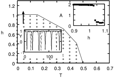
Figure 1: Phase diagram. $\left\langle L\right\rangle$ on the displayed curve satisfies $0.097<\left\langle L\right\rangle<0.107$. Inset: (right) Amplitude of oscillation A as a function of $h$. (left) Typical samples of the time evolution of $Y$ for $h=1.0$ (solid line), $h=1.02$ (dashed line), and $h=1.1$ (dotted line). Here, $T=0.05$ and $N=100$. The arrow represents the direction of the parameter change. $\left\langle L\right\rangle>0.1$ in the states where the symbols are placed.

The excitable nature of a system is characterized by the existence of spikes in a time series. Mathematically speaking, spikes are described by trajectories near a homoclinic orbit in a differential equation. As a simple example, let us consider an ordinary differential equation $\partial_{t}\phi=\omega-h\sin\phi$ for a phase variable $\phi\in[0,2\pi]$, in which there exists the homoclinic orbit when $\omega=h$. Then, when $h$ is slightly larger than $\omega$, a small perturbation for the fixed point $\phi_{*}=\sin^{-1}({\omega/h})$ yields one spike. On the other hand, when $h$ is slightly less than $\omega$, the system shows an array of spikes with a long interspike interval. The qualitative change in the trajectories is an example of saddle-node bifurcation. By using this simple dynamics as a model of excitable element, we study globally coupled excitable elements $\{\phi_{i}\}_{i=1}^{N}$ under the influence of noise Shinomoto :

$$\partial_{t}\phi_{i} =\omega-h\sin\phi_{i}-\frac{K}{N}\sum_{j=1}^{N}\sin(\phi_{i}-\phi_{j})+\xi_{i},$$ (1)

where $\xi_{i}(t)$ is Gaussian white noise that satisfies the relation $\left\langle\xi_{i}(t)\xi_{j}(t^{\prime})\right\rangle=2T\delta_{i,j}\delta(t-t^{\prime})$. Without loss of generality we can assume $K=1$, and we restrict our investigations to the case $\omega=1$. The control parameters are $h$ and $T$. All numerical results in this Letter have been calculated by employing an explicit discretization method with a time step $\delta t=0.05$.

The collective behavior of this system is described by the time evolution of a complex amplitude, which is given by

$$Z\equiv\frac{1}{N}\sum_{j=1}^{N}{\rm e}^{i\phi_{j}}.$$ (2)

In particular, for the expression $Z=X+iY$, where $X$ and $Y$ are real numbers, the expectation values of the angular momentum $L\equiv X(\partial_{t}Y)-(\partial_{t}X)Y$ are used to distinguish the oscillatory states ($\left\langle L\right\rangle\not=0$) from the stationary states ($\left\langle L\right\rangle=0$) Kuramoto3 . In Fig. 1, we show an approximate phase diagram in the form of a curve that satisfies the condition $0.097<\left\langle L\right\rangle<0.107$ in the parameter space $(T,h)$. A similar phase diagram was obtained in Ref. Shinomoto by measuring the frequency of the time-dependent phase distribution function. Here, the curve starting from $(T,h)\simeq(0,1)$ is related to a saddle-node bifurcation, while the curve from $(T,h)\simeq(0.5,0)$ is related to a Hopf bifurcation. It should be noted that a complicated bifurcation diagram appears near $T=0.1$, which originates from the Takens-Bogdanov type bifurcation Sakaguchi2 .

Preliminary:

In this study, we focus on systems near a saddle-node bifurcation. First, we fix $T=0.05$ and change $h$ across the bifurcation from below. Here, the amplitude of oscillation $A\equiv\left\langle[{\rm max}_{t}X(t)-{\rm min}_{t}X(t)]\right\rangle$ changes discontinuously at the bifurcation. (See inset of Fig. 1.) The discontinuous change in the amplitude is in a sharp contrast to a super-critical Hopf bifurcation at a collective level, where the amplitude of oscillation changes continuously at the bifurcation Kuramoto2 . It should be noted that in a manner similar to that of the critical phenomenon in equilibrium systems, the continuous transition leads to a critical divergence of amplitude fluctuation Daido . (See also Refs. Ritort ; Strogatz2 as reviews.) Thus, the discontinuous nature of the transition is not indicative of the appearance of critical phenomena.

Nevertheless, based on the fact that a typical time scale diverges at a saddle-node bifurcation, we take into account the fluctuation of interspike intervals. Explicitly, by using the phase of collective oscillation,

$$\theta\equiv{\rm arg}(Z),$$ (3)

we define the interspike interval $\hat{I}$ as the minimum time interval $[t,t+\hat{I}]$ over which the time integration of $\partial_{t}\theta$ is equal to $2\pi$ for a time $t$ satisfying $\theta(t)=-\pi/2$. As the most primitive statistical quantities of $\hat{I}$, we measured its average and fluctuation intensity defined by

$$I_{*}(h,N) \equiv\left\langle\hat{I}\right\rangle,$$ (4)

$$\chi(h,N) \equiv N\left(\left\langle\hat{I}^{2}\right\rangle-\left\langle\hat{I}\right\rangle^{2}\right).$$ (5)

In order to determine the divergent behaviors near the bifurcation in the thermodynamic limit, we performed finite-size scaling analysis by using systems with $N=10$, $100$, and $1000$. For each system, the values of $I_{*}(h,N)$ and $\chi(h,N)$ were calculated for several values of $h$. Then, we assume the scaling relations

$$I_{*}(h,N) \simeq N^{\frac{\zeta}{\nu}}F_{I}\left(\frac{h_{\rm c}-h}{h_{\rm c}}N^{\frac{1}{\nu}}\right),$$ (6)

$$\chi(h,N) \simeq N^{\frac{\gamma}{\nu}}F_{\chi}\left(\frac{h_{\rm c}-h}{h_{\rm c}}N^{\frac{1}{\nu}}\right),$$ (7)

where the exponents $\nu$, $\zeta$, and $\gamma$ and the critical value $h_{\rm c}$ are determined so that the scaling relations are valid. We also assume that a distribution function of $\hat{I}$ is expressed as a function of $\hat{I}N^{\zeta/\nu}$ when $h=h_{\rm c}$. By applying this assumption to $\chi(h,N)$ in (5), we find a relation $\gamma/\nu=2\zeta/\nu+1$, which yields

$$\nu=\gamma-2\zeta.$$ (8)

Moreover, since $I_{*}$ and $\chi$ are independent of $N$ in the regime $(h_{\rm c}-h)N^{1/\nu}\gg 1$, the asymptotic behaviors can be derived as $F_{I}(x)\simeq x^{-\zeta}$ and $F_{\chi}(x)\simeq x^{-\gamma}$. With the consideration of these conditions, we determine the values $h_{\rm c}=1.0283$, $\nu=3/2$, $\zeta=1/2$, and $\gamma=5/2$, for which the excellent collapses to universal curves are found, as displayed in Figs. 2 and 3.

Figure 2: $I_{*}N^{-1/3}$ as a function of $(1-h/h_{\rm c})N^{2/3}$. Here, $h_{\rm c}=1.0283$. The guide line represents a power-law function with exponent $-1/2$

Figure 3: $\chi N^{-3/2}$ as a function of $(1-h/h_{\rm c})N^{2/3}$. Here, $h_{\rm c}=1.0283$. The guide line represents a power-law function with exponent $-5/2$

Theory:

We now present a theory for the results $\zeta=1/2$ and $\gamma=5/2$. ($\nu$ is then determined from (8).) In the argument below, we assume that $\epsilon\equiv h_{\rm c}-h$ is a sufficiently small positive constant and consider the asymptotic limit $N\to\infty$ for the assumed value of $\epsilon$.

We first notice that for a sufficiently small value of $T$, the excitable elements are almost in synchronization. Thus, when setting $\phi_{i}=\theta+\delta\phi_{i}$, we assume that $|\delta\phi_{i}|\ll 1$. From this assumption and the definition of $\theta$ given in (3), we can derive the equation

$$\partial_{t}\theta=\omega-h\sin\theta+\eta,$$ (9)

with $\left\langle\eta(t)\eta(t^{\prime})\right\rangle=2(T/N)\delta(t-t^{\prime})$, where we have ignored the contribution of $O(\sum_{i=1}^{N}(\delta\phi_{i})^{2}/N)$ to the time evolution of $\theta$. Within this approximation, $h_{\rm c}$ is determined as $h_{\rm c}=\omega$. Although the equation we analyze has become quite simple, the calculation of the critical exponents is still non-trivial. By using a special technique, we can derive the distribution function of $\hat{I}$, from which we can calculate the values of the exponents Iwata2 . Since the calculation requires a complicated procedure, we present a method by which the values of the exponents can be determined without the distribution function of $\hat{I}$.

The basic idea of our analysis is to consider a distribution function of the average frequency $\hat{\Omega}$ over a time interval $\Delta t=MI_{*}$, where $M$ is a large number independent of $\epsilon$. (Note that $\Delta t$ depends on $\epsilon.)$ For the explicit expression

$$\hat{\Omega}=\frac{1}{\Delta t}\int_{0}^{\Delta t}dt(\partial_{t}\theta),$$ (10)

we can expect a large deviation property, which is given as

$$P(\hat{\Omega}=\Omega)\simeq{\rm e}^{-MNG(\Omega)/T},$$ (11)

where the rate function $G(\Omega)$ takes a minimum value zero when $\Omega=\Omega_{*}$. Then, it can be shown that $I_{*}$ in (4) is equal to $2\pi/\Omega_{*}$.

We now estimate the rate function $G(\Omega)$. Let $[\theta]$ be a trajectory $(\theta(t))_{t=0}^{\Delta t}$, and $\theta(0)$ is fixed as an arbitrary value. The probability density of trajectory is then expressed by

$${\cal P}([\theta])=\frac{1}{Z}{\rm e}^{-\frac{N}{4T}\int_{0}^{\Delta t}dt\left[(\partial_{t}\theta-f(\theta))^{2}+\frac{2T}{N}f^{\prime}(\theta)\right]},$$ (12)

where $f(\theta)=\omega-h\sin\theta$, the prime represents the derivative with respect to $\theta$, and $Z$ is a normalization factor. The last term corresponds to a Jacobian term associated with the transformation from a noise sequence $(\eta(t))_{t=0}^{\Delta t}$ to the trajectory $[\theta]$. By formally expressing $P(\hat{\Omega}=\Omega)$ as

$$P(\hat{\Omega}=\Omega)=\int{\cal D}[\theta]{\cal P}([\theta])\delta\left(\Omega-\frac{1}{\Delta t}\int_{0}^{\Delta t}dt(\partial_{t}\theta)\right),$$ (13)

we consider the trajectory whose weight becomes most dominant in the limit $N\to\infty$. The trajectory, which is denoted by $\theta^{\rm s}_{\Omega}$, is a periodic solution with period $2\pi/\Omega$ of the variational equation $\partial_{t}^{2}\theta(t)=-\partial_{\theta}U(\theta)/2$, where $U(\theta)=-f(\theta)^{2}$. The solution $\theta^{\rm s}_{\Omega}(t)$ is obtained from the energy conservation equation, which leads to the derivation of

$$\partial_{t}\theta^{\rm s}_{\Omega}=\sqrt{E(\Omega)-U(\theta^{\rm s}_{\Omega})},$$ (14)

where the parameter $E(\Omega)$ is related to the frequency $\Omega$ as

$$\frac{2\pi}{\Omega}=\int_{0}^{2\pi}\frac{d\theta}{\sqrt{E(\Omega)-U(\theta)}}.$$ (15)

Since $\theta^{\rm s}_{\Omega}$ contributes to $P(\hat{\Omega}=\Omega)$ much more than other $2\pi/\Omega$-periodic trajectories, it is reasonable to expect that $P(\hat{\Omega}=\Omega)\simeq{\cal P}([\theta^{\rm s}_{\Omega}])$. The substitution of (14) into (12) yields

$$G(\Omega)=\frac{I_{*}\Omega}{8\pi}\int_{0}^{2\pi}d\theta\frac{(\sqrt{E(\Omega)-U(\theta)}-\sqrt{-U(\theta)})^{2}}{\sqrt{E(\Omega)-U(\theta)}}.$$ (16)

It can be observed that $dG(\Omega)/d\Omega|_{\Omega_{*}}=0$ and $G(\Omega_{*})=0$ when $\Omega_{*}$ satisfies the condition $E(\Omega_{*})=0$. Therefore, the rate function $G(\Omega)$ takes a quadratic form

$$G(\Omega)=B(\epsilon)\Omega_{*}^{-4}(\Omega-\Omega_{*})^{2}$$ (17)

when $\Omega$ is close to $\Omega_{*}$, where $B(\epsilon)$ is calculated as

$$B(\epsilon)=\frac{8\sqrt{2}\pi}{3}\epsilon^{5/2}+O(\epsilon^{7/2}).$$ (18)

Furthermore, by considering (15) with $E=0$, we obtain

$$\Omega_{*}=\sqrt{2-\epsilon}\epsilon^{1/2}.$$ (19)

Now, we consider the average of $\hat{I}$ during the time interval $\Delta t$, which is denoted by $\hat{J}$. It can be easily confirmed that $\hat{J}=2\pi/\hat{\Omega}$. Then, by the transformation of the variable in (11) and (17), we derive

$$P(\hat{J}=J)\simeq{\rm e}^{-MNB(\epsilon)\left(J-2\pi/\Omega_{*}\right)^{2}/(4\pi^{2}T)}.$$ (20)

By substituting (18) and (19) into (20), we find that $\left\langle J\right\rangle\simeq\epsilon^{-1/2}$ and $\left\langle(J-\left\langle J\right\rangle)^{2}\right\rangle\simeq\epsilon^{-5/2}$. Since these $\epsilon$ dependences should be equal to those of $I_{*}$ and $\chi$, we arrive at the theoretical results $\zeta=1/2$ and $\gamma=5/2$. These values coincide perfectly with the numerical values.

Furthermore, our analysis yields a new formula for the phase diffusion constant $D$, which is expressed by $D\equiv\Delta t\left\langle(\hat{\Omega}-\Omega_{*})^{2}\right\rangle/2$ because $\hat{\Omega}=(\theta(\Delta t)-\theta(0))/\Delta t$. Indeed, from (11), we obtain

$$D=\frac{T}{2N}\frac{I_{*}}{G^{\prime\prime}(\Omega_{*})},$$ (21)

which leads to the power-law behavior $D=(3T/32\sqrt{2}\pi N)\epsilon^{-1}+O(\epsilon^{0})$. Here, with the crossover relation $\epsilon\simeq(N/T)^{-2/3}$, we conjecture $D\simeq(T/N)(N/T)^{2/3}$ at $\epsilon=0$, which was reported in Ref. Reimann .

Concluding remarks:

We have studied a simple model that exhibits critical behavior near a saddle-node bifurcation. The power-law divergence, $\chi\simeq\epsilon^{-5/2}$, which we have predicted for coupled excitable elements will be observed in experimental systems. Complicated systems such as those with a tactical network or integrate-and-fire dynamics will be analyzed by extending our theory.

The analysis of finite-dimensional systems is the next theoretical problem. As usual in critical phenomena, we wish to determine the upper-critical dimension above which the values of the exponents are the same as those in the globally coupled model. Then, we intend to develop a systematic method to take into account non-Gaussian fluctuations. The construction of such a theory is extremely interesting.

Before ending this Letter, let us recall that the amplitude of oscillation exhibits a discontinuous transition at the saddle-node bifurcation. Here, it should be noted that the co-existence of critical fluctuations with a discontinuous transition is one of the remarkable features of jamming transitions Fisher . This is not an accidental coincidence and can be explained in the following manner.

A standard characterization of the critical nature near a jamming transition is based on the nonlinear susceptibility $\chi_{4}(t)$, which quantifies the fluctuations of unlocking events during a time interval $t$ Onuki . Among the several theories for $\chi_{4}(t)$ Biroli ; Garrahan ; Miyazaki ; Iwata1 , one theory states that the divergence of $\chi_{4}(t)$ originates from the critical fluctuations of the time when an unlocking event occurs Iwata1 . By employing the method in Ref. Iwata1 , we can discuss the divergent behavior of amplitude fluctuations in the present problem. That is, the coexistence of a discontinuous transition and a critical fluctuation in coupled excitable elements can be described in a manner similar to that in jamming transitions.

Moreover, it has been recently shown that dynamical behaviors of the $k$-core percolation in a random graph exhibit a saddle-node bifurcation at the percolation point Iwata3 . Since it has been known that the $k$-core percolation is related to a kinetically constrained model and a random-field Ising model Duxbury ; Schwarz ; Toninelli ; Dhar ; Ohta , our work might be useful for theoretical analysis of such systems.

We hope that our theory of the nontrivial behavior of a simple model will stimulate further studies on subjects that increase the understanding of the cooperative nature of nonequilibrium systems.

The authors thank M. Iwata for discussions on related problems. This work was supported by a grant from the Ministry of Education, Science, Sports and Culture of Japan, No. 19540394.

References

- (1) R. Segev, M. Benveniste, E. Hulata, N. Cohen, A. Palevski, E. Kapon, Y. Shapira, and E. Ben-Jacob, Phys. Rev. Lett. 88, 118102 (2002).
- (2) J. M. Beggs and D. Plentz, J. Nerosci. 23, 11167 (2003).
- (3) E. Schneidman, M. J. Berry, R. Segev, and W. Bialek Nature 440, 1007 (2006).
- (4) C. Bedard, H. Kroger, and A. Destexhe, Phys. Rev. Lett. 97, 118102 (2006).
- (5) Y. F. Contoyiannis, F. K. Diakonos, C. Papaefthimiou, and G. Theophilidis, Phys. Rev. Lett. 93, 098101 (2004).
- (6) K. Kiyono, Z. R. Struzik, N. Aoyagi, F. Togo, and Y. Yamamoto, Phys. Rev. Lett. 95, 058101 (2005).
- (7) T. Yokogawa and T. Harada, arXiv:0708.2308.
- (8) H. Sakaguchi, Prog. Theor. Phys. 92, 1039 (1994).
- (9) C. W. Eurich, J. M. Herrmann, and U. A. Ernst, Phys. Rev. E 66, 066137 (2002).
- (10) C. Haldeman and J. M. Beggs, Phys. Rev. Lett. 94, 058101 (2005).
- (11) O. Kinouchi and M. Copelli, Nat. Phys. 2, 348 (2006).
- (12) A. Levina, J. M. Herrmann, and T. Geisel, Nat. Phys. 3, 857 (2007).
- (13) J. Teramae and T. Fukai, J. Comput. Neurosci. 22, 301 (2007).
- (14) M. A. Buice and J. D. Cowan, Phys. Rev. E 75, 051919 (2007).
- (15) G. L. Pellegrini, L. de Arcangelis, H. J. Herrmann, and C. Perrone-Capano, Phys. Rev. E 76, 016107 (2007).
- (16) S. Shinomoto and Y. Kuramoto, Prog. Theor. Phys. 75, 1105 (1986).
- (17) Y. Kuramoto, T. Aoyagi, I. Nishikawa, T. Chawanya, and K. Okuda, Prog. Theor. Phys. 87, 1119 (1992).
- (18) H. Sakaguchi, S. Shinomoto, and Y. Kuramoto, Prog. Theor. Phys. 79, 600 (1988).
- (19) Y. Kuramoto, Chemical Oscillations, Waves and Turbulence, (Springer, Berlin, 1984).
- (20) H. Daido, J. Stat. Phys. 60, 753 (1990).
- (21) S. H. Strogatz, Physica D 143, 1 (2000).
- (22) J. A. Acebron, L. L. Bonilla, C. J. Perez, F. Ritort, and R. Spigler, Rev. Mod. Phys. 77, 137 (2005).
- (23) M. Iwata and S. Sasa, in preperation
- (24) P. Reimann, C. Van den Broeck, H. Linke, P. Hanggi, J. M. Rubi, and A. Perez-Madrid, Phys. Rev. E 65, 031104 (2002).
- (25) C. Toninelli, G. Biroli, and D. S. Fisher, J. Stat. Phys. 120, 167 (2005).
- (26) R. Yamamoto and A. Onuki, Phys. Rev. E 58, 3515 (1998).
- (27) G. Biroli and J. P. Bouchaud, Europhys. Lett. 67, 21 (2004).
- (28) S. Whitelam, L. Berthier, and J. P. Garrahan, Phys. Rev. Lett. 92, 185705 (2004).
- (29) G. Biroli, J. P. Bouchaud, K. Miyazaki, and D. R. Reichman, Phys. Rev. Lett. 97, 195701 (2006).
- (30) M. Iwata and S. Sasa, Europhys. Lett. 77, 50008 (2007).
- (31) M. Iwata, G. Biroli, and S. Sasa, in preparation
- (32) M. Sellitto, G. Biroli, and C. Toninelli, Europhys. Lett. 69, 496 (2005).
- (33) J. M. Schwarz, A. J. Liu, and L. Q. Chayes, Europhys. Lett. 73, 560 (2006).
- (34) S. Sabhapandit, D. Dhar, and P. Shukla, Phys. Rev. Lett. 88, 197202 (2002).
- (35) C. L. Farrow, P. Shukla, and P. M. Duxbury, J. Phys. A. 40, 581 (2007).
- (36) H. Ohta and S. Sasa, Phys. Rev. E 77, 021119 (2008).