Multiband effects on the conductivity for a multiband Hubbard model

Abstract

The newly discovered iron-based superconductors have attracted lots of interests, and the corresponding theoretical studies suggest that the system should have six bands. In this paper, we study the multiband effects on the conductivity based on the exact solutions of one-dimensional two-band Hubbard model. We find that the orbital degree of freedom might enhance the critical value $U_{c}$ of on-site interaction of the transition from a metal to an insulator. This observation is helpful to understand why undoped High-$T_{c}$ superconductors are usually insulators, while recently discovered iron-based superconductors are metal. Our results imply that the orbital degree of freedom in the latter cases might play an essential role.

Recently discovered iron-based superconductors have attracted lots of experimental and theoretical interests s1 ; s2 ; s3 ; s4 ; s5 ; s6 ; s7 ; s8 ; s9 ; s10 ; s11 ; s12 ; s13 ; s14 ; s15 ; s16 ; s17 ; s18 . Despite the pairing mechanism being still controversial, a lot of theoretical works indicate that the orbital degeneracy may play a key role in these new family of high-Tc superconductors. Different from the conventional cuperate superconductors where the undoped compound is a Mott insulator, the pure LaOFeAs compound is a poor metal. This implies that the orbital degeneracy may dramatically affect the properties of the normal state. It is well known that one of the most basic model to understand the strongly correlated systems is the well-known single-band Hubbard model. Although thousands of works have been focused on such a deceptively simple model, the physical properties are not fully understood except the one-dimensional (1D) case where the exact solutions are available LiebW . The exact results indicate that the Hubbard model with a filling factor one is a Mott insulator at the zero temperature. It is quite interesting to ask whether the 1D Hubbard model with the same filling factor but with an additional orbital degree of freedom is still a Mott insulator in the zero temperature? Aiming to answer this problem, we study the conductivity of an extended 1D Hubbard model with the orbital degree of freedom in the scheme of the Bethe-ansatz solution. Unlike the single-band Hubbard model where the conductivity is found to be zero for any nonzero repulsive interactions, the Hubbard model with the orbital degree is found to be a conductor when the repulsive interaction is smaller than a critical value and a phase transition from metal to an insulator occurs when the on-site $U$ is larger than the critical value.

A 1D electronic system with the orbital degree of freedom can be modeled by

$$H=-t\sum_{i,a}\left(C_{i,a}^{+}C_{i+1,a}e^{i\phi/L}+h.c.\right)+U\sum_{i,a<a^{\prime}}n_{i,a}n_{i,a^{\prime}},$$ (1)

where $i=1,2,\dots,N$ identify the lattice site, $N$ is the total particle number, $L$ is the system-size, and $a=1,2,...,4$ labels the four states of single site, i.e. $\{1\uparrow,1\downarrow,2\uparrow,2\downarrow\}$ with $1,2$ being the indices of orbital and $\uparrow,\downarrow$ being the indices of spin LiMSZ98 ; LiGYE00 . The internal degree of freedom in the Hamiltonian (1) is specified to spin and orbital in present model. The $C^{+}_{ia}$ creates an electron with spin-orbital component $a$ on site $i$, and $n_{ia}:=C^{+}_{ia}C_{ia}$ is the corresponding number operator at site $i$. The system (1) is assumed with periodic boundary condition and $\phi$ is the magnetic flux piercing the ring. The system (1) is the Hamiltonian for four-component systems, and there are various discussions on multi-component Hubbard model in one dimension LiGYE00 ; Choy ; ChoyHaldane ; Schlottmann ; FrahmSS .

The conductivity of a many-body system generally takes the form

$$\sigma(\omega)=2\pi D_{c}\delta(\omega)+\sigma_{r}(\omega),$$ (2)

where $D_{c}$ is the charge stiffness and $\sigma_{r}(\omega)$ is the regular part of the conductivity. If $D_{c}$ is finite, the system is a perfect conductor; and if $D_{c}$ is zero but $\sigma_{r}(\omega)$ is finite, the system is a normal conductor; while if both of them are zero, the system is an insulator. At zero temperature, the transport properties of one-dimensional systems depend usually on the charge stiffness. Kohn showed that the charge stiffness can be computed from the ground-state energy $E(\phi)$ as Kohn64

$$D_{c}=\frac{N}{2}\frac{d^{2}E(\phi)}{d\phi^{2}},$$ (3)

where $\phi$ is the external magnetic flux. It is well-known that the magnetic flux $\phi$ piercing the system with the periodic boundary condition can be gauged out by imposing the twisted boundary conditions on the system su1 ; su2 . Therefore, solving the Schrodinger equation in the presence of the magnetic flux with periodic boundary condition is equivalent to that in the absence of the magnetic flux but with a twisted boundary condition for the wavefunctions

$$\psi(x_{1},\cdots,x_{i}+L,\cdots)=e^{i\phi}\psi(x_{1},\cdots,x_{i},\cdots).$$ (4)

We restrict our studies in the case of $L=N$. If $U=0$, the electrons do not interact with each other and the Hamiltonian can be transformed as

$$H=-2t\sum_{i,a}\cos(k+\phi/L)C_{k,a}^{+}C_{k,a}.$$

At the ground state, the electrons are arranged below the Fermi surface according to the Pauli exclusive principle. Then the density of electrons is

$$\frac{N}{L}=\frac{1}{2\pi}\int_{-k_{F}}^{k_{F}}4dk,$$

where $k_{F}$ is the Fermi momentum and

$$k_{F}=\frac{\pi N}{4L}.$$

For the case of $N=L$, the Fermi momentum is $k_{F}=\pi/4$. The ground-state energy is

$$\frac{E(\phi/L)}{L} = -\frac{4t}{\pi}\int_{-k_{F}}^{k_{F}}\cos(k+\phi/L)dk,$$ (5)

$$E(\phi/L) = -\frac{4tL}{\pi}\left[\sin(k_{F}+\phi/L)-\sin(-k_{F}+\phi/L)\right].$$ (6)

At the $U=0$ case, the ground-state charge stiffness can be obtained analytically as

$$D_{c}=\frac{2\sqrt{2}}{\pi}=0.9003163.$$

Therefore, the system is a perfect conductor. While if the interactions between the electrons tends to infinity, $U\rightarrow\infty$, each double occupation will cost an infinite energy thus the each site favors the single occupation. The system is an insulator. Therefore, a quantum phase transition from a conducting phase to an insulating phase should occur between these two limiting cases.

For finite $U$, the Hamiltonian is quasi-integrable if site occupations of more than two electrons are excluded. Physically, this is reasonable for the present studied case with filling factor one due to the state with more than two electrons on a site is energy unfavorable. Following the standard procedure Choy ; ChoyHaldane ; Schlottmann , the energy of the system (1) is

$$E(\phi)=-2t\sum_{j=1}^{N}\cos k_{j},$$ (7)

where the quasi-momentum $k_{j}$ should satisfy following Bethe-ansatz equations

$$e^{ik_{j}L} = e^{i\phi}\prod_{b=1}^{M}\frac{\sin k_{j}-\lambda_{b}+i\eta}{\sin k_{j}-\lambda_{b}-i\eta},$$

$$\prod_{l=1}^{N}\frac{\lambda_{a}-\sin k_{l}+i\eta}{\lambda_{a}-\sin k_{l}-i\eta} = -\prod_{b=1}^{M}\frac{\lambda_{a}-\lambda_{b}+i2\eta}{\lambda_{a}-\lambda_{b}-i2\eta}\prod_{c=1}^{M^{\prime}}\frac{\mu_{c}-\lambda_{a}+i\eta}{\mu_{c}-\lambda_{a}-i\eta},$$

$$\prod_{b=1}^{M}\frac{\mu_{a}-\lambda_{b}+i\eta}{\mu_{a}-\lambda_{b}-i\eta} = -\prod_{c=1}^{M^{\prime}}\frac{\mu_{a}-\mu_{c}+i2\eta}{\mu_{a}-\mu_{c}-i2\eta}\prod_{d=1}^{M^{\prime\prime}}\frac{\nu_{d}-\mu_{a}+i\eta}{\nu_{d}-\mu_{a}-i\eta},$$

$$\prod_{b=1}^{M^{\prime}}\frac{\nu_{a}-\mu_{b}+i\eta}{\nu_{a}-\mu_{b}-i\eta} = -\prod_{c=1}^{M^{\prime\prime}}\frac{\nu_{a}-\mu_{c}+i2\eta}{\nu_{a}-\mu_{c}-i2\eta},$$ (8)

where $\eta=U/4t$, $\lambda,\mu$ and $\nu$ are the rapidities.

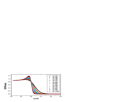
Figure 1: (color online). The curve of charge stiffness versus the on-site couplings for $L=N$. The cross point on $y$-axis is $2\sqrt{2}/\pi$.

For ground state (i.e., at zero temperature), the $k,\lambda,\mu,\nu$ are real roots of the Bethe ansatz equations (8). Taking the logarithm of the Bethe-ansatz equations, we get

$$2\pi I_{j} = k_{j}L+\phi+2\sum_{a}\tan^{-1}\left(\frac{\sin k_{j}-\lambda_{a}}{\eta}\right),$$

$$2\pi J_{a} = 2\sum_{l}\tan^{-1}\left(\frac{\lambda_{a}-\sin k_{l}}{\eta}\right)-2\sum_{b}\tan^{-1}\left(\frac{\lambda_{a}-\lambda_{b}}{2\eta}\right)$$

$$-2\sum_{c}\tan^{-1}\left(\frac{\mu_{c}-\lambda_{a}}{\eta}\right),$$

$$2\pi K_{a} = 2\sum_{b}\tan^{-1}\left(\frac{\mu_{a}-\lambda_{b}}{\eta}\right)-2\sum_{c}\tan^{-1}\left(\frac{\mu_{a}-\mu_{c}}{2\eta}\right)$$

$$-2\sum_{d}\tan^{-1}\left(\frac{\nu_{d}-\mu_{a}}{\eta}\right),$$

$$2\pi Q_{a} = 2\sum_{b}\tan^{-1}\left(\frac{\nu_{a}-\mu_{b}}{\eta}\right)-2\sum_{c}\tan^{-1}\left(\frac{\nu_{a}-\nu_{c}}{2\eta}\right),$$ (9)

where $\{I_{j},J_{a},K_{a},Q_{a}\}$ are quantum numbers. $I_{j}$ takes integer or half-odd integer depending on whether $M-1$ is odd or even. $J_{a},K_{a}$ and $Q_{a}$ take integer or half-odd integer depending on whether $N-M-M^{\prime}$, $M-M^{\prime}-M^{\prime\prime}$ and $M^{\prime}-M^{\prime\prime}$ are integer or half-odd integers, respectively. If $N=4n$ for $n$ being odd integer, the ground state is non-degenerate, and quantum number are centerred symmetrily around the zero point.

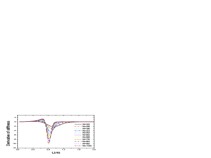
Figure 2: (color online). The derivative of the charge stiffness. At some certain coupling $U_{m}$, the derivative has a minimum.

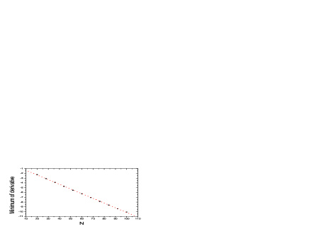
Figure 3: (color online). The curve of the minimum of derivative of the stiffness $D^{\prime}_{m}$ versus the system size $N$. The data can be fitted as $D^{\prime}_{m}=-0.374-0.098N$. One see that the minimum is divergence if the system size tends to infinity.

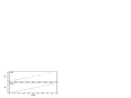
Figure 4: (color online). (a) The scaling behavior of the $U_{m}$. The data of the two-band model can be fitted as $U_{m}/4t=0.5475+1.19993/\ln N$. When the lattice number $N$ tends to infinity, $U_{m}$ becomes $U_{c}$, the critical value of $U_{c}/4t$ reads $0.548\pm 0.005$. (b) The same scaling analysis is performed for the single band Hubbard model. The data of the single band model can be fitted as $U_{m}/4t=0.00483+1.79084/\ln N$. The critical value of $U_{c}/4t$ reads $0.005\pm 0.006$, which covers the exact critical point $U_{c}=0$ of the single band Hubbard model.

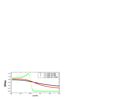
Figure 5: (color online). Charge stiffness with holes. Here the system size $L=100$ and the particle numbers $N=84,92,100$. The charge stiffness has a sharp peak only at the case of $L=N$.

We numerically solve the Bethe ansatz equations (9) with the finite system-size $L$. The charge stiffness versus the interaction $U$ is shown in Fig. 1. We see that the charge stiffness shows a sharp peak with the increasing system size. In the thermodynamic limit, the charge stiffness is expected as a step function, which takes a non-zero value at one side and zero at another side. The sudden jump point defines the critical $U_{c}$ of the phase transition. For the present model, if $U<U_{c}$, the system is a metal while if $U>U_{c}$, the system is an insulator. While for the single band Hubbard model, Lieb and Wu show that the Mott-insulator transition only happens at the $U_{c}=0$ case.

The critical $U_{c}$ can be determined by the derivative of the charge stiffness. The derivative of the charge stiffness versus the coupling $U$ is shown in Fig. 2. We see that the derivative has a minimum at a certain $U_{m}$. The minimum is decreasing with the increasing system-size. When the system-size tends to infinity, the minimum is divergent, which can be seen clearly in Fig. 3. From Fig. 3, the value of the minimum of derivative of the charge stiffness versus the system-size $N$ can be fitted into a straight line. Thus the charge stiffness becomes steeper and steeper as the system size increases.

The critical coupling $U_{m}$ with finite system-size versus the system-size is shown in Fig. 4. The data of $U_{m}$ and system-size $N(=L)$ can be fitted as $U_{m}/4t=0.5475+1.19993/\ln N$. When the system-size tends to infinity, $U_{m}$ becomes $U_{c}$. The critical $U_{c}/4t$ reads $0.548\pm 0.005$. We also perform the same scaling analysis for the single-band Hubbard model [Fig. 4(b)] and find that $U_{c}/4t=0.005\pm 0.006$. The difference between the two models is clear. For the case of $N=L$, the multiband might enhance the critical value $U_{c}/4t$.

Now we consider the system with some holes. For this case the Bethe ansatz solutions are solved by choosing suitable quantum numbers $\{I_{j},J_{a},K_{a},Q_{a}\}$. The charge stiffness versus the coupling $U$ is shown in Fig. 5, where the system-size is set to $L=100$ and particle numbers are $N=84,92,100$. We see that only at the case of $N=100$, the curve has a sharp transition; while for both cases $N=84$ and $N=92$, the charge stiffness always takes a nonzero value. This observation is consistent with the fact that the system would be a metal if we add some holes.

In conclusion, starting from the Bethe ansatz solutions of 1D two-band Hubbard model, we study the multiband effects on the conductivity. We find that multiband would enhance the critical value $U_{c}$ of on-site interactions of the transition from a metal to an insulator, while the critical $U_{c}$ for the single band Hubbard model is zero. The finite system-size would have a $1/\ln L$ correction to the actual value. The orbital degree of freedom might play an essential role in the properties of the electronic systems. These results are helpful to understand why undoped High-$T_{c}$ superconductors are usually insulators, while recently discovered iron-based superconductors are metal even without doping.

This work was supported by the Earmarked Grant for Research from the Research Grants Council of HKSAR, China (Projects No.HKU_3/05C), the national natural science foundation of China, and the national program for basic research of MOST. S. J. Gu is grateful for the hospitality of Institute of Physics at Chinese Academy Sciences.

References

- (1) Y. Kamihara, T. Watanabe, M. Hirano and H. Hosono, J. Am. Chem. Soc. 130, 3296 (2008).
- (2) D. J. Singh and M. H. Du, cond-mat/0803.0429.
- (3) K. Haule, J. H. Shim and G. Kotliar, cond-mat/0803.1279.
- (4) G. Xu, W. Ming, Y. Yao, X. Dai, S. Zhang and Z. Fang, con-mat/0803.1282.
- (5) C. Cao, P. J. Hirschfeld and H. P. Cheng, cond-mat/0803.3236.
- (6) X. H. Chen, T. Wu, G. Wu, R. H. Liu, H. Chen and D. F. Fang, cond-mat/0803.3603.
- (7) G. F. Chen, Z. Li, D. Wu, G. Li, W. Z. Hu, J. Dong, P. Zheng, J. L. Luo, N. L. Wang, cond-mat/0803.3790.
- (8) Z. A. Ren, et. al., Chin. Phys. Lett. 25, 2215 (2008) ; Z. A. Ren, et. al., Europhys. Lett., 82 (2008) 57002.
- (9) H. H. Wen, G. Mu, L. Fang, H. Yang and X. Zhu, Europhys. Lett. 82, 17009 (2008).
- (10) Z. A. Ren, G. C. Che, X. L. Dong, J. Yang, W. Lu, W. Yi, X. L. Shen, Z. C. Li, L. L. Sun, F. Zhou and Z. X. Zhao, cond-mat/0804.2582.
- (11) X. Dai, Z. Fang, Y. Zhou and F. C. Zhang, cond-mat/0803.3982.
- (12) P. A. Lee and X. G. Wen, cond-mat/0804.1739.
- (13) Q. M. Si and E. Abrahams, cond-mat/0804.2480.
- (14) S. Ishibashi, K. Terakura and H. Hosono, cond-mat/0804.2963.
- (15) F. Ma, Z. Y. Lu and T. Xiang, cond-mat/0804.3370.
- (16) Z. J. Yao, J. X. Li and Z. D. Wang, cond-mat/0804.4166.
- (17) X. L. Qi, S. Raghu, C. X. Liu, D. J. Scalapino and S. C. Zhang, cond-mat/0804.4332.
- (18) J. Li and Y. Wang, Chin. Phys. Lett. 25, 2232 (2008).
- (19) E. H. Lieb and F.Y. Wu, Phys. Rev. Lett. 25, 1445 (1968).
- (20) Y. Q. Li, M. Ma, D. N. Shi, and F. C. Zhang, Phys. Rev. Lett. 81, 3527 (1998).
- (21) Y. Q. Li, S. J. Gu, Z. J. Ying, and U. Eckern, Phys. Rev. B62, 4866 (2000).
- (22) T. C. Choy, Phys. Lett. 80 A, 49 (1980).
- (23) T. C. Choy and F. D. M. Haldane, Phys. Lett. A 90, 83 (1982).
- (24) P. Schlotmann, Phys. Rev. B43, 3101 (1991).
- (25) H. Frahm and A. Schadschneider, The Hubbard model: Its Physics and Mathematical Physics Eds. D. Baeriswyl et al., D. K. Campbell, J. M. P. Carmelo, F. Guinea, and E. Louis (Plenum Press, New York 1995) pp. 21; P. Schlottmann, Int. J. Mod. Phys. B 11, 355 (1997).
- (26) W. Kohn, Phys. Rev. 133, A171 (1964).
- (27) N. Byers and C.N. Yang, Phys. Rev. Lett. 7, 46 (1986).
- (28) B. S. Shastry and B. Sutherland, Phys. Rev. Lett. 65, 243 (1990).