1.0 in1.0 in1.25 in1.25 in

Estimation of Large Precision Matrices Through Block Penalization

This paper focuses on exploring the sparsity of the inverse covariance matrix $\boldsymbol{\Sigma}^{-1}$, or the precision matrix. We form blocks of parameters based on each off-diagonal band of the Cholesky factor from its modified Cholesky decomposition, and penalize each block of parameters using the $L_{2}$-norm instead of individual elements. We develop a one-step estimator, and prove an oracle property which consists of a notion of block sign-consistency and asymptotic normality. In particular, provided the initial estimator of the Cholesky factor is good enough and the true Cholesky has finite number of non-zero off-diagonal bands, oracle property holds for the one-step estimator even if $p_{n}\gg n$, and can even be as large as $\log p_{n}=o(n)$, where the data $\mathbf{y}$ has mean zero and tail probability $P(|y_{j}|>x)\leq K\exp(-Cx^{d})$, $d>0$, and $p_{n}$ is the number of variables. We also prove an operator norm convergence result, showing the cost of dimensionality is just $\log p_{n}$. The advantage of this method over banding by Bickel and Levina (2008) or nested LASSO by Levina et al. (2007) is that it allows for elimination of weaker signals that precede stronger ones in the Cholesky factor. A method for obtaining an initial estimator for the Cholesky factor is discussed, and a gradient projection algorithm is developed for calculating the one-step estimate. Simulation results are in favor of the newly proposed method and a set of real data is analyzed using the new procedure and the banding method.

Short Title: Block-penalized Precision Matrix Estimation.

AMS 2000 subject classifications. Primary 62F12; secondary 62H12.

Key words and phrases. Covariance matrix, high dimensionality, modified Cholesky decomposition, block penalty, block sign-consistency, oracle property.

1 Introduction

The need for estimating large covariance matrices arises naturally in many scientific applications. For example in bioinformatics, clustering of genes using genes expression data in a microarray experiment; or in finance, when seeking a mean-variance efficient portfolio from a universe of stocks. One common feature is that the dimension of the data $p_{n}$ is usually large compare with the sample size $n$, or even $p_{n}\gg n$ (genes expression data, fMRI data, financial data, among many others). The sample covariance matrix $\mathbf{S}$ is well-known to be ill-conditioned in such cases. Even for $\boldsymbol{\Sigma}=I$ the identity matrix, the eigenvalues of $\mathbf{S}$ are more spread out around 1 asymptotically as $p_{n}/n$ gets larger (the Marĉenko-Pastur law, Marĉenko and Pastur, 1967). It is singular when $p_{n}>n$, thus not allowing an estimate of the inverse of the covariance matrix, which is needed in many multivariate statistical procedures like the linear discriminant analysis (LDA), regression for multivariate normal data, Gaussian graphical models or portfolio allocations. Hence alternatives are needed for more accurate and useful estimation of covariance matrix.

One regularization approach is penalization, which is the main focus of this paper. Sparse estimation of the precision matrix $\boldsymbol{\Omega}=\boldsymbol{\Sigma}^{-1}$ has been investigated by many researchers, which is very useful in Gaussian graphical models or covariance selection for naturally ordered data (e.g. longitudinal data, see Diggle and Verbyla (1998)). Meinshausen and Bühlmann (2006) used the $L_{1}$-penalized likelihood to choose suitable neighborhood for a Gaussian graph and showed that $p_{n}$ can grow arbitrarily fast with $n$ for consistent estimation, while Li and Gui (2006) considered updating the off-diagonal elements of $\boldsymbol{\Omega}$ by penalizing on the negative gradient of the log-likelihood with respect to these elements. Banerjee, d’Aspremont and El Ghaoui (2006) and Yuan and Lin (2007) used $L_{1}$-penalty to directly penalize on the elements of $\boldsymbol{\Omega}$, and develop different semi-definite programming algorithms to achieve sparsity of the inverse. Friedman, Hastie and Tibshirani (2007) and Rothman et al. (2007) considered maximizing the $L_{1}$-penalized Gaussian log-likelihood on the off-diagonal elements of the precision matrix $\boldsymbol{\Omega}$, where the Graphical LASSO and the SPICE algorithms are proposed respectively in their papers for finding a solution, and the latter proved Frobenius and operator norms convergence results for the final estimators.

Pourahmadi (1999) proposed the modified Cholesky decomposition (MCD) which facilitates greatly the sparse estimation of $\boldsymbol{\Omega}$ through penalization. The idea is to decompose $\boldsymbol{\Sigma}$ such that for zero-mean data $\mathbf{y}=(y_{1},\cdots,y_{p_{n}})^{T}$, we have for $i=2,\cdots,p_{n}$,

$$y_{i}=\sum_{j=1}^{i-1}\phi_{i,j}y_{j}+\epsilon_{i},\text{ and }{\mathbf{T}}\boldsymbol{\Sigma}{\mathbf{T}}^{T}={\mathbf{D}},$$ (1.1)

where ${\mathbf{T}}$ is the unique unit lower triangular matrix with ones on its diagonal and $(i,j)^{\text{th}}$ element $-\phi_{i,j}$ for $j<i$, and ${\mathbf{D}}$ is diagonal with $i^{\text{th}}$ element $\sigma_{i}^{2}=\text{var}(\epsilon_{i})$. The optimization problem is unconstrained (since the $\phi_{ij}$’s are free variables), and the estimate for $\boldsymbol{\Omega}$ is always positive-definite. With MCD in (1.1), Huang et al. (2006) used the $L_{1}$-penalty on the $\phi_{i,j}$’s and optimized a penalized Gaussian log-likelihood through a proposed iterative scheme, with the case $p_{n}<n$ considered. Levina, Rothman and Zhu (2007) proposed a novel penalty called the nested LASSO to achieve a flexible banded structure of ${\mathbf{T}}$, and demonstrated by simulations that normality of data is not necessary, with $p_{n}>n$ considered.

For estimating the precision matrix $\boldsymbol{\Omega}$ for naturally ordered data, apart from the nested LASSO, Bickel and Levina (2008) proposed banding the Cholesky factor ${\mathbf{T}}$ in (1.1), with the banding order $k$ chosen by minimizing a resampling-based estimation of a suitable risk measure. The method works on estimating a covariance matrix as well. While these two methods are simple to use, they cannot eliminate blocks of weak signals in between stronger signals. For instance, consider a time series model

$$y_{i}=0.7y_{i-1}+0.3y_{i-3}+\epsilon_{i},$$

which corresponds to (1.1) with $\phi_{i,2}=0$, $\phi_{i,j}=0$ for $j\geq 4$. For example, this kind of model can arise in clinical trials data, where response on a drug for patients follows a certain kind of autoregressive process with weak signals preceding stronger ones. This implies a banded Cholesky factor ${\mathbf{T}}$, with the first and third off-diagonal bands being non-zero and zero otherwise. Banding and nested LASSO can band the Cholesky factor ${\mathbf{T}}$ starting from the fourth off-diagonal band, but cannot set the second off-diagonal band to zero. And if these methods choose to set the second off-diagonal band to zero, then the third non-zero off-diagonal band will be wrongly set to zero. Both failures can lead to inaccurate analysis or prediction, in particular the maximum eigenvalue of a precision matrix can then be estimated very wrongly. Clearly, an alternative method is required in this situation. We present the block penalization framework in the next section and more motivations and details of the methodology.

For more references, Smith and Kohn (2002) used a hierarchical Bayesian model to identify the zeros in the Cholesky factor ${\mathbf{T}}$ of the MCD. Fan, Fan and Lv (2007), using factor analysis, developed high-dimensional estimators for both $\boldsymbol{\Sigma}$ and $\boldsymbol{\Sigma}^{-1}$. Wu and Pourahmadi (2003) proposed a banded estimator through smoothing of the lower off-diagonal bands of $\hat{{\mathbf{T}}}$ obtained from the sample covariance matrix (implicitly, $p_{n}<n$). Then an order for banding of $\hat{{\mathbf{T}}}$ is chosen by using AIC penalty of normal likelihood of data. Furrer and Bengtsson (2007) considered gradually shrinking the off-diagonal bands’ elements of the sample covariance matrix towards zero. Bickel and Levina (2007) and El Karoui (2007) proposed the use of entry-wise thresholding to achieve sparsity in covariance matrices estimation, and proved various asymptotic results, while Rothman, Levina and Zhu (2008) generalizes these results to a class of shrinkage operators which includes many commonly used penalty functions. Wagaman and Levina (2007) developed an algorithm for finding a meaningful ordering of variables using a manifold projection technique called the Isomap, so that existing method like banding can be applied.

The rest of the paper is organized as follows. In section 2, we introduce the model for block penalization, and the motivation behind. A notion of sign-consistency, we name it block sign-consistency, is introduced. Together with asymptotic normality, we call it the oracle property of the resulting one-step estimator. An initial estimator needed for the one-step estimator, with the block zero-consistency concept, is introduced in section 2.5. A practical algorithm is discussed, with simulations and real data analysis in section 3. Theorems 2(i) and 3 are proved in the Appendix, whereas Theorems 2(ii) and 4 are proved in the Supplement.

2 Block Penalization Framework

2.1 Motivation

For data with a natural ordering of the variables, e.g. longitudinal data, or data with a metric equipped like spatial data with Euclidean distance, if data points are remote in time or space, they are likely to have weak or no correlation. Then ${\mathbf{T}}$ in equation (1.1), and thus $\boldsymbol{\Omega}$, are banded. Banding and nested LASSO mentioned in section 1 are based on this observation for obtaining a banded structure of the Cholesky factor ${\mathbf{T}}$. See Figure 1(b) for a picture of a banded Cholesky factor.

Also, for variables within a close neighborhood, the dependence structure should be similar. Equation (1.1) then says that coefficients on an off-diagonal band of the Cholesky factor ${\mathbf{T}}$ are close to neighboring coefficients (see also Wu and Pourahmadi (2003)). This means that we can improve our estimation if we can efficiently use neighborhood information (along an off-diagonal band of ${\mathbf{T}}$) to estimate the values of individual coefficients.

With these insights, we are motivated to use the block penalization method. In the context of wavelet coefficients estimation, Cai (1999) introduced a James-Stein shrinkage rule over a block of coefficients, whereas Antoniadis and Fan (2001, page 966) were the first to point out that such method can be regarded as a special kind of penalized likelihood which penalizes on the $L_{2}$ norm of a group of coefficients, and introduced a separable block-penalized least squares for simple solutions. Both papers argue that block thresholding helps pull information from neighboring empirical wavelet coefficients, thus increasing the information available for estimating coefficients within a block. Yuan and Lin (2006) introduced the same method, which they called the group LASSO, to select grouped variables (factors) in multi-factor ANOVA and compare grouped version of LARS and LASSO. Zhou, Rocha and Yu (2007) further introduced a penalty called the Composite Absolute Penalty (CAP) to introduce grouping and a hierarchy at the same time for the estimated parameters in a linear model.

Block penalization allows for a flexible banded structure in ${\mathbf{T}}$ since zero off-diagonal bands can precede the non-zero ones. This is an advantage over banding of Bickel and Levina (2008) and nested LASSO of Levina et al. (2007) as discussed in section 1. Moreover, the block sign-consistency property in Theorem 2(i) implies a banded estimated Cholesky factor ${\mathbf{T}}$ if the truth ${\mathbf{T}}_{0}$ is banded. See Figure 1 for a demonstration.

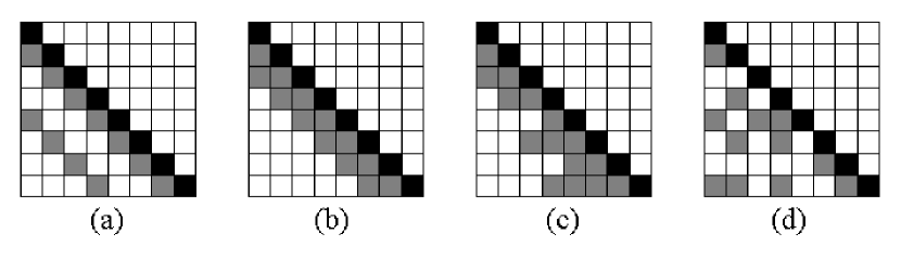
Figure 1: Pattern of zeros in the resulting estimator for ${\mathbf{T}}$ using (a)Block Penalization; (b)Banding; (c)Nested LASSO; (d)LASSO

2.2 Block penalization

As pointed out in Levina et al. (2007), the MCD in (1.1) does not require the normality assumption of the data, and they introduce a least squares version for their penalization. We also use such an approach, and define

$$L_{n}(\boldsymbol{\phi}_{n})=\sum_{i=1}^{n}\sum_{j=2}^{p_{n}}(y_{ij}-\mathbf{y}_{i[j]}^{T}\boldsymbol{\phi}_{j[j]})^{2},$$ (2.1)

with $\mathbf{y}_{i[j]}=(y_{i1},\cdots,y_{i,j-1})^{T}$, $\boldsymbol{\phi}_{n}=(\boldsymbol{\phi}_{2[2]}^{T},\cdots,\boldsymbol{\phi}_{p_{n}[p_{n}]}^{T})^{T}$, and $\boldsymbol{\phi}_{j[j]}=(\phi_{j,1},\cdots,\phi_{j,j-1})^{T}$.

When $p_{\lambda_{n}}(\cdot)$ is singular at the origin, the term-by-term penalty $\sum_{i=2}^{p_{n}}\sum_{j=1}^{i-1}p_{\lambda_{n}}(|\phi_{i,j}|)$ has its singularities located at each $\phi_{i,j}=0$, and the block penalty

$$J(\boldsymbol{\phi}_{n})=\sum_{j=1}^{p_{n}-1}p_{\lambda_{nj}}(\|\boldsymbol{\ell}_{j}\|),$$ (2.2)

has its singularities located at $\boldsymbol{\ell}_{j}=\mathbf{0}$ for $j=1,\cdots,p_{n}-1$, where $\lambda_{nj}=\lambda_{n}(p_{n}-j)^{1/2}$, $\boldsymbol{\ell}_{j}=(\phi_{j+1,1},\phi_{j+2,2},\cdots,\phi_{p_{n},p_{n}-j})^{T}$ is the $j^{th}$ off-diagonal band of the Cholesky factor ${\mathbf{T}}$ in (1.1), and $\|\cdot\|$ is the $L_{2}$ vector norm. Hence this block penalty either kills off a whole off-diagonal band $\boldsymbol{\ell}_{j}$ or keeps it entirely (see also Antoniadis and Fan (2001)).

Combining (2.1) and (2.2) is the block-penalized least squares

$$Q_{n}(\boldsymbol{\phi}_{n})=L_{n}(\boldsymbol{\phi}_{n})+nJ(\boldsymbol{\phi}_{n}).$$ (2.3)

We will use the SCAD penalty function for $p_{\lambda}(\cdot)$ in (2.2), defined through its derivative

$$p_{\lambda}^{\prime}(\theta)=\lambda\mathbf{1}_{\{\theta\leq\lambda\}}+(a\lambda-\theta)_{+}\mathbf{1}_{\{\theta>\lambda\}}.$$ (2.4)

SCAD penalty is an unbiased penalty function which has theoretical advantages over $L_{1}$-penalty (LASSO). See Lam and Fan (2007) for more details. In fact, in Fan, Feng and Wu (2007), the SCAD-penalized estimate of a graphical model is substantially sparser than the $L_{1}$-penalized one, which has spuriously large number of edges, partially due to the bias induced by $L_{1}$-penalty and hence requiring a smaller $\lambda$ that induces spurious edges. With $\boldsymbol{\hat{\phi}}_{n}$, we estimate ${\mathbf{D}}$ in (1.1) by

$$\hat{\sigma}_{1}^{2}=n^{-1}\sum_{i=1}^{n}y_{i1}^{2},\;\;\;\hat{\sigma}_{j}^{2}=n^{-1}\sum_{i=1}^{n}(y_{ij}-\mathbf{y}_{i[j]}^{T}\boldsymbol{\hat{\phi}}_{j[j]})^{2},\;\;\;j=2,3,\cdots,p_{n}.$$ (2.5)

2.3 Linearizing the SCAD penalty

Minimizing $Q_{n}(\boldsymbol{\phi}_{n})$ in (2.3) poses some challenges. Firstly, $Q_{n}(\boldsymbol{\phi}_{n})$ is not separable, which makes our problem computationally challenging. Secondly, the SCAD penalty complicates the computations as there are no easy simplifications of the problem like equation (5) in Antoniadis and Fan (2001, page 966).

Zou and Li (2007) showed that linearizing the SCAD penalty leads to efficient algorithms like the LARS to be applicable, and that sparseness, unbiasedness and continuity of the estimators continue to hold (see Fan and Li (2001)). Following their idea, we linearize each $p_{\lambda_{nj}}(\|\boldsymbol{\ell}_{j}\|)$ in (2.2) at an initial value $\|\boldsymbol{\ell}_{j}^{(0)}\|$ so that minimizing (2.3) is equivalent to minimizing, for $k=0$,

$$Q_{n}^{(k)}(\boldsymbol{\phi}_{n})=\sum_{i=1}^{n}\sum_{j=2}^{p_{n}}(y_{ij}-\mathbf{y}_{i[j]}^{T}\boldsymbol{\phi}_{j[j]})^{2}+n\sum_{j=1}^{p_{n}-1}p_{\lambda_{nj}}^{\prime}(\|\boldsymbol{\ell}_{j}^{(k)}\|)\|\boldsymbol{\ell}_{j}\|,$$ (2.6)

where we denote the resulting estimate by $\boldsymbol{\phi}_{n}^{(k+1)}$. Parallel to Theorem 1 and Proposition 1 of Zou and Li (2007), we state the following theorem concerning convergence in iterating (2.6) starting from $k=0$.

Theorem 1

For $k=0,1,2,\cdots$, the ascent property holds for $Q_{n}$ w.r.t. $\{\boldsymbol{\phi}_{n}^{(k)}\}$, i.e.

$$Q_{n}(\boldsymbol{\phi}_{n}^{(k+1)})\geq Q_{n}(\boldsymbol{\phi}_{n}^{(k)}).$$

Furthermore, let $\boldsymbol{\phi}_{n}^{(k+1)}=M(\boldsymbol{\phi}_{n}^{(k)})$, so that $M$ is the map carrying $\boldsymbol{\phi}_{n}^{(k)}$ to $\boldsymbol{\phi}_{n}^{(k+1)}$. If $Q_{n}(\boldsymbol{\phi}_{n})=Q_{n}(M(\boldsymbol{\phi}_{n}))$ only for stationary points of $Q_{n}$ and if $\boldsymbol{\phi}_{n}^{*}$ is a limit point of the sequence $\{\boldsymbol{\phi}_{n}^{(k)}\}$, then $\boldsymbol{\phi}_{n}^{*}$ is a stationary point $Q_{n}$.

This convergence result follows from more general convergence results for MM (minorize-maximize) algorithms. Hence starting from an initial value $\boldsymbol{\phi}_{n}^{(0)}$, we are able to iterate (2.6) to find a stationary point of $Q_{n}$. Note that even starting from the most primitive initial value $\boldsymbol{\phi}_{j[j]}=\mathbf{0}$, the first step gives a group LASSO estimator since $p_{\lambda_{nj}}^{\prime}(0)=\lambda_{nj}=\lambda_{n}(p_{n}-j)^{1/2}$. Hence the second step gives a biased reduced estimator of LASSO, as $p_{\lambda_{nj}}^{\prime}(\|\boldsymbol{\ell}_{j}^{(k)}\|)=0$ for $\|\boldsymbol{\ell}_{j}^{(k)}\|>a\lambda_{nj}$. In section 2.5 we show how to find a good initial estimator which is theoretically sound, and iterating until convergence is not always needed.

2.4 One-Step Estimator for $\boldsymbol{\phi}_{n}$

We now develop a one-step estimator to reduce the computational burden and prove that such an estimator enjoys the oracle property in Theorem 2. The performance of this one-step estimator depends on the initial estimator $\boldsymbol{\phi}_{n}^{(0)}$. Define, for $\boldsymbol{\ell}_{j0}$ denoting the true value of $\boldsymbol{\ell}_{j}$ in ${\mathbf{T}}$,

$$J_{n0}=\{j:\boldsymbol{\ell}_{j0}=\mathbf{0}\},\;\;\;J_{n1}=\{j:\boldsymbol{\ell}_{j0}\neq\mathbf{0}\}.$$

Definition 1

An initial estimator $\boldsymbol{\phi}_{n}^{(0)}$ is called block zero-consistent if there exists $\gamma_{n}=O(1)$ such that (a) $P\big{(}\max_{j\in J_{n0}}\|\boldsymbol{\ell}_{j}^{(0)}\|/(p_{n}-j)^{1/2}\geq\gamma_{n}\big{)}\rightarrow 0$ as $n\rightarrow\infty$, and (b) for the same $\gamma_{n}$, $P\big{(}\min_{j\in J_{n1}}\|\boldsymbol{\ell}_{j}^{(0)}\|/(p_{n}-j)^{1/2}\geq\gamma_{n}\big{)}\rightarrow 1.$

This definition is similar to the idea of zero-consistency introduced in Huang, Ma and Zhang (2006), but we now define it at the block level, which concerns the average magnitude of each element in the off-diagonal $\boldsymbol{\ell}_{j}^{(0)}$. With this, we present the main theorem of this section, the oracle property for the one-step estimator.

Theorem 2

Assume regularity conditions (A) - (E) in the Appendix, and the Cholesky factor ${\mathbf{T}}_{0}$ of the true precision matrix $\boldsymbol{\Omega}_{0}$ has $k_{n}<n$ non-zero off-diagonal bands. If the initial estimator $\boldsymbol{\phi}_{n}^{(0)}$ for $Q_{n}^{(0)}$ in (2.6) is block zero-consistent, then the resulting estimator $\boldsymbol{\hat{\phi}}_{n}$ by minimizing (2.6) satisfies the following:

• (Block sign-consistency) $P(A\cap B)\rightarrow 1$, where $A=\{\boldsymbol{\hat{\ell}}_{j}=\mathbf{0}\text{\emph{ for all }}j\in J_{n0}\},$ and $B=\{\text{\emph{sgn}}(\hat{\phi}_{j+k,k})=\text{\emph{sgn}}(\phi_{j+k,k}^{0})\text{\emph{ for all }}j\in J_{n1},\;k\text{\emph{ so that }}\phi_{j+k,k}^{0}\neq 0\}.$

• (Asymptotic normality) Let $\boldsymbol{\phi}_{n1}$ be the vector of elements of $\boldsymbol{\phi}_{n}$ corresponding to its non-zero off-diagonals. Then for a vector $\boldsymbol{\alpha}_{n}$ of the same size as $\boldsymbol{\hat{\phi}}_{n1}$ so that $\boldsymbol{\alpha}_{n}$ has at most $k_{n}$ non-zero elements and $\|\boldsymbol{\alpha}_{n}\|=1$, if $k_{n}^{4}(\log^{2}(k_{n}+1))^{4/d}/n=o(1)$, we have

  $$n^{1/2}(\boldsymbol{\alpha}_{n}^{T}\mathbf{H}_{n}\boldsymbol{\alpha}_{n})^{-1/2}\boldsymbol{\alpha}_{n}^{T}(\boldsymbol{\hat{\phi}}_{n1}-\boldsymbol{\phi}_{n1}^{0})\stackrel{{\scriptstyle\scriptscriptstyle\mathcal{D}}}{{\longrightarrow}}N(0,1),$$

where $\mathbf{H}_{n}$ is block diagonal with $p_{n}-1$ blocks. Its $(j-1)$-th block is $\sigma_{j0}^{2}\Sigma_{j11}^{-1}$, and $\Sigma_{j11}=E(\mathbf{y}_{i[j]}(1)\mathbf{y}_{i[j]}(1)^{T})$, where $\mathbf{y}_{i[j]}(1)$ contains the elements of $\mathbf{y}_{i[j]}$ corresponding to the non-zero off-diagonals’ elements of $\boldsymbol{\phi}_{j[j]}^{0}$.

From this theorem and regularity condition (C) in the Appendix, the size $p_{n}$ of the covariance matrix can be larger than $n$. In particular, if $k_{n}$ is finite, the oracle property still holds when $\log p_{n}=o(n)$. This is useful for many applications with $p_{n}>n$, when the sample covariance matrix becomes singular, whereas Theorem 3 shows that as long as the Cholesky factor is sparse enough, we can get an optimal estimator of the precision matrix via penalization.

Theorem 3

Let $\hat{{\mathbf{T}}}$ be the one-step estimator as in Theorem 2, and $\hat{{\mathbf{D}}}$ be diagonal with elements $\hat{\sigma}_{j}^{2}$ as defined in (2.5), so that $\hat{\boldsymbol{\Omega}}=\hat{{\mathbf{T}}}^{T}\hat{{\mathbf{D}}}^{-1}\hat{{\mathbf{T}}}$. Then under regularity conditions (A) - (E) in the Appendix, with $\boldsymbol{\Omega}_{0}$ denoting the true precision matrix,

$$\|\hat{\boldsymbol{\Omega}}-\boldsymbol{\Omega}_{0}\|_{\infty} =O_{P}((k_{n}+1)^{3/2}(\log p_{n}/n)^{1/2}),$$

$$\|\hat{\boldsymbol{\Omega}}-\boldsymbol{\Omega}_{0}\| =O_{P}((k_{n}+1)^{5/2}(\log p_{n}/n)^{1/2}),$$

where $\|M\|_{\infty}=\max_{i,j}|m_{i,j}|$, and $\|M\|=\lambda_{\max}^{1/2}(M^{T}M)$.

We will demonstrate related numerical results in section 3. From this theorem, the method of block penalization allows for consistent precision matrix estimation as long as the cost of dimensionality $\log p_{n}$ satisfies $(k_{n}+1)^{5}\log p_{n}/n=o(1)$. In particular, if $k_{n}$ is finite, we only need $\log p_{n}/n=o(1)$ for consistent estimation. On the other hand, provided the cost of dimensionality is not too large (e.g. $p_{n}=n^{a}$ for some $a>0$, so $\log p_{n}=a\log n$ and is negligible), we need $k_{n}=o(n^{1/3})$ for element-wise consistency.

2.5 Block zero-consistent initial estimator

We need a block zero-consistent initial estimator for finding an oracle one-step estimator in the sense of Theorem 2. The next theorem shows that the OLS estimator $\tilde{{\mathbf{T}}}$, where the sample covariance matrix is $\mathbf{S}=\tilde{{\mathbf{T}}}^{-1}\tilde{{\mathbf{D}}}(\tilde{{\mathbf{T}}}^{-1})^{T}$ using the MCD in (1.1), is block zero-consistent when $p_{n}/n\rightarrow\text{const.}<1$. When $p_{n}>n$, $\mathbf{S}$ is singular and $\tilde{{\mathbf{T}}}$ is not defined uniquely. Since we envisage a banded true Cholesky factor ${\mathbf{T}}_{0}$ with most non-zero off-diagonals close to the diagonal, we define $\tilde{{\mathbf{T}}}$ by considering the least square estimators of the regression

$$y_{i}=\sum_{j=c_{ni}}^{i-1}\phi_{i,j}y_{j}+\epsilon_{i},$$ (2.7)

where $c_{ni}=\max\{\lfloor i-\gamma n\rfloor,1\}$ with some constant $0<\gamma<1$ controlling the number of $y_{j}$’s on which $y_{i}$ regresses. The rest of the $\phi_{i,j}$’s are set to zero, recalling that even starting from the most primitive initial value $\boldsymbol{\phi}_{j[j]}=\mathbf{0}$, the one-step estimator is a group LASSO estimator since $p_{\lambda_{nj}}^{\prime}(0)=\lambda_{nj}=\lambda_{n}(p_{n}-j)^{1/2}$.

Theorem 4

Assume regularity conditions (A) to (E) in the Appendix. Then the estimator $\tilde{{\mathbf{T}}}$ obtained through the above series of regressions is block zero-consistent, provided all the true non-zero off-diagonal bands of ${\mathbf{T}}_{0}$ are within the first $\lfloor\gamma n\rfloor$ off-diagonal bands from the main diagonal of ${\mathbf{T}}_{0}$.

Remark : In high dimensional model selection, the condition of “irrepresentability” from Zhao and Yu (2006), “weak partial orthogonality” from Huang et al. (2006) or the UUP condition from Candès and Tao (2007) all describe the need of a weak association between the relevant covariates and the irrelevant ones under the true model, for the estimation procedures to pick up the correct sparse signals asymptotically. In our case, with (1.1) as the true model, the association between the variables $y_{i}$ and $y_{1},\cdots,y_{i-1}$ for $i=2,\cdots,p_{n}$ is incorporated into the tail assumption of the $y_{ij}$’s, which is specified in regularity condition (A). This assumption entails that the $|\phi_{i,j}|$’s for $i$ and $j$ far apart are small, so that the association between the relevant $y_{i}$’s (corr. to $\phi_{t,i}\neq 0$) and the irrelevant $y_{j}$’s (corr. to $\phi_{t,j}=0$) in model (1.1) are small.

In practice, for the series of regression described, we can continue to regress $y_{i}$ on the next $\lfloor\gamma n\rfloor$ $y_{j}$’s etc until all the $\tilde{\phi}_{i,j}$’s are obtained. We adapt this initial estimator in the numerical studies in section 3.

Also in practice, the rate at which $\max_{j\in J_{n0}}\|\boldsymbol{\ell}_{j}^{(0)}\|/(p_{n}-j)^{1/2}$ converges to zero in probability in definition 1 may not be fast enough for the OLS estimators. One way to improve the quality of the OLS estimators is to smooth along the off-diagonals of $\tilde{{\mathbf{T}}}$. For instance, Wu and Pourahmadi (2003) smoothed along off-diagonals of the OLS estimator $\tilde{{\mathbf{T}}}$ to reduce estimation errors. This amounts to assuming that the coefficients $\phi_{i,i-j}=f_{j,p_{n}}(i/p_{n})$, where $f_{j,p_{n}}(\cdot)$ is a smooth function defined on $[0,1]$. We then calculate the smoothed coefficients

$$\bar{\phi}_{j+k,k}=\sum_{r=1}^{p_{n}-j}w_{j}(r+j,k+j)\tilde{\phi}_{j+r,r},$$

where the weights $w_{j}(r+j,k+j)$ depends on the smoothing method. We use local polynomial smoothing with bandwidth $h\rightarrow\infty$ with $h/p_{n}\rightarrow 0$, so that $\text{var}(\bar{\phi}_{j+k,k})=O(n^{-1}h^{-1})$ (See Wu and Pourahmadi (2003) and Fan and Zhang (2000) for more details.).

2.6 Algorithm for practical implementation

Yuan and Lin (2006) proposed a group LASSO algorithm to solve problems similar to (2.6). However, when $p_{n}$ is large, the algorithm is computationally very expensive. Instead, we adapt an idea from Kim, Kim and Kim (2006) and use a gradient projection method to solve for the one-step estimator, which is computationally much less demanding. Since minimizing (2.6) can be considered as a weighted block-penalized least squares problem with weights $w_{nj}^{k}=np_{\lambda_{nj}}^{\prime}(\|\boldsymbol{\ell}_{j}^{(k)}\|)/\lambda_{n}$, it can be formulated as:

$$\text{minimizing }L_{n}(\boldsymbol{\phi}_{n})\text{ subject to }\sum_{j=1}^{s_{n}}w_{nj}^{k}\|\boldsymbol{\ell}_{j}\|\leq M$$ (2.8)

for some $M\geq 0$. Since the further off-diagonal bands of $\tilde{{\mathbf{T}}}$ are too short, in practice we stack them together until it is of length of order $p_{n}$. We then treat it as one block in the above dual-like problem, and denote by $s_{n}$ the number of off-diagonals in $\tilde{{\mathbf{T}}}$ after stacking.

Assume for now that all the tuning parameters are known. Starting from an initial value $\boldsymbol{\phi}_{n}^{(0)}$ and $t=1$, the gradient projection method involves computing the gradient $\nabla L_{n}(\boldsymbol{\phi}_{n}^{(t-1)})$ and defining $\mathbf{b}=\boldsymbol{\phi}_{n}^{(t-1)}-s\nabla L_{n}(\boldsymbol{\phi}_{n}^{(t-1)})$, where $s$ is the stepsize of iterations to be found in the next section. Denote by $\mathbf{b}_{(j)}$ the $j$th block of $\mathbf{b}$, with blocks formed according to the off-diagonals $\boldsymbol{\ell}_{j}$ of ${\mathbf{T}}$, $j=1,\cdots,s_{n}$. Then the main step of the algorithm is to solve

$$\boldsymbol{\phi}_{n}^{t}=\text{argmin}_{\boldsymbol{\phi}_{n}\in\mathcal{B}}\|\mathbf{b}-\boldsymbol{\phi}_{n}\|^{2},\;\;\text{ with }\;\;\mathcal{B}=\Big{\{}\sum_{j=1}^{s_{n}}w_{nj}^{k}\|\boldsymbol{\ell}_{j}\|\leq M\Big{\}},$$

which is called the projection step. It can be easily reformulated as solving

$$\min_{M_{j}}\sum_{j=1}^{s_{n}}(\|\mathbf{b}_{(j)}\|-M_{j})^{2}\text{ subject to }\sum_{j=1}^{s_{n}}w_{nj}^{k}M_{j}\leq M,\;\;M_{j}\geq 0,$$ (2.9)

where then $\boldsymbol{\ell}_{j}^{t}=M_{j}\mathbf{b}_{(j)}/\|\mathbf{b}_{(j)}\|$, and we iterate the above until convergence. Standard LARS or LASSO packages can solve (2.9) easily, but we adapt a projection algorithm by Kim et al. (2006) which can solve the above even faster. In solving (2.9), we are essentially projecting $(\|\mathbf{b}_{(1)}\|,\cdots,\|\mathbf{b}_{(s_{n})}\|)$ onto the hyperplane $\sum_{j=1}^{s_{n}}w_{nj}^{k}M_{j}=M$ with $M_{j}\geq 0$. The key observation is that if such projection has non-positive values on some $M_{j}$’s, then the solution to (2.9) should have those $M_{j}$’s exactly equal zero. Hence we can then recalculate the projection onto the reduced hyperplane until no more negative values occur in the projection, and it is easy to see that at most $s_{n}$ such iterations are needed to solve (2.9). In detail, we start at $\tau=\{1,\cdots,s_{n}\}$, and calculate the projection

$$M_{j}=\mathbf{1}_{\{j\in\tau\}}\Big{[}\|\mathbf{b}_{(j)}\|+\Big{(}M-\sum_{r\in\tau}w_{nr}^{k}\|\mathbf{b}_{(r)}\|\Big{)}w_{nj}^{k}/\sum_{r\in\tau}(w_{nr}^{k})^{2}\Big{]}$$ (2.10)

for $j=1,\cdots,s_{n}$. We then update $\tau=\{j:M_{j}>0\}$ and calculate the above projection again until $M_{j}\geq 0$ for all $j$.

2.7 Choice of tuning parameters

There are three tuning parameters introduced in the previous section, namely $\lambda_{n}$, $M$ and $s$. The small number $s$ is a parameter for the gradient projection algorithm and it is required that $s<2/L$, where $L$ is the Lipchitz constant of the gradient of $L_{n}(\boldsymbol{\phi}_{n})$. It can be easily shown that $L=2\lambda_{\max}^{1/2}(S_{Y}^{2})$, where $S_{Y}=\text{diag}(\sum_{i=1}^{n}\mathbf{y}_{i[2]}\mathbf{y}_{i[2]}^{T},\cdots,\sum_{i=1}^{n}\mathbf{y}_{i[p_{n}]}\mathbf{y}_{i[p_{n}]}^{T})$, so that $s<\lambda_{\max}^{-1/2}(S_{Y}^{2})$.

For the choice of $M$, note that for a suitable $\lambda_{n}$ and that $\boldsymbol{\ell}_{j}=\boldsymbol{\ell}_{j0}$ in (2.8), we either have $w_{nj}^{k}=0$ or $\boldsymbol{\ell}_{j0}=\mathbf{0}$. Thus, the value of $\sum_{j=1}^{s_{n}}w_{nj}^{k}\|\boldsymbol{\ell}_{j0}\|$ is always zero. In view of this, the oracle choice of $M$ is actually zero. We adapt this choice in the numerical studies in section 3.

For the choice of $\lambda_{n}$, we use a GCV criterion similar to the one used by Kim et al. (2006). We find $\tilde{{\mathbf{T}}}$ as defined in section 2.5, and smooth the off-diagonal bands of $\tilde{{\mathbf{T}}}$ to form $\bar{{\mathbf{T}}}$. Define $\mathbf{W}_{j}=\text{diag}(w_{ns_{n}}^{k}/\|\bar{\boldsymbol{\ell}}_{s_{n}}\|\mathbf{1}_{j-s_{n}}^{T},w_{n(c_{nj}-1)}^{k}/\|\bar{\boldsymbol{\ell}}_{c_{nj}-1}\|,\cdots,w_{n2}^{k}/\|\bar{\boldsymbol{\ell}}_{2}\|,w_{n1}^{k}/\|\bar{\boldsymbol{\ell}}_{1}\|)$ and ${\mathbf{X}}_{j}=(\mathbf{y}_{1[j]},\mathbf{y}_{2[j]},\cdots,\mathbf{y}_{n[j]})^{T}$, where $\mathbf{1}_{m}$ denote the column vector of ones of length $m$. The GCV-type criterion is to minimize

$$\text{GCV}(\lambda_{n})=\sum_{j=2}^{p_{n}}\frac{n\sum_{i=1}^{n}(y_{ij}-\mathbf{y}_{i[j]}^{T}\bar{\boldsymbol{\phi}}_{j[j]})^{2}}{(n-\text{tr}[{\mathbf{X}}_{j}({\mathbf{X}}_{j}^{T}{\mathbf{X}}_{j}+\lambda_{n}\mathbf{W}_{j})^{-1}{\mathbf{X}}_{j}^{T}])^{2}},$$ (2.11)

where $\text{tr}(\cdot)$ denotes the trace of a square matrix. In practice we calculate GCV($\lambda_{n}$) on a grid of values of $\lambda_{n}$ and find the one that minimizes GCV($\lambda_{n}$) as the solution.

3 Simulations and Data Analysis

In this section, we compare the performance of block penalization (BP) to other regularization methods, in particular banding of Bickel and Levina (2008) and LASSO of Huang et al. (2006).

For measuring performance, the Kullback-Leibler loss for a precision matrix is used. It has been used in Levina et al. (2007), defined as

$$L_{KL}(\boldsymbol{\Sigma},\hat{\boldsymbol{\Sigma}})=\text{tr}(\hat{\boldsymbol{\Sigma}}^{-1}\boldsymbol{\Sigma})-\log|\hat{\boldsymbol{\Sigma}}^{-1}\boldsymbol{\Sigma}|-p_{n},$$

which is the entropy loss but with the role of covariance matrix and its inverse switched. See Levina et al. (2007) for more details of the loss function. We also evaluate the operator norm $\|\hat{\boldsymbol{\Omega}}-\boldsymbol{\Omega}_{0}\|$ for different methods to illustrate the results in Theorem 3 in our simulation studies. The proportions of correct zeros and non-zeros in the estimators for the Cholesky factors are reported.

3.1 Simulation analysis

The following three covariance matrices are considered in our simulation studies.

• $\boldsymbol{\Sigma}_{1}=0.8I$.

• $\boldsymbol{\Sigma}_{2}:\phi_{i,i-1}=\phi_{i,i-2}=-0.6,\;\phi_{i,i-4}=\phi_{i,i-6}=-0.4$, $\phi_{i,j}=0$ otherwise; $\sigma_{j0}^{2}=0.8$.

• $\boldsymbol{\Sigma}_{3}:\phi_{i,j}=0.5^{i-j},j<i$; $\sigma_{j0}^{2}=0.1$.

The covariance matrix $\boldsymbol{\Sigma}_{1}$ is a constant multiple of the identity matrix, which is considered by Huang et al. (2006) and Levina et al. (2007). $\boldsymbol{\Sigma}_{2}$ is the covariance matrix of an AR(6) process, which has a banded inverse. $\boldsymbol{\Sigma}_{3}$ is the covariance matrix of an MA(1) process. It is itself tri-diagonal and has a non-sparse inverse. We investigate the performance of BP in such a non-sparse case.

Regularity conditions (B) to (E) are satisfied for the three models by construction. Since all three define stationary time series models in the sense of (1.1), condition (A) is satisfied from Gaussian to general Weibull-distributed innovations.

We generated $n=100$ observations for each simulation run, and considered $p_{n}=50,100$ and $200$. We used $N=50$ simulation runs throughout. In order to illustrate theoretical results and test the robustness of the BP method on heavy-tailed data, on top of multivariate normal for the variables, we also consider the multivariate $t_{3}$ for the variables, which violated condition (A). Tuning parameters for the LASSO and banding are computed using 5-fold CV, while the parameter $\lambda_{n}$ for the BP is obtained by minimizing GCV$(\lambda_{n})$ in (2.11). We set the smoothing parameter $h=0.3$ for local linear smoothing along the off-diagonal bands for demonstration purpose. The constant $\gamma$ and stacking parameter $s_{n}$ mentioned in section 2.5 are set at 0.9 and $p_{n}-\lceil 2p_{n}^{1/2}\rceil$ respectively. In fact we have done simulations (not shown) showing that smoothing along off-diagonals for the initial estimator can improve the performance of the one-step estimator. All the results below for the performance of BP are based on such smoothed initial estimators. Also, all subsequent tables show the median of the 50 simulation runs, and the number in the bracket is the $\text{SD}_{\text{mad}}$ which is a robust estimate of the standard deviation, defined by the interquartile range divided by 1.349.

Not shown here, we have carried out comparisons between using GCV-based and 5-fold CV-based tuning parameter $\lambda_{n}$ for the BP method, and both performed similarly. However, the GCV-based method is much quicker, and hence results of simulations are presented with the GCV-based BP method only.

Table 1: Kullback-Leibler loss for multivariate normal and $t_{3}$ simulations.

		Multivariate normal			Multivariate $t_{3}$
	$p_{n}$	LASSO	Banding	BP	LASSO	Banding	BP
$\boldsymbol{\Sigma}_{1}$	100	1.0(.1)	1.1(.8)	1.0(.1)	7.7(3.8)	10.7(9.3)	7.8(3.9)
	200	2.1(.2)	2.4(3.4)	2.1(.2)	16.4(9.7)	22.9(18.8)	16.4(9.7)
$\boldsymbol{\Sigma}_{2}$	100	27.2(1.4)	11.1(6.5)	5.6(.5)	110.7(29.2)	57.7(21.1)	28.2(10.6)
	200	264.6(39.9)	20.4(12.3)	11.5(.7)	789.5(132.0)	101.6(36.0)	54.7(14.2)
$\boldsymbol{\Sigma}_{3}$	100	8.8(.7)	7.8(9.7)	4.3(2.0)	40.2(7.6)	31.8(14.9)	19.8(7.9)
	200	19.4(1.5)	24.9(83.4)	18.1(23.1)	99.6(23.6)	70.3(35.4)	56.3(26.0)

Table LABEL:table:2 shows the Kullback-Leibler loss from various methods for multivariate normal and $t_{3}$ simulations. We omit the case for $p_{n}=50$ to save space, but results are similar to those for higher dimensions. In general the higher the dimension, the larger the loss is for all the methods. On $\boldsymbol{\Sigma}_{1}$, all methods perform similarly as expected (sample covariance matrix performs much worse and is not shown). However on $\boldsymbol{\Sigma}_{2}$, BP performs much better for all $p_{n}$ considered, especially when multivariate $t_{3}$ is concerned. The better performance is expected, since BP can eliminate weaker signals that precede stronger ones, but not particularly so for other methods. On $\boldsymbol{\Sigma}_{3}$, BP performs slightly better on average, particularly for multivariate $t_{3}$ simulations. For normal data, LASSO has smaller variability, though.

Table 2: Operator norm of difference $\|\hat{\boldsymbol{\Omega}}-\boldsymbol{\Omega}_{0}\|$ for different methods.

		Multivariate normal			Multivariate $t_{3}$
	$p_{n}$	LASSO	Banding	BP	LASSO	Banding	BP
$\boldsymbol{\Sigma}_{1}$	100	.6(.1)	.7(.3)	.6(.1)	1.7(.5)	2.0(.8)	1.7(.5)
	200	.7(.1)	.8(.4)	.7(.1)	1.8(.6)	2.0(.9)	1.8(.5)
$\boldsymbol{\Sigma}_{2}$	100	5.9(.4)	6.2(3.5)	2.5(.4)	11.3(4.6)	11.0(6.6)	7.2(3.5)
	200	29.1(11.3)	5.7(3.4)	2.6(.4)	58.1(11.2)	12.1(5.7)	7.7(2.3)
$\boldsymbol{\Sigma}_{3}$	100	14.7(1.6)	19.0(14.2)	11.6(1.9)	40.3(9.1)	33.8(13.5)	28.1(6.6)
	200	16.0(1.4)	27.4(63.7)	18.4(6.1)	46.1(6.0)	42.2(17.3)	35.5(11.0)

To demonstrate results of Theorem 3, the operator norm of difference $\|\hat{\boldsymbol{\Omega}}-\boldsymbol{\Omega}_{0}\|$ for different methods are summarized in Table LABEL:table:4. Clearly BP performs better in comparison with LASSO and banding on $\boldsymbol{\Sigma}_{2}$, in both normal and $t_{3}$ innovations. The performance gap gets larger as $p_{n}$ increases. For $\boldsymbol{\Sigma}_{3}$ BP still outperforms the other two methods in general, especially for heavy-tailed data.

Table 3: Correct zeros and non-zeros(%) in the estimated Cholesky factors for $\boldsymbol{\Sigma}_{2}$.

		Multivariate normal			Multivariate $t_{3}$
	$p_{n}$	LASSO	Banding	BP	LASSO	Banding	BP
Correct	50	60.6(2.3)	73.5(20.1)	100(0)	56.5(3.5)	89.1(12.3)	95.6(14.0)
percentage	100	75.3(.9)	87.7(12.0)	100(0)	70.5(2.6)	94.4(5.8)	100(0)
of zeros	200	73.5(.7)	92.9(8.7)	100(0)	72.0(.7)	97.3(2.7)	100(0)
Correct	50	99.6(.4)	100(0)	100(0)	96.4(1.6)	71.3(35.0)	100(0)
percentage	100	99.2(.3)	100(0)	100(0)	95.1(1.8)	72.3(33.3)	100(0)
of non-zeros	200	99.3(.3)	100(0)	100(0)	97.1(.7)	80.5(25.9)	100(0)

Finally, to illustrate the ability to capture sparsity, we focus on $\boldsymbol{\Sigma}_{2}$ and summarize the correct percentages of zeros and non-zeros estimated in Table LABEL:table:5. BP almost gets all the zeros and non-zeros right in all simulations. The LASSO does poorly in the correct percentages of zeros. This is due to biases induced by LASSO that require a relatively small $\lambda$, resulting in many spurious non-zero coefficients. The banding method does not work well too. However, note that both banding and BP do better as dimension increases.

3.2 Real data analysis

We analyze the call center data using the BP method. This set of data is described in detail and analyzed by Shen and Huang (2005), and we thank you for the data courtesy by the authors.

The original data consists of details of every call to a call center of a major northeastern U.S. financial firm in 2002. Removing calls from weekends, holidays, and days when recording equipment was faulty, we obtain data from 239 days. On each of these days, the call center open from 7am to midnight, so there is a 17-hour period for calls each day. For ease of comparison, following Huang et al. (2006) and Bickel and Levina (2008), we use the data which is divided into 10-minute intervals, and the number of calls in each interval is denoted by $N_{ij}$, for days $i=1,\cdots,239$ and interval $j=1,\cdots,102$. The transformation $y_{ij}=(N_{ij}+1/4)^{1/2}$ is used to make the data closer to normal.

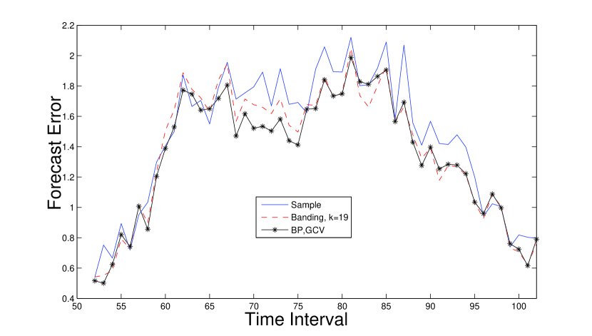
Figure 2: Mean absolute forecast errors for different estimation methods. Average is taken over 34 days of test data from November to December, 2002.

The goal is to forecast the counts of arrival calls in the second half of the day from those in the first half of the day. If we assume $\mathbf{y}_{i}=(y_{i1},\cdots,y_{i,102})^{T}\sim N(\boldsymbol{\mu},\boldsymbol{\Sigma})$, partitioning $\mathbf{y}_{i}$ into $\mathbf{y}_{i}^{(1)}$ and $\mathbf{y}_{i}^{(2)}$ where $\mathbf{y}_{i}^{(1)}=(y_{i1},\cdots,y_{i,51})^{T},\mathbf{y}_{i}^{(2)}=(y_{i,52},\cdots,y_{i,102})^{T}$, and denoting

$$\boldsymbol{\mu}=\left(\begin{array}[]{c}\boldsymbol{\mu}_{1}\\ \boldsymbol{\mu}_{2}\\ \end{array}\right),\;\;\boldsymbol{\Sigma}=\left(\begin{array}[]{cc}\boldsymbol{\Sigma}_{11}\;\;\boldsymbol{\Sigma}_{12}\\ \boldsymbol{\Sigma}_{21}\;\;\boldsymbol{\Sigma}_{22}\\ \end{array}\right),$$

the best mean square error forecast is then given by the conditional mean

$$\hat{\mathbf{y}}^{(2)}=E(\mathbf{y}^{(2)}|\mathbf{y}^{(1)})=\hat{\boldsymbol{\mu}}_{2}+\hat{\boldsymbol{\Sigma}}_{21}\hat{\boldsymbol{\Sigma}}_{11}^{-1}(\mathbf{y}^{(1)}-\hat{\boldsymbol{\mu}}_{1}).$$

This is also the best mean square error linear predictor without normality assumption.

To compare performance of different estimators of $\boldsymbol{\Sigma}$, we divide the data into a training set (Jan. to Oct., 205 days) and a test set (Nov. and Dec., 34 days). We estimate $\hat{\boldsymbol{\mu}}=\sum_{i=1}^{205}\mathbf{y}_{i}/205$, and $\hat{\boldsymbol{\Sigma}}$ by sample covariance, banding and BP. For each time interval $j=52,\cdots,102$, we consider the mean absolute forecast error

$$\text{Err}_{j}=\frac{1}{34}\sum_{i=206}^{239}|\hat{y}_{ij}-y_{ij}|.$$

For BP, we use GCV with $h=0.1$. The number $k=19$ for banding is used in Bickel and Levina (2008). From Figure 2, it is clear that the BP outperforms the other two methods, in particular for the time intervals 66 to 75 corresponding to the mid-afternoon.

Appendix: Proof of Theorems 2(i) and 3

We state the following general regularity conditions for the results in section 2.

• The data $\mathbf{y}_{i},i=1,2,\cdots,n$ are i.i.d. with mean zero and variance $\boldsymbol{\Sigma}_{0}$, a symmetric positive-definite matrix of size $p_{n}$. The tail probability of $\mathbf{y}_{i}$ satisfies, for $j=1,2,\cdots,p_{n}$, $P(|y_{ij}|>x)\leq K\exp(-Cx^{d})$, where $d>0$ and $C$, $K$ are constants. The innovations $\epsilon_{i2},\cdots,\epsilon_{ip_{n}}$ for $i=1,\cdots,n$ in (1.1) are mutually independent zero-mean r.v.’s and $\text{var}(\epsilon_{ij})=\sigma_{j0}^{2}$, having tail probability bounds similar to the $y_{ij}$’s.

• The variance-covariance matrix $\boldsymbol{\Sigma}_{0}$ in (A) has eigenvalues uniformly bounded away from 0 and $\infty$ w.r.t. $n$. That is, there exists constants $C_{1}$ and $C_{2}$ such that

  $$0<C_{1}<\lambda_{\min}(\boldsymbol{\Sigma}_{0})\leq\lambda_{\max}(\boldsymbol{\Sigma}_{0})<C_{2}<\infty\;\;\;\text{for all }n,$$

  where $\lambda_{\min}(\boldsymbol{\Sigma}_{0})$ and $\lambda_{\max}(\boldsymbol{\Sigma}_{0})$ are the minimum and maximum eigenvalues of $\boldsymbol{\Sigma}_{0}$ respectively.

• Let $d_{n1}=\min\{\phi_{n1j}^{0}:\phi_{n1j}^{0}>0\}$, where $\phi_{n1j}^{0}$ is the $j$-th element of $\boldsymbol{\phi}_{n1}^{0}$ (see Step 2.1 in the proof of Theorem 2(i) for a definition). Then as $n\rightarrow\infty$,

  $$\frac{k_{n}\log p_{n}}{nd_{n1}^{2}}\rightarrow 0,\quad\frac{k_{n}^{2}\log p_{n}}{n\lambda_{n}}\rightarrow 0,\quad\frac{\log p_{n}}{n\lambda_{n}^{2}}\rightarrow 0.$$

• The tuning parameter $\lambda_{n}$ satisfies

  $$0<\lambda_{n}<\min_{j\in J_{n1}}\frac{\|\boldsymbol{\ell}_{j0}\|}{a(p_{n}-j)^{1/2}},$$

  with $(p_{n}-j)\rightarrow\infty$ for all $j\in J_{n1}$ as $n\rightarrow\infty$.

• The values $\sigma_{\epsilon M}^{2}=\max_{1\leq t\leq p_{n}}\sigma_{t0}^{2}$ and $\sigma_{yM}^{2}=\max_{1\leq r\leq p_{n}}\text{var}(y_{jr})$ are bounded uniformly away from zero and infinity.

The following lemma is a direct consequence of Theorem 5.11 of Bai and Silverstein (2006).

Lemma 1

Let $\{\mathbf{y}_{i}\}_{1\leq i\leq n}$ be a random sample of $n$ vectors with length $q_{n}$, each with mean $\mathbf{0}$ and covariance matrix $\boldsymbol{\Sigma}$. In addition, each element of $\mathbf{y}_{i}$ has finite fourth moment. Then if $q_{n}/n\rightarrow\ell<1$, the sample covariance matrix $\mathbf{S}_{n}=n^{-1}\sum_{i=1}^{n}\mathbf{y}_{i}\mathbf{y}_{i}^{T}$ satisfies, almost surely,

$$\lim_{n\rightarrow\infty}\lambda_{\max}(\mathbf{S}_{n})\leq\lambda_{\max}(\boldsymbol{\Sigma})(1+\sqrt{\ell})^{2},\;\;\lim_{n\rightarrow\infty}\lambda_{\min}(\mathbf{S}_{n})\geq\lambda_{\min}(\boldsymbol{\Sigma})(1-\sqrt{\ell})^{2}.$$

Proof of Lemma 1. By Theorem 5.11 of Bai and Silverstein (2006), the matrix $\mathbf{S}_{n}^{*}=\boldsymbol{\Sigma}^{-1/2}\mathbf{S}_{n}\boldsymbol{\Sigma}^{-1/2}$ which is the sample covariance matrix of $\boldsymbol{\Sigma}^{-1/2}\mathbf{y}_{i}$, has

$$\lim_{n\rightarrow\infty}\lambda_{\max}(\mathbf{S}_{n}^{*})=(1+\sqrt{\ell})^{2},\;\;\lim_{n\rightarrow\infty}\lambda_{\min}(\mathbf{S}_{n}^{*})=(1-\sqrt{\ell})^{2}$$

almost surely. Since $\ell<1$, this implies that $\mathbf{S}_{n}^{*}$ is almost surely invertible. Then by standard arguments,

$$\lim_{n\rightarrow\infty}\lambda_{\min}(\mathbf{S}_{n})=\lim_{n\rightarrow\infty}\lambda_{\min}(\boldsymbol{\Sigma}^{1/2}\mathbf{S}_{n}^{*}\boldsymbol{\Sigma}^{1/2})\geq\lambda_{\min}(\boldsymbol{\Sigma})(1-\sqrt{\ell})^{2}$$

almost surely. The other inequality is proved similarly. $\square$

Proof of Theorem 2. The idea is to prove that the probability of a sufficient condition for block-sign consistency approaches 1 as $n\rightarrow\infty$. We split the proof into multiple steps and substeps to enhance readability. We prove for the case $k_{n}\geq 1$ first, with the case $k_{n}=0$ put at the end of the proof.

Step 1.   Sufficient condition for solution to exist. An elementwise sufficient condition, derived from the Karush-Kuhn-Tucker (KKT) condition for $\boldsymbol{\hat{\phi}}_{n}$ to be a solution to minimizing (2.6) (see for example Yuan and Lin (2006) for the full KKT condition), is

$$2\sum_{i=1}^{n}y_{i,t-j}(y_{it}-\mathbf{y}_{i[t]}^{T}\boldsymbol{\hat{\phi}}_{t[t]}) =\lambda_{n}w_{nj}^{k}\hat{\phi}_{t,t-j}/\|\boldsymbol{\hat{\ell}}_{j}\|,\;\text{ for all }\boldsymbol{\hat{\ell}}_{j}\neq\mathbf{0},$$ (A.1)

$$\bigg{|}2\sum_{i=1}^{n}y_{i,t-j}(y_{it}-\mathbf{y}_{i[t]}^{T}\boldsymbol{\hat{\phi}}_{t[t]})\bigg{|} \leq\lambda_{n}w_{nj}^{k}(p_{n}-j)^{-1/2},\;\text{ for all }\boldsymbol{\hat{\ell}}_{j}=\mathbf{0},$$ (A.2)

where $t=j+1,\cdots,p_{n}$ and $w_{nj}^{k}=np_{\lambda_{nj}}^{\prime}(\|\boldsymbol{\ell}_{j}^{(k)}\|)/\lambda_{n}$ (see section 2.2 for more definitions). We assume WLOG that the $k_{n}$ non-zero off-diagonals of the true Cholesky factor ${\mathbf{T}}_{0}$ are its first $k_{n}$ off-diagonals to simplify notations. We also assume no stacking (see section 2.6) of the last off-diagonal bands of ${\mathbf{T}}$ in solving (2.6); the case of stacked off-diagonals can be treated similarly.

Step 2.   Sufficient condition for block sign-consistency.   To introduce the sufficient condition for block-sign consistency, we define $\mathbf{C}_{tjk}=n^{-1}\sum_{i=1}^{n}\mathbf{y}_{i[t]}(j)\mathbf{y}_{i[t]}(k)^{T}$ for $j,k=1,2$, where $\mathbf{y}_{i[t]}(2)$ contains the elements of $\mathbf{y}_{i[t]}$ corresponding to the zero off-diagonals’ elements of $\boldsymbol{\phi}_{t[t]}^{0}$, and $\mathbf{y}_{i[t]}(1)$ contains the rest. We also define, for $t=2,\cdots,p_{n}$,

$${\mathbf{v}}_{t} =n^{-1/2}\sum_{i=1}^{n}\epsilon_{it}\mathbf{y}_{i[t]},\;\;\epsilon_{it}=y_{it}-\mathbf{y}_{i[t]}^{T}\boldsymbol{\phi}_{t[t]}^{0},\;\;\mathbf{W}_{nt}=\text{diag}(w_{nb_{nt}}^{k},\cdots,w_{n2}^{k},w_{n1}^{k}),$$

$$\tilde{\mathbf{w}}_{nt} =(\tilde{w}_{n(t-1)}^{k},\cdots,\tilde{w}_{n1}^{k})^{T},\;\;\mathbf{s}_{t}=(\hat{\phi}_{t,t-b_{nt}}/\|\boldsymbol{\hat{\ell}}_{b_{nt}}\|,\cdots,\hat{\phi}_{t,t-2}/\|\boldsymbol{\hat{\ell}}_{2}\|,\hat{\phi}_{t,t-1}/\|\boldsymbol{\hat{\ell}}_{1}\|)^{T},$$

where $b_{nt}=\min(t-1,k_{n})$, $\tilde{w}_{nj}^{k}=w_{nj}^{k}(p_{n}-j)^{-1/2}$. Also, ${\mathbf{v}}_{t}(j),\tilde{\mathbf{w}}_{nt}(j)$ for $j=1,2$ are defined similar to $\mathbf{y}_{i[t]}(j)$; $\boldsymbol{\phi}_{t[t]}^{0}(j)$ and $\boldsymbol{\hat{\phi}}_{t[t]}(j)$ for $j=1,2$ are defined similarly also.

For $\boldsymbol{\hat{\phi}}_{n}$ to be block sign-consistent, we need only to show that equation (A.1) is true for $j=1,\cdots,k_{n}$, equation (A.2) is true for $j=k_{n}+1,\cdots,p_{n}-1$, and $|\boldsymbol{\hat{\phi}}_{t[t]}(1)-\boldsymbol{\phi}_{t[t]}^{0}(1)|<|\boldsymbol{\phi}_{t[t]}^{0}(1)|$. It is sufficient to show that the following conditions occur with probability going to 1 (this is similar to Zhou and Yu (2006) Proposition 1; see their paper for more details):

$$\begin{split}|\mathbf{C}_{t11}^{-1}{\mathbf{v}}_{t}(1)|&<n^{1/2}|\boldsymbol{\phi}_{t[t]}^{0}(1)|-\lambda_{n}n^{-1/2}\mathbf{C}_{t11}^{-1}\mathbf{W}_{nt}\mathbf{s}_{t}/2,\\ |\mathbf{C}_{r21}\mathbf{C}_{r11}^{-1}{\mathbf{v}}_{r}(1)-{\mathbf{v}}_{r}(2)|&\leq\lambda_{n}n^{-1/2}(\tilde{\mathbf{w}}_{nr}(2)-|\mathbf{C}_{r21}\mathbf{C}_{r11}^{-1}\mathbf{W}_{nr}\mathbf{s}_{r}|)/2,\end{split}$$ (A.3)

where $t=2,\cdots,p_{n}$ and $r=k_{n}+2,\cdots,p_{n}$. Since the matrix $\mathbf{C}_{t11}$ has size at most $k_{n}$ and $k_{n}/n=o(1)$, $\mathbf{C}_{t11}$ is almost surely invertible as $n\rightarrow\infty$ by Lemma 1 and condition (B). In more compact form, it can be written as

$$\begin{split}|\mathbf{G}_{11}^{-1}\mathbf{z}|&<n^{1/2}|\boldsymbol{\phi}_{n1}^{0}|-\lambda_{n}n^{-1/2}\mathbf{G}_{11}^{-1}\mathbf{W}_{n}\mathbf{s}/2,\\ |\mathbf{G}_{21}\mathbf{G}_{11}^{-1}(2)\mathbf{z}(2)-\tilde{\mathbf{z}}|&\leq\lambda_{n}n^{-1/2}(\tilde{\mathbf{w}}_{n}-|\mathbf{G}_{21}\mathbf{G}_{11}^{-1}(2)\mathbf{W}_{n}(2)\mathbf{s}(2)|)/2,\end{split}$$ (A.4)

where

$$\mathbf{G}_{11} =\text{diag}(\mathbf{C}_{211},\cdots,\mathbf{C}_{p_{n}11}),\;\;\;\;\;\;\;\;\;\>\mathbf{G}_{21}=\text{diag}(\mathbf{C}_{(k_{n}+2)21},\cdots,\mathbf{C}_{p_{n}21}),$$

$$\mathbf{G}_{11}(2) =\text{diag}(\mathbf{C}_{(k_{n}+2)11},\cdots,\mathbf{C}_{p_{n}11}),\;\;\;\;\;\;\;\mathbf{z}=({\mathbf{v}}_{2}(1)^{T},\cdots,{\mathbf{v}}_{p_{n}}(1)^{T})^{T},$$

$$\mathbf{z}(2) =({\mathbf{v}}_{k_{n}+2}(1)^{T},\cdots,{\mathbf{v}}_{p_{n}}(1)^{T})^{T},\>\;\;\;\;\;\;\>\tilde{\mathbf{z}}=({\mathbf{v}}_{k_{n}+2}(2)^{T},\cdots,{\mathbf{v}}_{p_{n}}(2))^{T},$$

$$\boldsymbol{\phi}_{n1}^{0} =(\boldsymbol{\phi}_{2[2]}^{0}(1)^{T},\cdots,\boldsymbol{\phi}_{p_{n}[p_{n}]}^{0}(1)^{T})^{T},\;\mathbf{W}_{n}=\text{diag}(\mathbf{W}_{n2},\cdots,\mathbf{W}_{np_{n}}),$$

$$\mathbf{W}_{n}(2) =\text{diag}(\mathbf{W}_{n(k_{n}+2)},\cdots,\mathbf{W}_{np_{n}}),\;\;\;\;\;\;\;\mathbf{s}=(\mathbf{s}_{2}^{T},\cdots,\mathbf{s}_{p_{n}}^{T})^{T},$$

$$\mathbf{s}(2) =(\mathbf{s}_{k_{n}+2}^{T},\cdots,\mathbf{s}_{p_{n}}^{T})^{T},\;\;\quad\quad\quad\;\;\;\;\;\;\tilde{\mathbf{w}}_{n}=(\tilde{\mathbf{w}}_{n(k_{n}+2)}(2)^{T},\cdots,\tilde{\mathbf{w}}_{np_{n}}(2)^{T})^{T}.$$

Step 3.   Denote by $A_{n}$ and $B_{n}$ respectively the events that the first and the second conditions of (A.4) hold. It is sufficient to show $P(A_{n}^{c})\rightarrow 0$ and $P(B_{n}^{c})\rightarrow 0$ as $n\rightarrow\infty$.

Step 3.1   Showing $P(A_{n}^{c})\rightarrow 0$.   Define $\boldsymbol{\eta}=\mathbf{G}_{11}^{-1}\mathbf{z}$, and $\boldsymbol{\eta}_{n}=\mathbf{G}_{11}^{-1}\mathbf{z}_{n}$, where $\mathbf{z}_{n}=(z_{n,j})_{j\geq 1}^{T}$ with $z_{n,j}=n^{-1/2}\sum_{i=1}^{n}y_{ir}\epsilon_{it}\mathbf{1}_{\{|y_{ir}|,|\epsilon_{it}|\leq a(n)\}}$, a truncated version of $z_{j}=n^{-1/2}\sum_{i=1}^{n}y_{ir}\epsilon_{it}$ for some $r$, $t$ with $\max(1,t-k_{n})\leq r<t$. Denote by $\eta_{n,j}$ the $j$-th element of $\boldsymbol{\eta}_{n}$. In these definitions, $a(n)\rightarrow\infty$ as $n\rightarrow\infty$.

We need the following result, which will be shown in Step 5:

$$E(\max_{j}|\eta_{n,j}|)=O((k_{n}\log p_{n})^{1/2}a^{2}(n)).$$ (A.5)

Since the initial estimator $\boldsymbol{\phi}_{n}^{(k)}$ in (2.6) is block zero-consistent, if $\lambda_{n}$ is chosen to satisfy condition (D), then $\gamma_{n}$ in Definition 1 can be set to this $\lambda_{n}$. It is easy to see that

$$P(\tilde{w}_{nj}^{k}=n,\;\forall j\in J_{n0})\rightarrow 1,\;\;P(w_{nj}^{k}=0,\;\forall j\in J_{n1})\rightarrow 1\;\text{ as }\;n\rightarrow\infty.$$ (A.6)

By definition, $\boldsymbol{\eta}_{n}-\boldsymbol{\eta}\rightarrow\mathbf{0}$ almost surely as $n\rightarrow\infty$. Thus, $\mathbf{1}_{\{\max_{j}|\eta_{n,j}|\geq n^{1/2}d_{n1}\}}-\mathbf{1}_{\{\max_{j}|\eta_{j}|\geq n^{1/2}d_{n1}\}}\rightarrow 0$ almost surely, implying

$$P(\max_{j}|\eta_{n,j}|\geq n^{1/2}d_{n1})-P(\max_{j}|\eta_{j}|\geq n^{1/2}d_{n1})\rightarrow 0\text{ as }n\rightarrow\infty.$$ (A.7)

Then by the Markov inequality and (A.5),

$$P\big{(}\max_{j}|\eta_{n,j}|\geq n^{1/2}d_{n1}\big{)} \leq E\big{(}\max_{j}|\eta_{n,j}|\big{)}/(n^{1/2}d_{n1})$$

$$=O((k_{n}\log p_{n})^{1/2}a^{2}(n)/(n^{1/2}d_{n1}))\rightarrow 0,$$

by condition (C) and for $a(n)$ chosen to go to infinity slow enough. Hence by (A.7), we have $P\big{(}\max_{j}|\eta_{j}|\geq n^{1/2}d_{n1}\big{)}\rightarrow 0$, thus

$$P(A_{n}^{c}) \leq P(A_{n}^{c}\cap\{w_{nj}^{k}=0,\;\forall j\in J_{n1}\})+P(w_{nj}^{k}>0,\;\forall j\in J_{n1})$$

$$\leq P(\max_{j}|\eta_{j}|\geq n^{1/2}d_{n1})+P(w_{nj}^{k}>0,\;\forall j\in J_{n1})\rightarrow 0,$$

using (A.6) and the fact that

$$A_{n}^{c}\cap\{w_{nj}^{k}=0\;\forall j\in J_{n1}\} =\{|\mathbf{G}_{11}^{-1}\mathbf{z}|\geq n^{1/2}|\boldsymbol{\phi}_{n1}^{0}|\}\subset\big{\{}\max_{j}|\eta_{j}|\geq n^{1/2}d_{n1}\big{\}}.$$

Step 3.2   Showing $P(B_{n}^{c})\rightarrow 0$.   Define $\boldsymbol{\zeta}=\mathbf{G}_{21}\mathbf{G}_{11}^{-1}(2)\mathbf{z}(2)$, then $\zeta_{j}=(\mathbf{C}_{t21}\mathbf{C}_{t11}^{-1}{\mathbf{v}}_{t}(1))_{r}$ for some $t$, $r$ with $t\geq k_{n}+2$. Also, define $x_{rk}=n^{-1/2}\sum_{i=1}^{n}y_{ir}y_{ik}$, and $x_{n,rk}$ the truncated version (by $a(n)$) similar to $z_{n,j}$ in Step 3.1. Then we can rewrite $\zeta_{j}=n^{-1/2}\sum_{k}x_{rk}\eta_{k}$, and define

$$\zeta_{n,j}=n^{-1/2}\sum_{k}x_{n,rk}\eta_{n,k},$$

for some $r$. The summation involves at most $k_{n}$ terms.

We need the following results, which will be shown in Step 4 and 6 respectively:

$$E(\max_{k}|z_{n,k}|) =O((\log p_{n})^{1/2}a^{2}(n)),$$ (A.8)

$$E(\max_{j}|\zeta_{n,j}|) =O(k_{n}^{2}\log p_{n}a^{4}(n)).$$ (A.9)

By definition, for all $j$, $\zeta_{n,j}-\zeta_{j}\rightarrow 0$ and $z_{n,j}-z_{j}\rightarrow 0$ almost surely, implying

$$P(\max_{j,k}|\zeta_{n,j}-z_{n,k}|\geq\lambda_{n}n^{1/2}/2)-P(\max_{j,k}|\eta_{j}-z_{k}|\geq\lambda_{n}n^{1/2}/2)\rightarrow 0\text{ as }n\rightarrow\infty.$$ (A.10)

Then by the Markov inequality, (A.8) and (A.9),

$$P(\max_{j,k}|\zeta_{n,j}-z_{n,k}| \geq\lambda_{n}n^{1/2}/2)\leq 2\{E(\max_{j}|\zeta_{n,j}|)+E(\max_{k}|z_{k}|)\}/(\lambda_{n}n^{1/2})$$

$$=O(k_{n}^{2}\log p_{n}\cdot a^{4}(n)/(\lambda_{n}n)+(\log p_{n})^{1/2}a^{2}(n)/(\lambda_{n}n^{1/2})),$$

which goes to 0 by condition (C), for $a(n)$ chosen to go to infinity slow enough. This implies $P(\max_{j,k}|\zeta_{j}-z_{k}|\geq\lambda_{n}n^{1/2}/2)\rightarrow 0$ by (A.10).

Define $D_{n}=\{\tilde{w}_{nj}^{k}=n\;\forall j\in J_{n0}\}\cap\{w_{nj}^{k}=0\;\forall j\in J_{n1}\}$, so that $P(D_{n}^{c})\rightarrow 0$ by (A.6). Hence using $B_{n}^{c}\cap D_{n}=\{|\boldsymbol{\zeta}-\tilde{\mathbf{z}}|\geq\lambda_{n}n^{1/2}/2\}\subset\big{\{}\max_{j,k}|\zeta_{j}-z_{k}|\geq\lambda_{n}n^{1/2}/2\big{\}},$

$$P(B_{n}^{c}) \leq P(B_{n}^{c}\cap D_{n})+P(D_{n}^{c})$$

$$\leq P(\max_{j,k}|\zeta_{j}-z_{k}|\geq\lambda_{n}n^{1/2}/2)+P(D_{n}^{c})\rightarrow 0.$$

Step 4.   Proof of (A.8).   This requires the application of Orlicz norm of a random variable $X$, which is defined as $\|X\|_{\psi}=\inf\{C>0:E{\psi}(|X|/C)\leq 1\}$, where $\psi$ is a non-decreasing convex function with $\psi(0)=0$. We define $\psi_{a}(x)=\exp(x^{a})-1$ for $a\geq 1$, which is non-decreasing and convex with $\psi_{a}(0)=0$. See section 2.2 of van der Vaart and Wellner (2000) (hereafter VW(2000)) for more details.

We need four more general results on Orlicz norm:

1. By Proposition A.1.6 of VW (2000), for any independent zero-mean r.v.’s $W_{i}$, define $S_{n}=\sum_{i=1}^{n}W_{i}$, then

$$\|S_{n}\|_{\psi_{1}} \leq K_{1}\big{(}E|S_{n}|+\|\max_{1\leq i\leq n}|W_{i}|\|_{\psi_{1}}\big{)},$$ (A.11)

$$\|S_{n}\|_{\psi_{2}} \leq K_{2}\big{(}E|S_{n}|+(\sum_{i=1}^{n}\|W_{i}\|_{\psi_{2}}^{2})^{1/2}\big{)},$$ (A.12)

where $K_{1}$ and $K_{2}$ are constants independent of $n$ and other indices.

2. By Lemma 2.2.2 of VW (2000), for any r.v.’s $W_{j}$ and $a\geq 1$,

$$\|\max_{1\leq j\leq m}W_{j}\|_{\psi_{a}}\leq\tilde{K}_{a}\max_{1\leq j\leq m}\|W_{j}\|_{\psi_{a}}(\log(m+1))^{1/a}$$ (A.13)

for some constant $\tilde{K}_{a}$ depending on $a$ only.

3. For any r.v.’s $W_{i}$ and $a\geq 1$, (see page 105, Q.8 of VW (2000))

$$E(\max_{1\leq i\leq m}|W_{i}|)\leq(\log(m+1))^{1/a}\max_{1\leq i\leq m}\|W_{i}\|_{\psi_{a}}.$$ (A.14)

4. For any r.v. $W$ and $a\geq 1$,

$$\|W^{2}\|_{\psi_{a}}=\|W\|_{\psi_{2a}}^{2}.$$ (A.15)

Since the $(y_{jr}\epsilon_{jt})_{j}$’s are i.i.d. with mean zero (variance bounded by $\sigma_{yM}^{2}\sigma_{\epsilon M}^{2}$ by condition (E)), by (A.12),

$$\max_{j}\|z_{n,j}\|_{\psi_{2}} \leq\max_{j}K_{2}((Ez_{n,j}^{2})^{1/2}+n^{-1/2}(n\|a^{2}(n)\|_{\psi_{2}}^{2})^{1/2})$$

$$\leq\max_{j}K_{2}(\sigma_{yM}\sigma_{\epsilon M}+O(a^{2}(n)))=O(a^{2}(n)).$$ (A.16)

Then using (A.16) and (A.14),

$$E(\max_{j}|z_{n,j}|) \leq(\log(p_{n}k_{n}+1))^{1/2}\max_{j}\|z_{n,j}\|_{\psi_{2}}$$

$$=O((\log p_{n})^{1/2}a^{2}(n)),$$

which is the inequality (A.8).

Step 5.   Proof of (A.5).   By Lemma 1 and condition (B), the eigenvalues $0<\tau_{t1}\leq\tau_{t2}\leq\cdots\leq\tau_{tk_{n}}\leq\infty$ of $\mathbf{C}_{t11}$ are uniformly bounded away from $0$ (by $1/\tau$) and $\infty$ (by $\tau$) almost surely when $n\rightarrow\infty$. Then $\|\mathbf{C}_{t11}\|,\|\mathbf{C}_{t11}^{-1}\|\leq\tau$ almost surely as $n\rightarrow\infty$. Hence for large enough $n$,

$$\eta_{n,j}^{2}=\|\mathbf{e}_{k}^{T}\mathbf{C}_{t11}^{-1}{\mathbf{v}}_{n,t}(1)\|^{2}\leq\tau^{2}\|{\mathbf{v}}_{n,t}(1)\|^{2},$$

for some $k$ and $t$, where $\mathbf{e}_{k}$ is the unit vector having the $k$-th position equals to one and zero elsewhere. The vector ${\mathbf{v}}_{n,t}(1)$ is the truncated version of ${\mathbf{v}}_{t}(1)$ containing elements $z_{n,i}$. Then by (A.15) and (A.16),

$$\max_{j}\|\eta_{n,j}\|_{\psi_{2}} =\max_{j}\|\eta_{n,j}^{2}\|_{\psi_{1}}^{1/2}\leq\tau\max_{t}\Big{\|}\|{\mathbf{v}}_{n,t}(1)\|^{2}\Big{\|}_{\psi_{1}}^{1/2}$$

$$\leq\tau k_{n}^{1/2}\max_{i=i_{1},\cdots,i_{k_{n}}}\|z_{n,i}^{2}\|_{\psi_{1}}^{1/2}=\tau k_{n}^{1/2}\max_{i=i_{1},\cdots,i_{k_{n}}}\|z_{n,i}\|_{\psi_{2}}$$

$$=O(k_{n}^{1/2}a^{2}(n)).$$ (A.17)

With this, using (A.14), we will arrive at (A.5).

Step 6.   Proof of (A.9).   Since the $y_{ir}y_{ik}$’s are i.i.d. for each $r$ and $k$ with mean $\sigma_{rk0}\leq\sigma_{yM}^{2}$ (variance bounded by $\sigma_{yM}^{4}$ for $r\neq k$), arguments similar to that for (A.16) applies and hence

$$\max_{r,k}\|x_{n,rk}\|_{\psi_{2}}=O(a^{2}(n)).$$ (A.18)

Hence we can use (A.13), (A.15), (A.17) and (A.18) to show that

$$\max_{j}\|\zeta_{n,j}\|_{\psi_{1}} \leq n^{-1/2}k_{n}\max_{r,k}\|\max(x_{n,rk}^{2},\eta_{n,k}^{2})\|_{\psi_{1}}$$

$$\leq n^{-1/2}k_{n}\tilde{K}_{1}\log 3\max_{r,k}(\|x_{n,rk}\|_{\psi_{2}}^{2},\|\eta_{n,k}\|_{\psi_{2}}^{2})$$

$$=O(n^{-1/2}k_{n}^{2}a^{4}(n)).$$ (A.19)

With this, using (A.14), we will arrive at (A.9).

Step 7. Proving (A.2) occurs with probability going to 1 for $k_{n}=0$.   When $k_{n}=0$, $\boldsymbol{\Sigma}_{0}$ is diagonal, and we only need to prove (A.2) occurs with probability going to 1. Then we need to prove (see Step 3.2 for definition of $x_{kj}$) $P(\max_{k<j}|x_{kj}|\leq\lambda_{n}\tilde{w}_{nj}^{k}/(2n^{1/2}))\rightarrow 1$.

In fact by (A.6), we only need to prove $P(\max_{k<j}|x_{kj}|>\lambda_{n}n^{1/2}/2)\rightarrow 0$, which follows from (A.18) and (A.14) and arguments similar to (A.7) or (A.10),

$$P(\max_{k<j}|x_{n,kj}|>\lambda_{n}n^{1/2}/2) \leq 2E(\max_{k<j}|x_{n,kj}|)/(\lambda_{n}n^{1/2})$$

$$=O((\log p_{n})^{1/2}a^{2}(n)/(\lambda_{n}n^{1/2}))\rightarrow 0,$$

by condition (C) and $a(n)$ chosen to go to infinity slow enough. This completes the proof of Theorem 2(i). $\square$

Proof of Theorem 3. We focus on $\|\hat{\boldsymbol{\Omega}}-\boldsymbol{\Omega}_{0}\|_{\infty}$ first, which amounts to finding

$$I=P(\max_{i,j}|\hat{\omega}_{ij}-\omega_{ij0}|>t_{n}),$$ (A.20)

for some $t_{n}>0$.

Note that $\omega_{ij}=\sum_{r=1}^{p_{n}}\sigma_{r0}^{-2}\phi_{r,i}\phi_{r,j}$ with $\phi_{i,i}=-1$ and $\phi_{i,j}=0$ for $i<j$. We write $\hat{\omega}_{ij}-\omega_{ij0}=I_{1}+\cdots+I_{8},$ where ($I_{5}$ to $I_{8}$ are omitted since they have orders smaller than either of $I_{1}$ to $I_{4}$ under block sign-consistency)

$$I_{1} =\sum_{k=1}^{p_{n}}(\hat{\sigma}_{k}^{-2}-\hat{\sigma}_{k0}^{-2})\phi_{k,j}^{0}\phi_{k,i}^{0},\quad\quad\quad\quad\quad\;\;I_{2}=\sum_{k=1}^{p_{n}}(\hat{\sigma}_{k0}^{-2}-\sigma_{k0}^{-2})\phi_{k,j}^{0}\phi_{k,i}^{0},$$

$$I_{3} =\sum_{k=1}^{p_{n}}\sigma_{k0}^{-2}(\hat{\phi}_{k,j}-\phi_{k,j}^{0})\phi_{k,i}^{0},\quad\quad\quad\quad\quad\;\;I_{4}=\sum_{k=1}^{p_{n}}\sigma_{k0}^{-2}(\hat{\phi}_{k,i}-\phi_{k,i}^{0})\phi_{k,j}^{0},$$

and $\hat{\sigma}_{k0}^{2}=n^{-1}\sum_{i=1}^{n}\epsilon_{ik}^{2}=n^{-1}\sum_{i=1}^{n}(y_{ik}-\mathbf{y}_{i[k]}^{T}\boldsymbol{\phi}_{k[k]}^{0})^{2}$. Then, the probability $I$ in (A.20) can be decomposed as

$$I\leq\sum_{r=1}^{8}a_{r}P(\max_{i,j}|I_{r}|>\delta t_{n}),$$

where $a_{r}$ and $\delta$ are absolute constants independent of $n$.

Step 1. Proving the convergence results.   The proof consists of finding the orders of $\max_{i,j}|I_{1}|$ to $\max_{i,j}|I_{4}|$. We will show in Step 2 that when $k_{n}>0$,

$$\max_{i,j}|I_{n,3}|=O_{P}(\{(k_{n}+1)^{3}\log p_{n}/n\}^{1/2}),$$ (A.21)

which has the highest order among the four. When $k_{n}=0$, $P(I_{3}=0)\rightarrow 1$ by block sign-consistency, and $\max_{i,j}|I_{2}|$ has order dominating the four. In general, we will show in Step 4 that

$$\max_{i,j}|I_{n,2}|=O_{P}((k_{n}+1)(\log p_{n}/n)^{1/2}).$$ (A.22)

Hence

$$\|\hat{\boldsymbol{\Omega}}-\boldsymbol{\Omega}_{0}\|_{\infty}^{2}=\max_{i,j}(\hat{\omega}_{ij}-\omega_{ij0})^{2}=O_{P}((k_{n}+1)^{3}\log p_{n}/n).$$

For $\|\hat{\boldsymbol{\Omega}}-\boldsymbol{\Omega}_{0}\|$, using the inequality $\|M\|\leq\max_{i}\sum_{j}|m_{ij}|$ for a symmetric matrix M (see e.g. Bickel and Levina (2004)), we immediately have

$$\|\hat{\boldsymbol{\Omega}}-\boldsymbol{\Omega}_{0}\|=O_{P}((k_{n}+1)\|\hat{\boldsymbol{\Omega}}-\boldsymbol{\Omega}_{0}\|_{\infty}),$$

where we used the block sign-consistency and the fact that $\boldsymbol{\Omega}_{0}$ has $k_{n}$ number of non-zero off-diagonals.

Step 2. Proving (A.21)   By the symmetry of $I_{3}$ and $I_{4}$, we only need to consider $\max_{i,j}|I_{3}|$.

Step 2.1   Defining $I_{n,3}$.   By block sign-consistency of $\boldsymbol{\hat{\phi}}_{n}$, $\boldsymbol{\hat{\ell}}_{1}\cdots\boldsymbol{\hat{\ell}}_{k_{n}}$ are non-zero with probability going to 1 and (A.1) is valid for $j=1,\cdots,k_{n}$. Then we can rewrite (A.1) into

$$\mathbf{C}_{t11}(\boldsymbol{\hat{\phi}}_{t[t]}(1)-\boldsymbol{\phi}_{t[t]}^{0}(1))=n^{-1/2}{\mathbf{v}}_{t}(1)-\lambda_{n}\mathbf{W}_{nt}\mathbf{s}_{t}-\mathbf{C}_{t12}\boldsymbol{\hat{\phi}}_{t[t]}(2),$$ (A.23)

for $t=2,\cdots,p_{n}$. Block sign-consistency implies $\boldsymbol{\hat{\phi}}_{t[t]}(2)=0$ with probability going to 1. Also by (A.6), $\mathbf{W}_{nt}=\mathbf{0}$ with probability going to 1. Hence

$$\boldsymbol{\hat{\phi}}_{t[t]}(1)-\boldsymbol{\phi}_{t[t]}^{0}(1)=n^{-1/2}\mathbf{C}_{t11}^{-1}{\mathbf{v}}_{t}(1)+o_{P}(1),$$

where almost sure invertibility of $\mathbf{C}_{t11}$ follows from Lemma 1 and condition (B) as $n\rightarrow\infty$. This implies that, for $j=1,\cdots,k_{n}$ (note $I_{3}=I_{4}\equiv 0$ when $k_{n}=0$) and $t=2,\cdots,p_{n}$,

$$\hat{\phi}_{t,t-j}-\phi_{t,t-j}^{0}=n^{-1/2}\eta_{k}+o_{P}(1),$$ (A.24)

for some $k$, where $\boldsymbol{\eta}$ is defined in Step 3.1 in the previous proof. Then we can write $I_{3}$ as

$$I_{3}=n^{-1/2}\sum_{k=1}^{p_{n}}\sigma_{k0}^{-2}\eta_{i_{k}}\phi_{k,i}^{0}+o_{P}(1),$$

for some intergers $i_{1},\cdots,i_{p_{n}}$. Note that $I_{3}$ has at most $(k_{n}+1)$ terms in the above summation. We define

$$I_{n,3}=n^{-1/2}\sum_{k=1}^{p_{n}}\sigma_{k0}^{-2}\eta_{n,i_{k}}\phi_{k,i}^{0},$$ (A.25)

where $\eta_{n,i_{k}}$ is defined in Step 3.1 of the previous proof.

Step 2.2   Finding the order of $\max_{i,j}|I_{3}|$.   Under conditions (A) and (E), $\sigma_{k0}^{-2}\phi_{k,i}^{0}$ is bounded above uniformly for all $i$ and $k$. Then using (A.17) and (A.14),

$$P(\max_{i,j}|I_{n,3}|>\delta t_{n}) \leq E(\max_{i,j}|I_{n,3}|)/(\delta t_{n})$$

$$\leq n^{-1/2}(\log p_{n})^{1/2}(k_{n}+1)\max_{i,j,k}\{\sigma_{k0}^{-2}\phi_{k,i}^{0}\|\eta_{n,i_{k}}\|_{\psi_{2}}\}/(\delta t_{n})$$

$$=O(\{(k_{n}+1)^{3}(\log p_{n})\}^{1/2}a^{2}(n)/(n^{1/2}t_{n})).$$

This shows that $\max_{i,j}|I_{n,3}|=O_{P}(\{(k_{n}+1)^{3}\log p_{n}/n\}^{1/2})$, which is also the order of $\max_{i,j}|I_{3}|$, since $\max_{i,j}|I_{n,3}-I_{3}|\rightarrow 0$ almost surely, and $a(n)$ goes to infinity at arbitrary speed.

Step 3. Showing $I_{1}=o_{P}(I_{2})$.   By block sign-consistency, $\boldsymbol{\hat{\phi}}_{k[k]}(2)=\mathbf{0}$ with probability going to 1 for $k=2,\cdots,p_{n}$. Hence

$$\hat{\sigma}_{k}^{2} =n^{-1}\sum_{i=1}^{n}(y_{ik}-\mathbf{y}_{i[k]}^{T}\boldsymbol{\hat{\phi}}_{k[k]}(1))^{2}+o_{P}(1)$$

$$=\hat{\sigma}_{k0}^{2}-2n^{-1/2}{\mathbf{v}}_{k}(1)^{T}\hat{\mathbf{u}}_{k[k]}(1)+\hat{\mathbf{u}}_{k[k]}(1)^{T}\mathbf{C}_{k11}\hat{\mathbf{u}}_{k[k]}(1)+o_{P}(1),$$

where $\hat{\mathbf{u}}_{k[k]}(1)=\boldsymbol{\hat{\phi}}_{k[k]}(1)-\boldsymbol{\phi}_{k[k]}^{0}(1)$. This implies that

$$|\hat{\sigma}_{k}^{2}-\hat{\sigma}_{k0}^{2}| \leq 2n^{-1/2}\|{\mathbf{v}}_{k}(1)\|\cdot\|\mathbf{u}_{k[k]}(1)\|+\lambda_{\max}(\mathbf{C}_{k11})\cdot\|\mathbf{u}_{k[k]}(1)\|^{2}$$

$$\leq 2n^{-1/2}O_{P}(k_{n}^{1/2})\cdot O_{P}(k_{n}^{1/2}n^{-1/2})+\tau O_{P}(k_{n}/n)=O_{P}(k_{n}/n),$$

where $\tau$ is an almost sure upper bound for the eigenvalues of $\mathbf{C}_{k11}$ by Lemma 1 and condition (B). The order for $\|{\mathbf{v}}_{k}(1)\|$ can be obtained using ordinary CLT. The order for $\|\hat{\mathbf{u}}_{k[k]}(1)\|$ can be obtained by observing $\hat{\phi}_{t,j}-\phi_{t,j}^{0}=n^{-1/2}\mathbf{e}_{j}^{T}\mathbf{C}_{t11}^{-1}{\mathbf{v}}_{t}(1)+o_{P}(1)$, and by conditioning on $\mathbf{y}_{i}[t]$ for all $i=1,\cdots,n$,

$$\text{var}(n^{-1/2}\mathbf{e}_{j}^{T}\mathbf{C}_{t11}^{-1}{\mathbf{v}}_{t}(1)) =n^{-1}E(\mathbf{e}_{j}^{T}\mathbf{C}_{t11}^{-1}{\mathbf{v}}_{t}(1){\mathbf{v}}_{t}(1)^{T}\mathbf{C}_{t11}^{-1}\mathbf{e}_{j})$$

$$=n^{-1}\sigma_{t0}^{2}E(\mathbf{e}_{j}^{T}\mathbf{C}_{t11}^{-1}\mathbf{e}_{j})\leq n^{-1}\sigma_{\epsilon M}^{2}\tau=O(n^{-1}).$$

Hence the delta method shows that $\hat{\sigma}_{k}^{-2}-\hat{\sigma}_{k0}^{-2}=O_{P}(k_{n}/n)$.

On the other hand, by the ordinary CLT, we can easily see that $\hat{\sigma}_{k0}^{2}-\sigma_{k0}^{2}=O_{P}(n^{-1/2})$. Thus $I_{2}$ has a larger order than $I_{1}$ since $(k_{n}/n)/n^{-1/2}=k_{n}n^{-1/2}=o(1)$. Hence we only need to consider $P(|I_{2}|>\delta t_{n})$ and ignore $P(|I_{1}|>\delta t_{n})$.

Step 4. Proving (A.22).   Delta method implies $\hat{\sigma}_{k0}^{-2}-\sigma_{k0}^{-2}=-\sigma_{k0}^{-4}(\hat{\sigma}_{k0}^{2}-\sigma_{k0}^{2})(1+o_{P}(1))$. We then have

$$I_{2} =\sum_{k=1}^{p_{n}}\bigg{\{}-n^{-1}\sum_{r=1}^{n}(\epsilon_{rk}^{2}-\sigma_{k0}^{2})\bigg{\}}\sigma_{k0}^{-4}\phi_{k,i}^{0}\phi_{k,j}^{0}(1+o_{P}(1)),$$

which is a sum of at most $k_{n}+1$ terms (corr. $i=j$) of i.i.d. zero mean r.v.’s having uniformly bounded variance (fourth-moment of $\epsilon_{rk}$) by condition (A). Now define

$$I_{n,2}=\sum_{k=1}^{p_{n}}\bigg{\{}-n^{-1}\sum_{r=1}^{n}(\epsilon_{rk}^{2}-\sigma_{k0}^{2})\mathbf{1}_{\{|\epsilon_{rk}^{2}-\sigma_{k0}^{2}|\leq a(n)\}}\bigg{\}}\sigma_{k0}^{-4}\phi_{k,i}^{0}\phi_{k,j}^{0},$$

and using (A.14) and arguments similar to proving (A.16),

$$P(\max_{i,j}|I_{n,2}|>\delta t_{n}) \leq E(\max_{i,j}|I_{n,2}|)/(\delta t_{n})$$

$$=O((k_{n}+1)(\log p_{n}/n)^{1/2}a(n)/t_{n}).$$

Hence this shows that, by $\max_{i,j}|I_{n,2}-I_{2}|\rightarrow 0$ almost surely,

$$\max_{i,j}|I_{2}|=O_{P}((k_{n}+1)(\log p_{n}/n)^{1/2}).$$

This completes the proof of the theorem. $\square$

References

Antoniadis, A. and Fan, J. (2001). Regularization of wavelets approximations (Disc: p956-967). J. Amer. Statist. Assoc., 96, 939-956.

Bai, Z. and Silverstein, J.W. (2006), Spectral Analysis of Large Dimensional Random Matrices, Science Press, Beijing.

Banerjee, O., d Aspremont, A., and El Ghaoui, L. (2006). Sparse covariance selection via robust maximum likelihood estimation. In Proceedings of ICML.

Bickel, P. J. and Levina, E. (2004). Some theory for Fisher s linear discriminant function, “naive Bayes”, and some alternatives when there are many more variables than observations. Bernoulli, 10(6), 989- 1010.

Bickel, P. J. and Levina, E. (2007). Covariance Regularization by Thresholding. Ann. Statist., to appear.

Bickel, P. J. and Levina, E. (2008). Regularized estimation of large covariance matrices. Ann. Statist., 36(1), 199–227.

Cai, T.T. (1999). Adaptive wavelet estimation: a block thresholding and oracle inequality approach. Ann. Statist., 27(3), 898–924.

Candès, E. and Tao, T. (2007). The Dantzig selector: Statistical estimation when $p$ is much larger than $n$. Ann. Statist., 35(6), 2313–2351.

Diggle, P. and Verbyla, A. (1998). Nonparametric estimation of covariance structure in longitudinal data. Biometrics, 54(2), 401–415.

El Karoui, N. (2007). Operator norm consistent estimation of large dimensional sparse covariance matrices. Technical Report 734, UC Berkeley, Department of Statistics.

Fan, J., Fan, Y. and Lv, J. (2007). High dimensional covariance matrix estimation using a factor model. Journal of Econometrics, to appear.

Fan, J., Feng, Y. and Wu, Y. (2007). Network Exploration via the Adaptive LASSO and SCAD Penalties. Manuscript.

Fan, J. and Li, R. (2001). Variable selection via nonconcave penalized likelihood and its oracle properties. J. Amer. Statist. Assoc., 96, 1348- 1360.

Fan, J. and Zhang, W. (2000). Statistical estimation in varying coefficient models. Ann. Statist., 27, 1491–1518.

Friedman, J., Hastie, T., and Tibshirani, R. (2007). Pathwise coordinate optimization. Technical report, Stanford University, Department of Statistics.

Furrer, R. and Bengtsson, T. (2007). Estimation of high-dimensional prior and posterior covariance matrices in Kalman filter variants. Journal of Multivariate Analysis, 98(2), 227- 255.

Graybill, F.A. (2001), Matrices with Applications in Statistics (2nd ed.), Belmont, CA: Duxbury Press.

Huang, J., Liu, N., Pourahmadi, M., and Liu, L. (2006). Covariance matrix selection and estimation via penalised normal likelihood. Biometrika, 93(1), 85- 98.

Huang, J., Ma, S. and Zhang, C.H. (2006). Adaptive LASSO for sparse high-dimensional regression models. Technical Report 374, Dept. of Stat. and Actuarial Sci., Univ. of Iowa.

Kim, Y., Kim, J. and Kim, Y. (2006). Blockwise sparse regression. Statist. Sinica, 16, 375–390.

Lam, C. and Fan, J. (2007). Sparsistency and rates of convergence in large covariance matrices estimation. Manuscript.

Levina, E., Rothman, A.J. and Zhu, J. (2007). Sparse Estimation of Large Covariance Matrices via a Nested Lasso Penalty, Ann. Applied Statist., to appear.

Li, H. and Gui, J. (2006). Gradient directed regularization for sparse Gaussian concentration graphs, with applications to inference of genetic networks. Biostatistics 7(2), 302–317.

Marĉenko, V.A. and Pastur, L.A. (1967). Distributions of eigenvalues of some sets of random matrices. Math. USSR-Sb, 1, 507–536.

Meinshausen, N. and Buhlmann, P. (2006). High dimensional graphs and variable selection with the Lasso. Ann. Statist., 34, 1436- 1462.

Pourahmadi, M. (1999). Joint mean-covariance models with applications to longitudinal data: unconstrained parameterisation. Biometrika, 86, 677- 690.

Rothman, A.J., Bickel, P.J., Levina, E., and Zhu, J. (2007). Sparse Permutation Invariant Covariance Estimation. Technical report 467, Dept. of Statistics, Univ. of Michigan.

Rothman, A.J., Levina, E. and Zhu, J. (2008). Generalized Thresholding of Large Covariance Matrices. Technical report, Dept. of Statistics, Univ. of Michigan.

Shen, H. and Huang, J. Z. (2005). Analysis of call center data using singular value decomposition. App. Stochastic Models in Busin. and Industry, 21, 251–263.

Smith, M. and Kohn, R. (2002). Parsimonious covariance matrix estimation for longitudinal data. J. Amer. Statist. Assoc., 97(460), 1141- 1153.

van der Vaart, A.W. and Wellner, J.A. (2000). Weak Convergence and Empirical Processes: With Applications to Statistics. Springer, New York.

Wagaman, A.S. and Levina, E. (2007). Discovering Sparse Covariance Structures with the Isomap. Technical report 472, Dept. of Statistics, Univ. of Michigan.

Wu, W. B. and Pourahmadi, M. (2003). Nonparametric estimation of large covariance matrices of longitudinal data. Biometrika, 90, 831- 844.

Yuan, M. and Lin, Y. (2006). Model selection and estimation in regression with grouped variables. J. R. Stat. Soc. B, 68, 49- 67.

Yuan, M. and Lin, Y. (2007). Model selection and estimation in the Gaussian graphical model. Biometrika, 94(1), 19 -35.

Zhao, P., Rocha, G. and Yu, B. (2006). Grouped and hierarchical model selection through composite absolute penalties. Ann. Statist., to appear.

Zhao, P. and Yu, B. (2006). On model selection consistency of lasso. Technical Report, Statistics Department, UC Berkeley.

Zou, H. (2006). The Adaptive Lasso and its Oracle Properties. J. Amer. Statist. Assoc., 101(476), 1418- 1429.

Zou, H. and Li, R. (2008). One-step sparse estimates in nonconcave penalized likelihood models. Ann. Statist., to appear.

Supplement: Proof of Theorems 2(ii) and 4

Proof of Theorem 2(ii). To prove asymptotic normality for $\boldsymbol{\hat{\phi}}_{n1}$, note that by (A.23), for $\boldsymbol{\alpha}_{n}$ with $\|\boldsymbol{\alpha}_{n}\|=1$ and $\nu_{n}=\boldsymbol{\alpha}_{n}\mathbf{H}_{n}\boldsymbol{\alpha}_{n}$,

$$n^{1/2}\nu_{n}^{-1/2}\boldsymbol{\alpha}_{n}^{T}(\boldsymbol{\hat{\phi}}_{n1}-\boldsymbol{\phi}_{n1}^{0})=I_{1}+I_{2}+I_{3},$$ (S.1)

where $I_{2}=\lambda_{n}(n\nu_{n})^{-1/2}\boldsymbol{\alpha}_{n}^{T}\mathbf{G}_{11}^{-1}\mathbf{W}_{n}\mathbf{s}/2$  ,  $I_{3}=(n/\nu_{n})^{1/2}\boldsymbol{\alpha}_{n}^{T}\mathbf{G}_{11}^{-1}\mathbf{G}_{12}\boldsymbol{\hat{\phi}}_{n2}$ and $I_{1}=\nu_{n}^{-1/2}\boldsymbol{\alpha}_{n}^{T}\mathbf{G}_{11}^{-1}\mathbf{z}$, with $\boldsymbol{\phi}_{n2}$ the vector of elements of $\boldsymbol{\phi}_{n}$ corresponding to its zero off-diagonals.

Step 1. Showing $I_{2},I_{3}=o_{P}(1)$.   Since $P(\boldsymbol{\hat{\phi}}_{n2}=\mathbf{0})\rightarrow 1$, we have $P(I_{3}=0)\rightarrow 1$, thus $I_{3}=o_{P}(1)$. Also, we can easily show that

$$|I_{2}|\leq C\tau_{1}^{-1}a_{n}(nl_{n})^{1/2}\nu_{n}^{-1/2}k_{n}/2,$$

where $a_{n}=\max\{p_{\lambda_{nj}}^{\prime}(\|\boldsymbol{\ell}_{j}^{(k)}\|):j\in J_{n1}\}$. Hence if $a_{n}=o(\nu_{n}^{1/2}(nl_{n})^{-1/2}k_{n}^{-1})$, we have $|I_{2}|=o_{P}(1)$. The SCAD penalty ensures that $a_{n}=0$ for sufficiently large $n$ if the initial estimator $\boldsymbol{\phi}_{n}^{(k)}$ is good enough, which is measured by its block zero-consistency.

Step 2. We write $\boldsymbol{\alpha}_{n}=(\boldsymbol{\alpha}_{n2}^{T},\cdots,\boldsymbol{\alpha}_{np_{n}})^{T}$, so that $I_{1}=\nu_{n}^{-1/2}\sum_{j=2}^{p_{n}}\boldsymbol{\alpha}_{nj}^{T}\mathbf{C}_{j11}^{-1}{\mathbf{v}}_{j}(1)$. Define

$$\tilde{I}_{1}=\nu_{n}^{-1/2}\sum_{j=2}^{p_{n}}\boldsymbol{\alpha}_{nj}^{T}\Sigma_{j11}^{-1}{\mathbf{v}}_{j}(1),$$

where $\Sigma_{j11}=E(\mathbf{C}_{j11})$. We can rewrite $\tilde{I}_{1}=\sum_{i=1}^{n}w_{n,i}$, where

$$w_{n,i}=(n\nu_{n})^{-1/2}\sum_{j=2}^{p_{n}}\boldsymbol{\alpha}_{nj}^{T}\Sigma_{j11}^{-1}\epsilon_{ij}\mathbf{y}_{i[j]}(1)$$

are independent and identically distributed with mean zero for all $i$. Our aim is to utilize the Lindeberg-Feller CLT to prove asymptotic normality of $\tilde{I}_{1}$, then argue that $I_{1}$ itself is distributed like $\tilde{I}_{1}$, thus finishing the proof.

Step 3. Showing asymptotic normality for $\tilde{I}_{1}$.   First, by suitably conditioning on the filtration $\mathcal{F}_{t}=\sigma\{\boldsymbol{\epsilon}_{1},\cdots,\boldsymbol{\epsilon}_{t}\}$ generated by the $\boldsymbol{\epsilon}_{j}=(\epsilon_{1j},\cdots,\epsilon_{nj})^{T}$ for $j=1,\cdots,t$, we can show that (proof omitted) $\text{var}(\tilde{I}_{1})=1$.

Step 3.1   Checking the Lindeberg’s condition.   Next, by the Cauchy-Schwarz inequality, for a fixed $\epsilon>0$,

$$\sum_{i=1}^{n}Ew_{n,i}^{2}\mathbf{1}_{\{|w_{n,i}|>\epsilon\}} =nE(w_{n,1}^{2}\mathbf{1}_{\{|w_{n,1}|>\epsilon\}})$$

$$\leq\nu_{n}^{-1}\Bigg{\{}E\Big{(}\sum_{j=2}^{p_{n}}\boldsymbol{\alpha}_{nj}^{T}\Sigma_{j11}^{-1}\epsilon_{1j}\mathbf{y}_{1[j]}(1)\Big{)}^{4}\Bigg{\}}^{1/2}\cdot\{P(w_{n,1}^{2}>\epsilon^{2})\}^{1/2}.$$

Step 3.1.1   The Markov inequality implies that

$$P(w_{n,1}^{2}>\epsilon^{2})<\epsilon^{-2}E(w_{n,1}^{2})=\epsilon^{-2}n^{-1},$$

thus $\{P(w_{n,1}^{2}>\epsilon^{2})\}^{1/2}=O(n^{-1/2})$.

Step 3.1.2   For the former expectation, note that condition (B) implies that the eigenvalues of $\Sigma_{j11}$ are uniformly bounded away from zero and infinity as well, say by $c^{-1}$ and $c$ respectively, so that $\|\Sigma_{j11}^{-1}\|\leq c$ for all $j$. Hence

$$E\Big{(}\sum_{j=2}^{p_{n}}\boldsymbol{\alpha}_{nj}\Sigma_{j11}^{-1}\epsilon_{1j}\mathbf{y}_{1[j]}(1)\Big{)}^{4} \leq c^{4}E(\max_{j}|\epsilon_{1j}|\|\mathbf{y}_{1[j]}(1)\|)^{4}\cdot\big{(}\sum_{j=2}^{p_{n}}\|\boldsymbol{\alpha}_{nj}\|\big{)}^{4}$$

$$\leq c^{4}k_{n}^{2}E(\max_{j:\boldsymbol{\alpha}_{nj}\neq 0}|\epsilon_{1j}|\|\mathbf{y}_{1[j]}(1)\|)^{4}$$

$$\leq c^{4}k_{n}^{2}E(\max_{j:\boldsymbol{\alpha}_{nj}\neq 0}\epsilon_{1j}^{4})\cdot E(\|\mathbf{y}_{1[p_{n}]}(1)\|^{4}),$$

where the second line used the fact that there are at most $k_{n}$ of the $\boldsymbol{\alpha}_{nj}$ that are non-zero and that $\sum_{j=2}^{p_{n}}\|\boldsymbol{\alpha}_{nj}\|^{2}=1$ implies $\big{(}\sum_{j=2}^{p_{n}}\|\boldsymbol{\alpha}_{nj}\|\big{)}^{4}\leq k_{n}^{2}$. The third line used conditioning arguments and the fact that $\mathbf{y}_{1[p_{n}]}(1)$ has the largest magnitude among the $\mathbf{y}_{1[j]}(1)$’s. With the tail assumptions for the $\epsilon_{ij}$’s and the $y_{ij}$’s in condition (A), the fourth moments for $\max_{j:\boldsymbol{\alpha}_{nj}\neq 0}\epsilon_{1j}$ and $\|\mathbf{y}_{1[p_{n}]}(1)\|$ exist. Using (A.13) and (A.14), can show

$$E(\max_{j:\boldsymbol{\alpha}_{nj}\neq 0}\epsilon_{1j}^{4})=O(\{\log(k_{n}+1)\}^{4/d}),\;\;E(\|\mathbf{y}_{1[p_{n}]}(1)\|^{4})=O(k_{n}^{2}(\log(k_{n}+1))^{4/d}).$$

Hence $E\Big{(}\sum_{j=2}^{p_{n}}\boldsymbol{\alpha}_{nj}^{T}\Sigma_{j11}^{-1}\epsilon_{1j}\mathbf{y}_{1[j]}(1)\Big{)}^{4}=O(k_{n}^{4}(\log^{2}(k_{n}+1))^{4/d})$, and combining previous results we have

$$\sum_{i=1}^{n}Ew_{n,i}^{2}\mathbf{1}_{\{|w_{n,i}|>\epsilon\}}=O(k_{n}^{2}(\log(k_{n}+1))^{4/d}n^{-1/2}\nu_{n}^{-1})=o(1)$$

by our assumption stated in the theorem. Hence Lindeberg-Feller CLT implies that $\tilde{I}_{1}\stackrel{{\scriptstyle\scriptscriptstyle\mathcal{D}}}{{\longrightarrow}}N(0,1)$.

Step 4. Showing $I_{1}$ is distributed similar to $\tilde{I}_{1}$.   Finally, note that $E(I_{1}-\tilde{I}_{1})=0$ and using conditioning arguments as before, we have

$$\text{var}(I_{1}-\tilde{I}_{1}) =\sum_{j=2}^{p_{n}}\sigma_{j0}^{2}E(\boldsymbol{\alpha}_{nj}^{T}(\mathbf{C}_{j11}^{-1}-\Sigma_{j11}^{-1})\mathbf{C}_{j11}(\mathbf{C}_{j11}^{-1}-\Sigma_{j11}^{-1})\boldsymbol{\alpha}_{nj})$$

$$\leq\max_{1\leq j\leq p_{n}}\sigma_{j0}^{2}E(\|\mathbf{C}_{j11}^{-1}-\Sigma_{j11}^{-1}\|^{2}\cdot\|\mathbf{C}_{j11}\|)$$

$$\leq\max_{1\leq j\leq p_{n}}\sigma_{j0}^{2}E(\|\Sigma_{j11}^{-1}\|^{2}\cdot\|\Sigma_{j11}\|^{2}\cdot\|\Sigma_{j11}^{-1/2}\mathbf{C}_{j11}\Sigma_{j11}^{-1/2}-I\|^{2}\cdot\|\mathbf{C}_{j11}^{-1}\|^{2}\cdot\|\mathbf{C}_{j11}\|).$$

As discussed before, we have $\|\Sigma_{j11}\|\leq c$ and $\|\Sigma_{j11}^{-1}\|\leq c$. Also, the semicircular law implies that $\|\Sigma_{j11}^{-1/2}\mathbf{C}_{j11}\Sigma_{j11}^{-1/2}-I\|^{2}=O_{P}(k_{n}/n)$. We also have, almost surely, $\|\mathbf{C}_{j11}\|$, $\|\mathbf{C}_{j11}\|\leq\tau$ for each $j=2,\cdots,p_{n}$ as $n\rightarrow\infty$. Hence for large enough $n$, by condition (E),

$$\text{var}(I_{1}-\tilde{I}_{1})\leq c^{4}\tau^{2}\max_{1\leq j\leq p_{n}}\sigma_{j0}^{2}\cdot O(k_{n}/n)=o(1),$$

so that $I_{1}=\tilde{I}_{1}+o_{P}(1)$, and this completes the proof. $\square$

Proof of Theorem 4. The true model for $\mathbf{y}_{i}=(y_{1i},\cdots,y_{ni})^{T}$ (refer to (2.7)) is

$$\mathbf{y}_{i}=\tilde{{\mathbf{X}}}_{i1}\boldsymbol{\phi}_{i[i]1}^{0}+\boldsymbol{\epsilon}_{i},$$ (S.2)

for $i=2,\cdots,p_{n}$, where (recall that $c_{ni}=\max(\lfloor i-\gamma n\rfloor,1)$

$$\tilde{{\mathbf{X}}}_{i}=(\mathbf{y}_{c_{ni}},\cdots,\mathbf{y}_{i-1}),\quad\boldsymbol{\phi}_{i[i]1}=(\phi_{i,c_{ni}},\cdots,\phi_{i,i-1})^{T}.$$

Step 1. To show $P(\max_{j\in J_{n0}}\|\boldsymbol{\tilde{\ell}}_{j}\|/(p_{n}-j)^{1/2}\geq\gamma_{n})\rightarrow 0$.   We need the following results, the first of which will be proved in Step 3: For each $j\in J_{n0}$ with $1\leq j\leq\lfloor\gamma n\rfloor$,

$$E(\|\boldsymbol{\tilde{\ell}}_{j}\|^{4}/(p_{n}-j)^{2})=O(n^{-2}),$$ (S.3)

and, for a non-decreasing convex function $\psi$ with $\psi(0)=0$, a generalization of (A.14),

$$E(\max_{1\leq i\leq m}|W_{i}|)\leq\psi^{-1}(m)\max_{1\leq i\leq m}\|W_{i}\|_{\psi}.$$ (S.4)

Then, with the function $\psi(x)=x^{4}$ in (S.4), using (S.3), and $\gamma_{n}>0$,

$$P(\max_{j\in J_{n0}}\|\boldsymbol{\tilde{\ell}}_{j}\|/(p_{n}-j)^{1/2}\geq\gamma_{n}) \leq E(\max_{j\in J_{n0}}\|\boldsymbol{\tilde{\ell}}_{j}\|^{4}/(p_{n}-j)^{2})/\gamma_{n}^{4}$$

$$=E(\max_{j\in J_{n0},1\leq j\leq\lfloor\gamma n\rfloor}\|\boldsymbol{\tilde{\ell}}_{j}\|^{4}/(p_{n}-j)^{2})/\gamma_{n}^{4}$$

$$\leq(\lfloor\gamma n\rfloor)^{1/4}\max_{j\in J_{n0},1\leq j\leq\lfloor\gamma n\rfloor}\{E(\|\boldsymbol{\tilde{\ell}}_{j}\|^{4}/(p_{n}-j)^{2})\}^{1/4}$$

$$=O(n^{-1/4})\rightarrow 0,$$

where the second line used the fact that we have set the off-diagonal bands more than $\lfloor\gamma n\rfloor$ bands from the main diagonal to zero.

Step 2.   To show $P(\min_{j\in J_{n1}}\|\boldsymbol{\tilde{\ell}}_{j}\|/(p_{n}-j)^{1/2}\geq\gamma_{n})\rightarrow 1$.   We need the following result, which will be proved in Step 4: For $j\in J_{n1}$,

$$E(\|\boldsymbol{\tilde{\ell}}_{j}\|^{2}/(p_{n}-j))=\|\boldsymbol{{\ell}}_{j0}\|^{2}/(p_{n}-j)+O(n^{-1}).$$ (S.5)

Then with $\gamma_{n}<\min_{j\in J_{n1}}\|\boldsymbol{{\ell}}_{j0}\|/(p_{n}-j)^{1/2}$, writing $a_{j}=(\gamma_{n}-\|\boldsymbol{{\ell}}_{j0}\|/(p_{n}-j)^{1/2})^{2}$,

$$P(\min_{j\in J_{n1}}\|\boldsymbol{\tilde{\ell}}_{j}\|/ (p_{n}-j)^{1/2}\geq\gamma_{n})\geq 1-\sum_{j\in J_{n1}}P(\|\boldsymbol{\tilde{\ell}}_{j}\|/(p_{n}-j)^{1/2}\leq\gamma_{n})$$

$$\geq 1-\sum_{j\in J_{n1}}P\Big{(}(\|\boldsymbol{\tilde{\ell}}_{j}\|-\|\boldsymbol{{\ell}}_{j0}\|)^{2}/(p_{n}-j)\geq(\gamma_{n}-\|\boldsymbol{{\ell}}_{j0}\|/(p_{n}-j)^{1/2})^{2}\Big{)}$$

$$\approx 1-\sum_{j\in J_{n1}}2a_{j}^{-1}(p_{n}-j)^{-1}\|\boldsymbol{\ell}_{j0}\|^{2}\{1-(1+O(n^{-1}(p_{n}-j)))^{1/2}+O(n^{-1}(p_{n}-j))\}$$

$$=1-O(k_{n}/n)\rightarrow 1,$$

where the second last line used the delta method, with (S.3) showing the remainder term is going to zero. From Steps 1 and 2, we need to choose $0<\gamma_{n}<\min_{j\in J_{n1}}\|\boldsymbol{{\ell}}_{j0}\|/(p_{n}-j)^{1/2}$.

Step 3.   To prove (S.3).   We need the following result, which can be easily generalized from Theorems 10.9.1, 10.9.2 and 10.9.10(1) of Graybill (2001): Let $\boldsymbol{\epsilon}=(\epsilon_{1},\cdots,\epsilon_{m})^{T}$, where the $\epsilon_{i}$’s are i.i.d. with mean $0$, and with finite second and fourth moments. Then for symmetric constant matrices $A$ and $B$,

$$E((\boldsymbol{\epsilon}^{T}A\boldsymbol{\epsilon})(\boldsymbol{\epsilon}^{T}B\boldsymbol{\epsilon}))=a\text{tr}(A)\text{tr}(B)+b\text{tr}(AB),$$ (S.6)

where $a$ and $b$ are constants depending on the second and fourth moments of $\epsilon_{i}$ only.

The estimator $\tilde{{\mathbf{T}}}$, obtained from a series of linear regressions introduced in the theorem, has rows such that by (S.2),

$$\boldsymbol{\tilde{\phi}}_{i[i]1} =(\tilde{{\mathbf{X}}}_{i}^{T}\tilde{{\mathbf{X}}}_{i})^{-1}\tilde{{\mathbf{X}}}_{i}^{T}\mathbf{y}_{i}.$$

Using (S.2), for $j\in J_{n0}$ and $1\leq j\leq\lfloor\gamma n\rfloor$, it is easy to see that

$$\|\boldsymbol{\tilde{\ell}}_{j}\|^{2}/(p_{n}-j) =(p_{n}-j)^{-1}\sum_{i=j+1}^{p_{n}}(\mathbf{e}_{r_{i,j}}^{T}(\tilde{{\mathbf{X}}}_{i}^{T}\tilde{{\mathbf{X}}}_{i})^{-1}\tilde{{\mathbf{X}}}_{i}^{T}\boldsymbol{\epsilon}_{i})^{2}$$

$$=(p_{n}-j)^{-1}\sum_{i=j+1}^{p_{n}}\boldsymbol{\epsilon}_{i}^{T}A_{i}\boldsymbol{\epsilon}_{i},$$

where $A_{i}=\tilde{{\mathbf{X}}}_{i}(\tilde{{\mathbf{X}}}_{i}^{T}\tilde{{\mathbf{X}}}_{i})^{-1}\mathbf{e}_{r_{i,j}}\mathbf{e}_{r_{i,j}}^{T}(\tilde{{\mathbf{X}}}_{i}^{T}\tilde{{\mathbf{X}}}_{i})^{-1}\tilde{{\mathbf{X}}}_{i}^{T}$, and $r_{i,j}$ is some constant depending on $i$ and $j$. With this notation, we have

$$\|\boldsymbol{\tilde{\ell}}_{j}\|^{4}/(p_{n}-j)^{2}=(p_{n}-j)^{-2}\sum_{r,k=j+1}^{p_{n}}(\boldsymbol{\epsilon}_{r}^{T}A_{r}\boldsymbol{\epsilon}_{r})(\boldsymbol{\epsilon}_{k}^{T}A_{k}\boldsymbol{\epsilon}_{k}).$$

It is then sufficient to show that $E((\boldsymbol{\epsilon}_{r}^{T}A_{r}\boldsymbol{\epsilon}_{r})(\boldsymbol{\epsilon}_{k}^{T}A_{k}\boldsymbol{\epsilon}_{k}))=O(n^{-2})$ for each $r\geq k$. Let $\mathcal{F}_{i-1}=\sigma\{\boldsymbol{\epsilon}_{1},\cdots,\boldsymbol{\epsilon}_{i-1}\}$ be the sigma algebra generated by the $\boldsymbol{\epsilon}_{k}$ for $1\leq k\leq i-1$. For large enough $n$, we have by Lemma 1 and condition (B), for some constant $B_{\gamma}$ independent of $n$, and for each $i=j+1,\cdots,p_{n}$,

$$\text{tr}(A_{i})=\mathbf{e}_{r_{i,j}}^{T}(\tilde{{\mathbf{X}}}_{i}^{T}\tilde{{\mathbf{X}}}_{i})^{-1}\mathbf{e}_{r_{i,j}}\leq B_{\gamma}n^{-1}.$$ (S.7)

Step 3.1   To show $E((\boldsymbol{\epsilon}_{r}^{T}A_{r}\boldsymbol{\epsilon}_{r})(\boldsymbol{\epsilon}_{k}^{T}A_{k}\boldsymbol{\epsilon}_{k}))=O(n^{-2})$ for $r>k$.   Hence for $r>k$ with large enough $n$, using (S.7),

$$E((\boldsymbol{\epsilon}_{r}^{T}A_{r}\boldsymbol{\epsilon}_{r})(\boldsymbol{\epsilon}_{k}^{T}A_{k}\boldsymbol{\epsilon}_{k})) =E(\boldsymbol{\epsilon}_{k}^{T}A_{k}\boldsymbol{\epsilon}_{k}E_{\mathcal{F}_{r-1}}(\boldsymbol{\epsilon}_{r}^{T}A_{r}\boldsymbol{\epsilon}_{r}))=E(\boldsymbol{\epsilon}_{k}^{T}A_{k}\boldsymbol{\epsilon}_{k}\sigma_{r0}^{2}\text{tr}(A_{r}))$$

$$\leq B_{\gamma}\sigma_{\epsilon M}^{2}n^{-1}E(\boldsymbol{\epsilon}_{k}^{T}A_{k}\boldsymbol{\epsilon}_{k})=B_{\gamma}\sigma_{\epsilon M}^{2}n^{-1}E(\sigma_{k0}^{2}\text{tr}(A_{k}))$$

$$\leq B_{\gamma}^{2}\sigma_{\epsilon M}^{4}n^{-2}=O(n^{-2}).$$

Step 3.2   To show $E((\boldsymbol{\epsilon}_{r}^{T}A_{r}\boldsymbol{\epsilon}_{r})^{2})=O(n^{-2})$.   Using (S.6), with constants $a$ and $b$ uniformly bounded by condition (A) and condition (E), it is sufficient to show that for large enough $n$, $\text{tr}^{2}(A_{r})$ and $\text{tr}(A_{r}^{2})$ are $O(n^{-2})$. By (S.7) we have $\text{tr}^{2}(A_{r})=O(n^{-2})$. Also,

$$\text{tr}(A_{r}^{2})=(\mathbf{e}_{r_{i,j}}^{T}(\tilde{{\mathbf{X}}}_{r}^{T}\tilde{{\mathbf{X}}}_{r})^{-1}\mathbf{e}_{r_{i,j}})^{2}\leq B_{\gamma}^{2}n^{-2},$$

for large enough $n$, by (S.7).

Step 4.   To prove (S.5).   For $j\in J_{n1}$ and large enough $n$,

$$E(\|\boldsymbol{\tilde{\ell}}_{j}\|^{2}/(p_{n}-j)) =\|\boldsymbol{\ell}_{j0}\|^{2}/(p_{n}-j)+(p_{n}-j)^{-1}\sum_{i=j+1}^{p_{n}}E(\boldsymbol{\epsilon}_{i}^{T}A_{i}\boldsymbol{\epsilon}_{i})$$

$$\leq\|\boldsymbol{\ell}_{j0}\|^{2}/(p_{n}-j)+\sigma_{\epsilon M}^{2}\max_{i}E(\text{tr}(A_{i}))$$

$$\leq\|\boldsymbol{\ell}_{j0}\|^{2}/(p_{n}-j)+O(n^{-1}),$$

where the last line used (S.7). This completes the proof of the theorem. $\square$