Faraday spectroscopy of atoms confined in a dark optical trap

Abstract

We demonstrate Faraday spectroscopy with high duty cycle and sampling rate using atoms confined to a blue-detuned optical trap. Our trap consists of a crossed pair of high-charge-number hollow laser beams, which forms a dark, box-like potential. We have used this to measure transient magnetic fields in a 500$\mu$m-diameter spot over a 400 ms time window with nearly unit duty cycle at a 500 Hz sampling rate. We use these measurements to quantify and compensate time-varying magnetic fields to $\approx$10 nT per time sample.

I Introduction

A spin-polarized atom sample is strongly birefringent for near-resonant light. This magneto-optic polarization rotation can be used for sensitive alkali-vapor magnetometry Budker et al. (2002), and has been the subject of several recent studies in a variety of cold atom samples Isayama et al. (1999); Labeyrie et al. (2001); Franke-Arnold et al. (2001); Smith et al. (2003); Geremia et al. (2005). When applied to localized cold atom ensembles, the result can be sensitive magnetometry with linear spatial resolution of a few tens of microns Vengalattore et al. (2007). These magnetic microscopes could be of use for imaging fields near a variety of surfaces, including integrated circuits Chatraphorn et al. (2000); Wildermuth et al. (2006) and atom chips designed for cold atom interferometry Wang et al. (2005). At a more fundamental level, Faraday spectroscopy has also been considered for searches of atomic electric dipole moments (EDM) Romalis and Fortson (1999) and for nondestructive quantum state estimation and preparation Smith et al. (2004); Chaudhury et al. (2007); Geremia et al. (2005). Such measurements benefit from large atom numbers, long interrogation times, and “field-free” confinement, i.e. confinement in which the trapping potential minimally perturbs the measurement.

A simple way to achieve field-free conditions for a cold atom sample is to release the atoms from a trap and probe them during freefall. A drawback of this is that the maximum interrogation time is limited to a few tens of milliseconds as the atom cloud falls away from the interaction region. Isayama et. al. Isayama et al. (1999) reported a Faraday signal from atoms in freefall with a 1/$e$ decay time of 11 ms. This limitation has been overcome by confining the atoms to the antinodes of a red-detuned optical lattice in which one of the lattice beams also serves as a probe beam Smith et al. (2003). When the atoms were held in the intensity nodes of a blue-detuned lattice, dark-field confinement was achieved, although the signal was reduced because the interaction with the probe was correspondingly diminished.

By confining atoms in a blue-detuned trap, however, it is possible to achieve the simultaneous conditions of long interrogation time, low-field confinement, and large atom-number Ozeri et al. (1999); Friedman et al. (2002); Kaplan et al. (2005); Kulin et al. (2001). Blue-detuned traps produce lower light shifts and photon scattering rates than red-detuned traps, enabling deep, large volume traps with low power requirements. Although these traps have been proposed for use in magnetometry Budker et al. (2002); Isayama et al. (1999) and EDM searches Romalis and Fortson (1999), to the best of our knowledge, no experimental demonstrations have been performed.

In this paper, we report the use of dark optical traps to confine atoms in a submillimeter, box-like volume for dynamic magnetometry using Faraday spectroscopy. The traps are formed from crossed, high-charge-number hollow laser beams Fatemi and Bashkansky (2007); Fatemi et al. (2007). By repetitively spin-polarizing the confined sample, we extend the measurement time from only a few milliseconds to $\approx$400 ms in a single loading cycle with up to 1 kHz sampling rate. We demonstrate the technique by measuring and compensating ambient time-varying magnetic fields, such as those arising from eddy currents and the AC power line. We also show that nonlinear spin dynamics due to the probe beam Smith et al. (2004) are preserved in these traps. The increase in duty cycle demonstrated here is promising for both magnetometry and for efficient quantum state preparation based on these nonlinear dynamics.

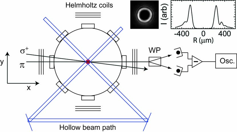
Figure 1: (Color online) Layout of experiment. Crossed hollow beams confine atoms to a 0.48mm diameter spot. Relay lenses for the hollow beams are not shown. Faraday pump and probe beams propagate along the x-axis to a balanced polarimeter. WP: Wollaston prism. Osc: Oscilloscope. Image of beam and cross sectional profile are shown.

Figure 1 shows the schematic layout of the experiment. The hollow beam is relayed to intersect itself by an $8f$ imaging relay, as described in Ref. Fatemi et al. (2007). Helmholtz coils on all three axes control the magnetic field. The hollow beams for our trap are formed by modifying the wavefront phase of a Gaussian beam with a reflective spatial light modulator (SLM). SLMs have found increasing value in cold atom manipulation experiments because of their ability to control trap parameters in a programmable manner and to produce traps with nontrivial intensity profiles Olson et al. (2007); Fatemi et al. (2007); McGloin et al. (2003); Pasienski and DeMarco (2008); Chattrapiban et al. (2006). The applied phase for the hollow beams used here has a profile $\Psi(\rho,\phi)=n\phi+f\lambda/(\pi\rho^{2})$, where $\rho$ and $\phi$ are cylindrical coordinates and $n$ is an integer. The second term is a lens function of focal length $f\approx 200$mm to focus the beam of wavelength $\lambda$ onto the atom sample. For high charge number beams ($n\geq 4$), we usually operate the trap a few centimeters away from the focal plane, where aberrations are reduced and the peak intensity is maximum Fatemi and Bashkansky (2007).

The light for the hollow beam is derived from a tunable extended cavity diode laser. It is amplified to 400 mW by a tapered amplifier, 200 mW of which is coupled into polarization-maintaining fiber. Residual resonant light from amplified spontaneous emission is filtered out by a heated vapor cell. The fiber output is collimated to a 1/$e^{2}$ waist of 1.71 mm, and modified by the SLM (Boulder Nonlinear Systems), which has $\approx$ 90% diffraction efficiency. The SLM has been calibrated at the pixel level to correct for wavefront distortion intrinsic to the SLM. An image of the beam is shown in the inset to Fig. 1. Our choice of $n=8$ is driven by the practical considerations of field-free confinement and large trap size, but these trap parameters can be adjusted with the SLM.

Our experiment begins with cold ⁸⁵Rb atoms derived from a magneto-optical trap (MOT). We confine $\approx 10^{7}$ atoms in a $\approx 500\mu$m diameter (1/$e^{2}$) cloud. The atoms are further cooled in a 10 ms long molasses stage to $\approx 10\mu$K, after which all MOT-related beams are extinguished. The hollow beam trap is on throughout the MOT loading, but can be switched off by an acoustooptic modulator. The Faraday spectroscopy is performed by similar technique as in Ref. Isayama et al. (1999). To perform these measurements, a pair of laser beams is used along the $x$-axis (Fig. 1). The atoms are optically pumped into the $F=3,m_{F}=3$ stretched state by a 20 $\mu$s $\sigma^{+}$ pulse connecting $F=3\rightarrow F^{\prime}=3$. This beam has 1/$e^{2}$ waist of 6.0 mm and has a peak intensity of $\approx 3I_{sat}$, where $I_{sat}$ is 1.6 mW/cm². This beam is retroreflected to prevent unidirectional momentum kicks, and a small amount of repumper light ($\approx 0.04I_{sat}$) is added during this pulse to keep the atoms in the $F=3$ hyperfine ground state. When this light is extinguished, the atoms begin precessing freely at the Larmor precession frequency $\omega_{L}=g_{F}\mu_{B}B/\hbar$, where $g_{F}$ is the gyromagnetic ratio, $\mu_{B}$ is the Bohr magneton, and $B$ is the magnetic field. For ⁸⁵Rb, $g_{F}\mu_{B}/\hbar=466.7415$ kHz/Gauss Alexandrov et al. (2004). A linearly polarized probe beam at a detuning $\Delta_{p}=2\pi\times 2.5$ GHz with $\simeq$20mW and 1/$e^{2}$ waist $\omega_{p}$ = 6.0mm passes through the atom cloud to a simple polarimeter consisting of a Wollaston prism that splits the probe beam into two orthogonal polarization states that are detected by a balanced photodetector. For these parameters, the photon scattering time from the probe beam is calculated to be $\tau_{p}\approx$2ms. The MOT region is imaged onto a pinhole along the axis of the probe beam so that only the portion of the probe that interacts with the confined atoms reaches the detector.

The hollow beam trap prevents the atoms from falling away from the interaction region during the probing process. The beam has 150 mW total power at the trap. We use a detuning $\Delta_{t}\approx 25$GHz (=0.05 nm) above the $F=3\rightarrow F^{\prime}=4$ transition. At the MOT, the hollow beam has a diameter of 0.48 mm, measured between maxima, and the peak intensity is $8.2\times 10^{4}$ mW/cm² for a trap depth $U\approx 2\hbar\Gamma\approx 3000E_{r}$, where $E_{r}$ is the recoil energy for ⁸⁵Rb. The gravitational potential energy across this trap is $\hbar\Gamma/6$. For these parameters, the peak scattering rate from the trapping beams would be $\gamma_{t}=1/\tau_{t}\approx 2\pi\times 3$kHz, but is reduced from this value by being trapped in the dark. Although we do not measure this value, we establish an upper bound to be $\gamma_{t}{\leq}2\pi\times 200$Hz.

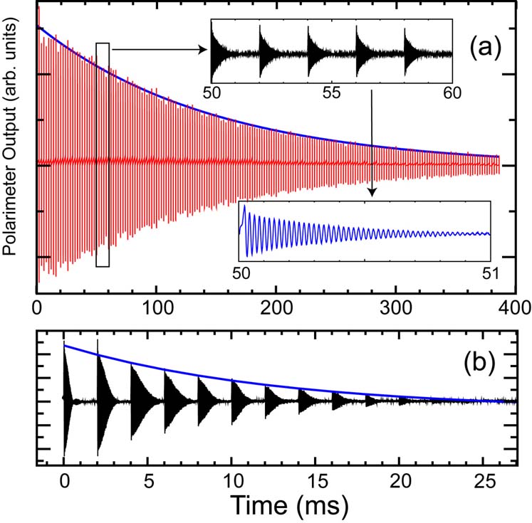
Figure 2: (Color online) Faraday signals for a) trapped sample; and b) untrapped sample. The untrapped atoms fall away from the probe region within 20 ms, while the trapped atoms remain with 150 ms time constant. Insets to (a) are expanded views of the raw data.

Each optical pumping event initiates the Larmor precession. Figure 2a shows 64 averages of 200 optical pumping cycles spaced 2 ms apart in the presence of the hollow beam trap and a bias magnetic field of $\approx 100$ mG along the $z$-axis. A single Larmor precession signal is shown in the lower inset to Fig. 2a. The envelope over all Larmor precession signals decays with a 1/$e$ time constant of $\approx 150$ ms. This decay is due primarily to the steady heating that occurs during each optical pumping cycle, which gradually boils atoms out of the trap. In contrast, Fig. 2b shows the signals without the hollow beam trap present. In this case, the atoms fall completely out of the probe beam detection window within 25 ms, with a 1/$e$ decay time of 13 ms, similar to that reported in Ref. Isayama et al. (1999). The signals in Fig. 2 are recorded immediately following the molasses phase of the MOT loading cycle. Over the first few pumping cycles, the envelope of the individual precession signals in Fig. 2b changes dramatically due to residual eddy currents in the vacuum chamber. Holding the atoms in an optical trap allows measurements to be performed after eddy currents have subsided, while also substantially increasing both the measurement window and the overall duty cycle.

For our parameters, each independent Larmor precession signal dephases with a submillisecond 1/$e$ decay time. This dephasing occurs from several factors, including spatial gradients and photon scattering from the trap and probe beams. Nonlinear Hamiltonian terms can also shorten the decay time of the signal, as described in Ref. Smith et al. (2004). These nonlinear terms depend on the angle between the polarization of the probe laser and the magnetic field. When the relative angle is $\approx$ 54^∘, the effects of these terms are eliminated. For this work, we operated at this relative orientation so that the dephasing occurs primarily through photon scattering. From Fig. 2, we find that the untrapped signals decay with a 1/$e$ time of $\approx$0.7ms. For the samples trapped in the hollow beam, we observe a slight reduction in the decay time to $\approx$0.5 ms. Thus we have an upper bound for $\gamma_{t}\leq 2\pi\times 200$Hz.

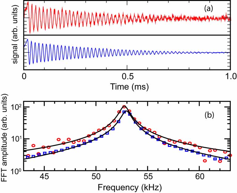
Figure 3: (Color online) a) Polarimeter output for single-shot data (top) and averaged data (bottom). b) Fast-Fourier transform (FFT) of data in (a). Fits to a Lorentzian profile are shown as solid lines. Single-shot (circles) and averaged (squares) data are shown.

In a gradient-free, static magnetic field, the voltage output of the polarimeter is an exponentially-damped sinusoid, $V(t)=$ Aexp(-$t/\tau$)sin$(2\pi\nu_{L}t+\phi)$, where A is the initial amplitude, $\tau$ is the 1/$e$ decay time, $\omega_{L}=2\pi\times\nu_{L}$ is the Larmor frequency, and $\phi$ is a phase. To determine $\nu_{L}$, the averaged data in each 2 ms probing window (Fig. 3a) are Fourier transformed (Fig. 3b). We fit these transforms to a Lorentzian, the center of which is $\nu_{L}$.

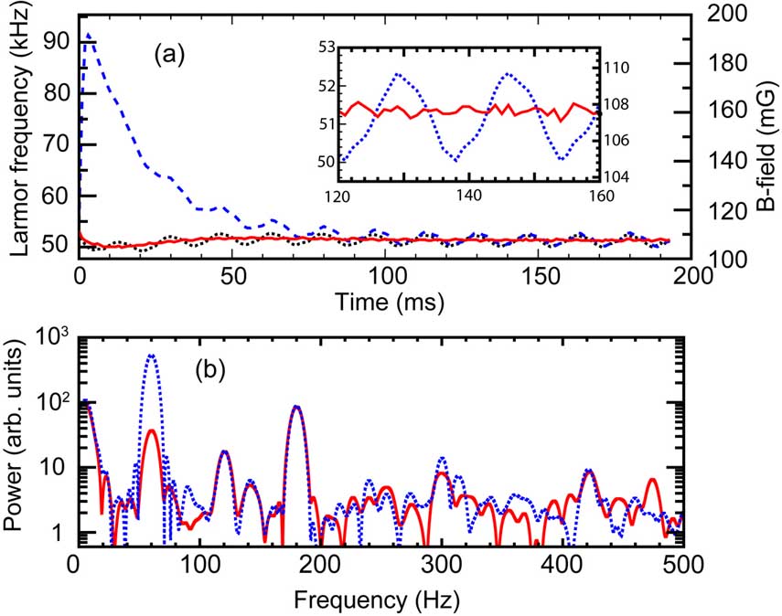
Figure 4: (Color online) a) Larmor precession frequency as a function of time with various levels of compensation. Dashed: no compensation; dotted: compensation of eddy currents, and solid: full compensation. Inset to (a) shows magnified view of compensation. Fluctuations in our Larmor precession are dominated by uncompensated harmonics of the AC line. b) Magnetic field spectrum with no compensation (dotted), and 60Hz compensation (solid).

In Fig. 4a, we plot $\nu_{L}(t)$ over 200 pumping cycles (64 averages) spaced 1 ms apart (dashed line). The signal displays two dominant sources of time-dependence. First, the exponential decay occurs from the metal vacuum chamber, which develops eddy currents when the MOT coils are extinguished. Due to the symmetry of our chamber, the eddy currents are along the axis of the MOT coils ($z$). The bias field of $\nu_{L}\approx 50$kHz for these measurements is also on the $z$-axis so that the eddy current field adds linearly to the bias field. The second source of time-dependent behavior is ambient AC magnetic fields in the room arising from power supply transformers, power strips, etc. We note that our experiment is triggered off the AC power line. We found that this field is also primarily along the $z$-axis, because the amplitude of the oscillation signal is independent of this bias field. An orthogonal component would add in quadrature and cause the amplitude to vary with the bias field. Additionally, an orthogonal, oscillating magnetic field component added in quadrature would show up at twice its oscillation frequency. Since the Larmor frequencies retrieved from Faraday spectroscopy determine the scalar magnetic field, full vector information is not acquired in a single shot, but can be acquired through multiple measurements Terraciano et al. (2007). Some information about magnetic field orientation can be obtained directly from the polarimeter signal (e.g. there is no spin precession if the $B$ field is parallel to the optical pumping axis), but that effect is outside the scope of this work.

For many applications, control over the magnetic field is required to sub-mG levels, especially those involving Raman transitions between magnetically sensitive states Boyer et al. (2004); Ringot et al. (2001); Terraciano et al. (2007); Kerman et al. (2000). As a simple application of the long measurement time capability, we demonstrate compensation of these time varying fields. We first compensate the effects of eddy currents, which produce an exponentially decaying magnetic field at the atom sample. This field decays with a 1/$e$ time of $\approx$20 ms (Fig. 4a). For a given MOT coil current setting, the eddy current amplitude is constant. We produce an opposing time-varying field flux by using a voltage-controlled current source (Kepco ATE15-15M). This current passes through a 20-turn Helmholtz pair of diameter 20 cm, width 2.5 cm, and separation 11.4 cm oriented along the MOT coil axis. The appropriate time variation is done by low-pass filtering of a step function whose amplitude is adjusted for optimum compensation. The result is shown in Fig. 4a (dotted line). Although this source of time variation is not canceled perfectly, the field beyond 25 ms is constant to within the 60 Hz field amplitude.

The ambient AC magnetic fields are primarily due to 60 Hz power line sources. By triggering our experiment from the power line, this source of magnetic field variation is reproducible and can be compensated. Without this triggering, the variations of a few mG observed in Fig. 4a would lead to significant shot-to-shot fluctuations of the field measurements. We produce an opposing field by adding a 60 Hz sinusoidally varying current to the bias coils. The current amplitude and phase are adjusted for optimum compensation. The result with all compensations applied is shown in the inset to Fig. 4a. The signal remains constant to within a standard deviation of 110 Hz (230 $\mu$G). Most of this residual field is due to higher AC line harmonics; in Fig. 4b, we show frequency spectrum of the magnetic field, which clearly shows higher harmonics at 180, 300, and 420 Hz. We suppressed the 60 Hz component by a factor of 20. With appropriate signal processing, the field measurements in our setup could be made in real time (with single-shot measurements as in Fig. 3) and be used as feedback control with a bandwidth determined by the Helmholtz compensation coils.

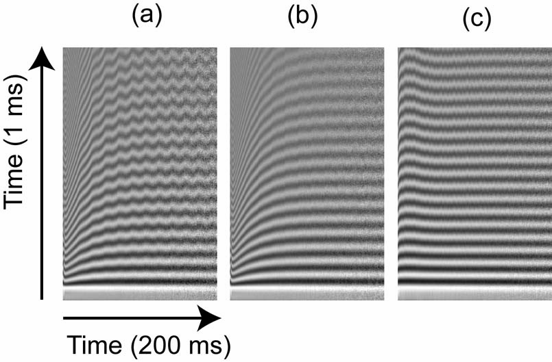
Figure 5: 2D image of data that exposes qualitative magnetic field features without FFT processing. (a) uncompensated, (b) 60 Hz compensation, c) full compensation.

Another way to visualize the time dependent signals, shown in Fig. 5a, is by converting the 1D data set of Fig. 2 to a 2D matrix. Each successive column contains the Larmor precession signal for subsequent triggers. This exposes time variations in an easily identifiable way with no FFT analysis. We show these images for the magnetic fields with no compensation, 60 Hz compensation and full compensation. A constant magnetic field shows up as a series of horizontal lines whose spacing is inversely proportional to $\omega_{L}$ (Fig. 5c).

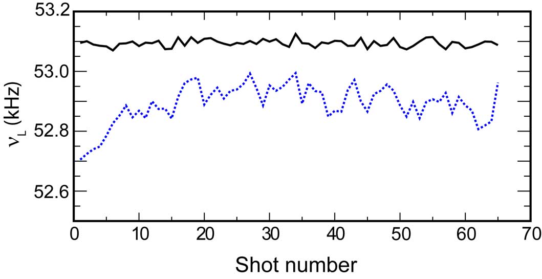
Figure 6: (Color online) Comparison of 64 data runs (dashed) to a simulated signal with white noise added to have similar SNR as the experiment (black). For clarity, the signals are offset from each other.

Because of the uncompensated field variations in our lab, our measurement uncertainty is dominated by systematic errors. To differentiate the systematic error from the random error, we measure the Larmor precession frequency in a 1 ms measurement window for 64 independent loading cycles at a trapping time of T = 100 ms. These scans are recorded at a 1 Hz rate. The result is shown in Fig. 6. There is a long term drift in our lab on the order of several seconds. Our time-domain signals have a signal-to-noise ratio (SNR) of $\approx$15 (Fig. 3a). For comparison, we simulated the expected Larmor signals for exponentially-damped sinusoids with the same SNR that had additive white noise (Fig. 6). For the experimentally measured case, we found a standard deviation, or single-shot error, in each 1 ms optical pumping cycle of $\delta\nu_{L}\approx$45Hz, or $\delta{B}\approx 100\mu$G (=10 nT), and for the simulated case, the error was $\delta\nu_{L}\approx$16 Hz, or $\delta{B}\approx 30\mu$G (=3 nT). This discrepancy is likely due to other sources, such as unwanted variations in the MOT coil current.

Our hollow beam traps are initially loaded with $N\approx 10^{6}$ atoms. The shot-noise-limited magnetic field measurement error due to atom number is $\delta{B}\simeq\left(\hbar/g\mu_{B}\right)(1/\sqrt{N\tau{T_{m}}})$, where $\tau$ is the spin-coherence time and $T_{m}$ is the measurement time Budker et al. (2002). Because we are measuring a rapidly varying field, $T_{m}=1\rm{-}2$ms, limiting $\delta{B}\approx 2\mu$G (=200 pT) in each optical pumping cycle. After T = 400 ms of trapping time, when there are only $\approx 10^{5}$ atoms remaining, this increases to $\approx 6\mu$G (=600 pT). Our measured values are above the shot noise limit due to the simple photodetection circuit we used and to incomplete optical pumping, which effectively reduces N.

For static magnetic fields, each measurement cycle through the total trap time can be averaged, effectively increasing $T_{m}$ to several hundred milliseconds and greatly increasing the shot-noise-limited sensitivity. Likewise, $\tau$ can be increased by using larger detunings for the probe and trapping beams. These blue-detuned traps are capable of capturing large enough atom numbers that measurements in the low pT range or better should be possible in a single MOT loading cycle over the entire measurement window.

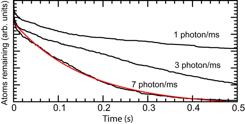
Figure 7: (Color online) Simulations of atom number remaining for different degrees of optical pumping. With no optical pumping or probe beams (longest-lived curve) the atoms still scattered $\approx$1 photon/ms from the trap beams. A curve fit is shown for the case of scattering 7 photons/ms. This time constant of 160 ms agrees well with our experimental value of 150 ms (Fig. 2).

For any trap depth, there is a trade-off between SNR and the number of possible field measurements allowed before the signal decays. SNR improves by increasing the number of atoms that are optically pumped or by decreasing the pump detuning Smith et al. (2003), but these approaches also boil the atoms out of the trap more quickly. For most of our results presented here, we only weakly pumped the atoms to reduce heating and to increase the number of optical pumping cycles we could achieve. In general, the dominant heating will occur from the $20\mu$s optical pumping phase of each cycle, during which several photons are scattered. As a rough estimate, the timescale for signal decay should be on the order of the time required for the average atom energy to equal the trap depth. This will occur after a time $T_{boil}=U/(\gamma_{tot}E_{r})$, where U is the trap depth, $\gamma_{tot}$ is the total scattering rate (including probe, trap, and optical pumping beams), and $E_{r}$ is the recoil energy. For our trap of $U~{}\approx 3000E_{r}$, and assuming $\approx 10$ scattered photons every 2ms optical pumping cycle, this gives $\approx 300$ pumping cycles before the atoms are boiled away.

To examine this boiling process more accurately, we perform Monte Carlo simulations of the atom dynamics within our trap for different total scattering rates. Within each time step, the atom’s momentum is changed with a probability determined by the local scattering rate for the probe and trap beams, as calculated by the Kramers-Heisenberg formula Miller et al. (1993). We performed these simulations for different optical pumping rates. In Fig. 7 we plot the number of atoms remaining as a function of time for varying degrees of scattering rates. For the case of 7 photons scattered every millisecond, we find an exponential decay of $\approx$160 ms, which is close to our observed value of $T_{boil}=150$ms. By turning off the probe and optical pumping beams in the simulation, we find that the trap beam scattering rate is $\gamma_{t}\approx 2\pi\times 100$Hz which agrees with our upper bound of $\gamma_{t}\leq 2\pi\times 200$Hz from the Faraday decay time.

Within our measurement error, we observed no effect of the trapping light on the Larmor frequency. Optically-induced Zeeman shifts that occur with elliptically polarized light Vengalattore et al. (2007); Romalis and Fortson (1999); Park et al. (2002) should be small, because the trap beam polarizations are linear and because of the low field confinement. Furthermore, any vector light shifts from the trap beams, confined to the $x-y$ plane, would add in quadrature to our applied magnetic field along $z$, reducing the effect on $\omega_{L}$ Romalis and Fortson (1999). We are currently studying the effects of trap geometry on the Larmor precession signals.

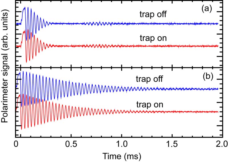
Figure 8: (Color online) Larmor precession signals with and without the trap light at two different relative orientations of the laser polarization with respect to the magnetic field. These were done at a) 0 degrees (revivals maximized) and b) 54 degrees (revivals suppressed).

The dominant source of nonlinear effects due to the laser fields is the probe light. As discussed in Ref. Smith et al. (2004), the tensor component to the light shift adds a nonlinear term to the spin Hamiltonian, whose magnitude is dependent on the angle between the laser polarization and the magnetic field. This Hamiltonian plays an important role in studies of quantum chaos and is useful for both nondestructive quantum state preparation and measurement Smith et al. (2004). For sufficiently large magnetic fields, the nonlinearity vanishes when the relative angle is $\theta$=arctan$(\sqrt{2})\approx 54^{\circ}$, but is maximized for $\theta=0$. We have verified that these nonlinear spin dynamics, which manifest themselves as revivals of the Faraday oscillation signal, can still be observed in these hollow beam traps. In Fig. 8, we show the Larmor precession signals for $\theta=0$ and $\theta=54^{\circ}$ both with the trap on continuously and with the trap switched off immediately prior to the optical pumping pulse. Thus the high duty cycle of the technique presented here may be of use for rapidly testing quantum state preparation procedures employing this nonlinearity.

We have demonstrated Faraday spectroscopy with high repetition rate, long measurement time, and submillimeter spatial resolution in a dark hollow beam optical trap. We used high-charge-number hollow laser beams to provide box-like confinement with near resonant light and low laser power. These traps can be sufficiently deep that several hundred Faraday measurements are possible before atoms are heated over the confining potential. We demonstrated a continuous magnetic field measurement over a period of 400 ms which enabled us to measure and compensate for time-varying magnetic fields. This work was funded by the Office of Naval Research and by the Defense Advanced Research Projects Agency.

References

- Budker et al. (2002) D. Budker, W. Gawlik, D. F. Kimball, S. M. Rochester, V. V. Yashchuk, and A. Weis, Rev. Mod. Phys. 74, 1153 (2002).
- Isayama et al. (1999) T. Isayama, Y. Takahashi, N. Tanaka, K. Toyoda, K. Ishikawa, and T. Yabuzaki, Phys. Rev. A 59, 4836 (1999).
- Labeyrie et al. (2001) G. Labeyrie, C. Miniatura, and R. Kaiser, Phys. Rev. A 64, 033402 (2001).
- Franke-Arnold et al. (2001) S. Franke-Arnold, M. Arndt, and A. Zeilinger, J. Phys. B 34, 2527 (2001).
- Smith et al. (2003) G. A. Smith, S. Chaudhury, and P. S. Jessen, J. Opt. B 5, 323 (2003).
- Geremia et al. (2005) J. M. Geremia, J. K. Stockton, and H. Mabuchi, Phys. Rev. Lett. 94, 203002 (2005).
- Vengalattore et al. (2007) M. Vengalattore, J. M. Higbie, S. R. Leslie, J. Guzman, L. E. Sadler, and D. M. Stamper-Kurn, Phys. Rev. Lett. 98, 200801 (2007).
- Chatraphorn et al. (2000) S. Chatraphorn, E. F. Fleet, F. C. Wellstood, L. A. Knauss, and T. M. Eiles, Appl. Phys. Lett. 76, 2304 (2000).
- Wildermuth et al. (2006) S. Wildermuth, S. Hofferberth, I. Lesanovsky, S. Groth, P. Krüger, J. Schmiedmayer, and I. Bar-Joseph, Appl. Phys. Lett. 88, 264103 (2006).
- Wang et al. (2005) Y.-J. Wang, D. Z. Anderson, V. M. Bright, E. A. Cornell, Q. Diot, T. Kishimoto, M. Prentiss, R. A. Saravanan, S. R. Segal, and S. Wu, Phys. Rev. Lett. 94, 090405 (2005).
- Romalis and Fortson (1999) M. V. Romalis and E. N. Fortson, Phys. Rev. A 59, 4547 (1999).
- Smith et al. (2004) G. A. Smith, S. Chaudhury, A. Silberfarb, I. H. Deutsch, and P. S. Jessen, Phys. Rev. Lett. 93, 163602 (2004).
- Chaudhury et al. (2007) S. Chaudhury, S. Merkel, T. Herr, A. Silberfarb, I. H. Deutsch, and P. S. Jessen, Phys. Rev. Lett. 99, 163002 (2007).
- Ozeri et al. (1999) R. Ozeri, L. Khaykovich, and N. Davidson, Phys. Rev. A 59, R1750 (1999).
- Friedman et al. (2002) N. Friedman, A. Kaplan, and N. Davidson, Adv. Atom. Mol. Opt. Phys. 48, 99 (2002).
- Kaplan et al. (2005) A. Kaplan, M. F. Andersen, T. Grunzweig, and N. Davidson, J. Opt. B 7, R103 (2005).
- Kulin et al. (2001) S. Kulin, S. Aubin, S. Christe, B. Peker, S. L. Rolston, and L. A. Orozco, J. Opt. B 3, 353 (2001).
- Fatemi and Bashkansky (2007) F. K. Fatemi and M. Bashkansky, Appl. Opt. 46, 7573 (2007).
- Fatemi et al. (2007) F. K. Fatemi, M. Bashkansky, and Z. Dutton, Opt. Express 15, 3589 (2007).
- Olson et al. (2007) S. E. Olson, M. L. Terraciano, M. Bashkansky, and F. K. Fatemi, Phys. Rev. A 76, 061404(R) (2007).
- McGloin et al. (2003) D. McGloin, G. Spalding, H. Melville, W. Sibbett, and K. Dholakia, Opt. Express 11, 158 (2003).
- Pasienski and DeMarco (2008) M. Pasienski and B. DeMarco, Opt. Express 16, 2176 (2008).
- Chattrapiban et al. (2006) N. Chattrapiban, E. A. Rogers, I. V. Arakelyan, R. Roy, and W. T. Hill, J. Opt. Soc. Am. B 23, 94 (2006).
- Alexandrov et al. (2004) E. B. Alexandrov, M. V. Balabas, A. K. Vershovski, and A. S. Pazgalev, Tech. Phys. 49, 779 (2004).
- Boyer et al. (2004) V. Boyer, L. J. Lising, S. L. Rolston, and W. D. Phillips, Phys. Rev. A 70, 043405 (2004).
- Ringot et al. (2001) J. Ringot, P. Szriftgiser, and J. C. Garreau, Phys. Rev. A 65, 013403 (2001).
- Terraciano et al. (2007) M. L. Terraciano, S. E. Olson, M. Bashkansky, Z. Dutton, and F. K. Fatemi, Phys. Rev. A 76, 053421 (2007).
- Kerman et al. (2000) A. J. Kerman, V. Vuletić, C. Chin, and S. Chu, Phys. Rev. Lett. 84, 439 (2000).
- Miller et al. (1993) J. D. Miller, R. A. Cline, and D. J. Heinzen, Phys. Rev. A 47, R4567 (1993).
- Park et al. (2002) C. Y. Park, J. Y. Kim, J. M. Song, and D. Cho, Phys. Rev. A 65, 033410 (2002).