The Structure of Narrative: the Case of Film Scripts

Abstract

We analyze the style and structure of story narrative using the case of film scripts. The practical importance of this is noted, especially the need to have support tools for television movie writing. We use the Casablanca film script, and scripts from six episodes of CSI (Crime Scene Investigation). For analysis of style and structure, we quantify various central perspectives discussed in McKee’s book, Story: Substance, Structure, Style, and the Principles of Screenwriting. Film scripts offer a useful point of departure for exploration of the analysis of more general narratives. Our methodology, using Correspondence Analysis, and hierarchical clustering, is innovative in a range of areas that we discuss. In particular this work is groundbreaking in taking the qualitative analysis of McKee and grounding this analysis in a quantitative and algorithmic framework.

Kewwords: data mining, data analysis, factor analysis, correspondence analysis, semantic space, Euclidean display, hierarchical clustering, narrative, story, film script

1 Introduction

As a framework for analysis of narrative in many areas of application, film scripts have a great deal to offer. We present quite a number of innovations in this work: quantifying and automating a range of qualitative ways of addressing pattern recognition in narrative; use of metric embedding using Correspondence Analysis, and ultrametric embedding through hierarchical clustering of a data sequence, in order to capture semantics in the data; and verifying experimentally the well foundedness of much that McKee [15] describes in qualitative terms.

Other than the data mining, two distinct levels of user are at issue here. Firstly and foremostly, we have the scriptwriter or screenwriter in mind. See [15] for a content-based description of the scriptwriting process. Secondly and more indirectly we have the movie viewer in mind. The feasibility of using statistical learning methods in order to map a characterization of film scripts (essentially using 22 characteristics) onto box office profitability was pursued by [7]. The importance of such machine learning of what constitutes a good quality and/or potentially profitable film script has been the basis for (successful) commercial initiatives, as described by [8]. The business side of the movie business is elaborated on in some depth in terms of avenues to be explored in the future, in [6].

A film script is semi-structured in that it is subdivided into scenes and sometimes other structural units. Furthermore there is metadata provided related to location (internal, external; particular or general location name); characters; day, night. There is also dialog and description of action in free text.

There are literally thousands of film scripts, for all genres, available and openly accessible (e.g. IMSDb, The Internet Movie Script Database, www.imsdb.com). While offering just one data modality, viz. text, there is close linkage to other modalities, visual, speech and often music.

An area of application of our work that is of particular importance is to movies for television. In contrast to a cinema movie, in television a serial dramatization is formulaic in its set of characters, their actions, location, and in content generally. In form it is even more formulaic, in length, initial scenes, positioning of advertisement breakpoints, and in other aspects of format. While screenwriting and subsequent aspects of cinema movie creation and development have been much studied (e.g. [15]), film writing for television has been less so. The latter is often team-based, and much more “managed” on account of its linkages with other dramatizations in the same series, or in closely related series. These properties of television serial dramatization lead, perhaps even more than for cinema movie, to a need for tools to quantitatively support script writing.

Film scripts constitute an outstanding template or model for other domains. One longer term goal of our work is for our tools to provide a platform for introducing interactivity into a movie. Interactivity with a film or video includes the following possible uses: (i) it provides an approach to developing interactive games; (ii) it allows for use in interactive and even immersive training and learning environments; and (iii) support is also feasible for use in the entertainment area, e.g. interactive television. Leveraging the existing corpus and “fanbase” of hit scripts to create new interactive versions could create a whole new sector of movie script based interactive games or filmed variant-sequels to famous movies that take the familiar in a different direction. The convergence of story-telling and narrative, on the one hand, and games, on the other, is explored in [9]. There and in [20], story graphs and narrative trees are used as a way to open up to the user the range of branching possibilities available in the story. A further longer term goal lies in the area of business analysis, especially in distributed, video-conferencing and other, settings. The narrative structure, similar to a film script, gives the analyst the framework for generating stories. Such narrative structures can be used for analysis of meetings, projects, dialogs, and any interactive sessions in real or virtual meetings.

Our work is hugely topical. A television serial episode costs between $2 to $3 million for one hour of television. New series are scripted and run on television channels and only then is viewer reaction used to determine their viability. This points to major potential savings. Understanding and supporting scriptwriting is crucial. An additional motivation is that the entertainment and cultural market is moving towards greater interactivity, and our work is of great potential here too.

The structure of the paper is as follows. In section 2, we provide essential background on the analysis approach taken. In section 3, we discuss the plausibility of taking text as a proxy for, or a practical and useful expression of, underlying content that we refer to as the story. In section 4, we describe briefly the data analysis algorithms that we use, providing citations to more detailed background reading.

In section 5 we study a number of aspects of the Casablanca movie script. In section 6, we turn attention to the television series, CSI (Crime Scene Investigation, Las Vegas).

Among important aspects of this work are the following. Firstly, we recast a number of issues discussed by McKee [15] in a quantitative and algorithmic form. Secondly, we employ Correspondence Analysis as a versatile data analysis framework. Since in Correspondence Analysis, each scene is expressed as an average of attributes used to characterize the scenes, and since each attribute is expressed as an average of the scenes they characterize, we have in Correspondence Analysis a way to represent and study semantics. Thirdly, our clustering of film script units (e.g., scenes) is innovative in a few ways, including respecting the sequence of film script units, and taking as input the “direction” of the film script content rather than having a more static framework for the input (which we found empirically to work less well in that it was far less discriminatory). This type of clustering captures the semantics of change. If scenes are very dissimilar they will be agglomerated late in the sequence of agglomerations.

2 Analysis of Change in Content Over Time

Analysis of a film script has everything to do with change in the course of the story, as we will now discuss, following McKee [15]. “The finest writing … arcs or changes … over the course of the telling” (p. 104, [15]).

A typical film has 40 to 60 “story events” or scenes. A scene is a story in miniature and must have activity or change. A scene will typically (with, of necessity, large variability) translate into 2 to 3 minutes of film. In our work we have examples of very short (one or two sentence) dialog or action descriptions in scenes. Compared to longer scenes, such short scenes can be equally revealing and significant. Units of action or behavior within a scene are termed beats by McKee. We will examine beats below in a case study using the Casablanca script. Ideally every scene is a turning point, in character behavior, or in changing the “values” involved from positive to negative or vice versa.

Moving upwards now in scale of units of film script, a sequence is a series of typically 2 to 5 scenes. A sequence expresses significant albeit moderate change. An act is a set of sequences expressing major impact. Acts are the “macro-structure of story” (p. 217, [15]). It is possible to have a one-act play or story, although this would be quite unusual.

The overall set of scenes (or sequences, or acts) is termed the plot. A climax in a sequence or act or plot is essential. It is final and irreversible (pp. 41–42, [15]). It is possible to distinguish between an open and a closed ending, respectively bringing finality versus leaving some issues hanging, and this does not alter the all-important climax. A sequence climax is of moderate importance, an act climax is of greater importance, and the plot climax is crucial. In this scheme of things, each scene is a turning point of limited, moderate or great importance in the context of the overall plot or story.

The degree of change is the difference between a scene and the scene that climaxes a sequence, or the scene that climaxes an act, or the overall and global climax of the plot. In the plot, there is no room for a missing scene, or a superfluous scene, or a misordering of scenes.

Rhythm and tempo are related to scene length. The former, rhythm, should be very variable in order to keep the viewer’s (reader’s) attention, allowing for a soft upper limit on the time-span of attention. Tempo can exemplify climax in two ways: firstly, through increasingly shortened scenes (or other units) leading up to a climax; and, secondly, through the climax being of clearly greater length than the preceding scene (in order to allow for sufficient time to elaborate and offload its content). A decrease in tempo, through a sudden increase in scene length, can be indicative of dénouement and climax. Increasing tempo, manifested through successively decreasing scene length, expresses a build-up of tension.

Our discussion up to now has been about story. We turn to types of structure. McKee [15] categorizes design into classical; minimalist or miniplot; and anti-structure or antiplot. In this categorization scheme for film, the minimalist design dovetails very well with television film and drama, with e.g. open ending, unreconciled internal conflict, and passive and/or multiple protagonists. Below we will explore case studies based on episodes of CSI (Crime Scene Investigation).

3 Justification for Textual Analysis of Film Script

In this section we address the issue of plausibility of appreciable analysis of content based on what are ultimately the statistical frequencies of co-occurrence of words.

Words are a means or a medium for getting at the substance and energy of a story (p. 179, [15]). Ultimately sets of phrases express such underlying issues (the “subtext”, as expressed by McKee, a term we avoid due to possible confusion with subsets of text) as conflict or emotional connotation (p. 258). We have already noted that change and evolution is inherent to a plot. Human emotion is based on particular transitions. So this establishes well the possibility that words and phrases are not taken literally but instead can appropriately capture and represent such transition. Text, says McKee, is the “sensory surface” of a work of art (counterposing it to the subtext, or underlying emotion or perception).

Simple words can express complex underlying reality. Aristotle, for example, used words in common usage to express technically loaded concepts ([18], p. 169), and Freud did also.

Best practice in film script writing includes the following. Present tense dominates all ([15], p. 395): “The ontology of the screen is an absolute present tense in constant vivid movement” (emphasis in original). Clipped diction is needed. Generic nouns are avoided in favor of specific terms, and similarly adjectives and adverbs are to be avoided. The verb “to be” is to be avoided because: “Onscreen nothing is in a state of being; story life is an unending flux of change, of becoming” (p. 396). Simile and metaphor are out, as is any explicit positioning of context on behalf of the reader of the script or viewer of the film.

4 Methodology: Euclidean Embedding through Correspondence Analysis, and Clustering the Succession of Film Script Scenes

We have already noted (section 1) some novel aspects of our methodology. We begin with the display of data (e.g., scenes and/or words) where visualization of relationships is greatly facilitated by having a Euclidean embedding. We show how Correspondence Analysis furnishes such a metric space embedding of the information present in the film script text, and furthermore how this facilitates an ultrametric (i.e. hierarchical) embedding that takes account of the temporal, semantic dynamic of the film script narrative.

4.1 A Note on Correspondence Analysis

Correspondence Analysis [18] takes input data in the form of frequencies of occurrence, or counts, and other forms of data, and produces such a Euclidean embedding. The Appendix provides a short introduction to Correspondence Analysis and hierarchical clustering.

We start with a cross-tabulation of a set of observations and a set of attributes. This starting point is an array of counts of presence versus absence, or frequency of occurrence. From this input data, we can embed the observations and attributes in a Euclidean space. This factor space is mathematically optimal in a certain sense (using the least squares criterion, which is also Huyghens’ principle of decomposition of inertia). Furthermore a Euclidean space allows for easy visualization that would be more awkward to arrange otherwise.

A third reason for the particular embedding used for the observations and attributes in the Euclidean factor space is that weighting of observations and attributes is handled naturally in this framework. The issue of weighting has to be addressed somehow, with one option being to treat the set (of observations or of attributes) as identically weighted, and hence of equal a priori importance. Very often either observations or attributes follow a power law: examples of such power laws include Zipf’s law (in natural language texts, the word frequency is inversely proportional to its rank), the Pareto distribution in economics, and many others [19]. Correspondence Analysis handles weighting of observations and attributes at the “core” of its algorithm [18].

Application of the power law property to social networks has included the network of movie actors [19]. As counterposed to such work, our interest is in analyzing a time series of data. The succession of scenes in a movie, or acts in a play, exemplify this.

4.2 Input Data Used

We take all words into account in the semi-structured texts that are provided by film (or television program) scripts. Punctuation is ignored. Upper case is converted to lower case for our purposes. Words must be at least two characters in length. Any numerical figure, or term beginning with a numerical, is ignored. We have already noted above (section 3; see also the case studies and discussion in [18]) why the use of all words in this way is, in principle, feasible and justified.

Occurrences or presence/absence data therefore are the point of departure. Each scene is cross-tabulated by the set of all words so that, in this cross-tabulation table, at the intersection of scene $i$ and word $j$ we have a presence (1) or absence (0) value. To employ notions of change or proximity between scenes, we need this data to be appropriately represented in a numerically well-defined semantic space. This is provided by mapping the frequencies of occurrence data into a Euclidean space, using Correspondence Analysis.

4.3 Hierarchical Agglomerative Clustering Respecting Sequence

Unusually in this work, we use hierarchical clustering taking a sequence of film script units (e.g., scenes) into account. Our motivation is the following: large ultrametric or tree distances derived from the hierarchy have a ready interpretation in terms of change. A brief introduction is provided in the Appendix. A short discussion follows.

Hierarchical clustering is carried out through a sequence of agglomerations of successive scenes or of clusters (or temporal segments or intervals) of successive scenes. Respect for the sequentiality of the scenes is ensured through the requirement that agglomerands must be adjacent. In addition to this, the least dissimilar scenes are checked, with the criterion being: merge two clusters when the greatest dissimilarity between cluster members (scenes) is minimal. The least dissimilar pair of scenes, considering two potential agglomerands, is what we use as our agglomeration criterion. This is the contiguity-constrained complete link hierarchical clustering method. Apart from heuristic reasons for favoring it, it has some further properties that will now be discussed briefly.

The sequence-related adjacency requirement must take into consideration whether an agglomerative clustering method would give rise to an inversion, i.e., a later agglomeration in the sequence of agglomerations would have an associated criterion value that is less than the previous criterion value. It is not hard to appreciate that our desire to have gradations of distance represented by the dendrogram would be negated, and severely so, by such absence of the monotonicity of criterion value, which amounts to a contradiction in interpretation of the dendrogram.

It is shown in [17] that two algorithms are feasible. What is involved here is sketched out as follows.

Continuity-constrained single link hierarchical clustering is simultaneously hierarchical clustering on the spanning graph. This is easy to implement (inefficiently): just fix an infinite (or very large) distance between non-contiguous pairs and proceed to use single link hierarchical clustering [17].

The complete link method, with the constraint that at least one member of each of the two clusters to be agglomerated be contiguous, is guaranteed not to give rise to inversions. The $O(n^{2})$ time, $O(n^{2})$ space algorithm for the complete link method, based on the nearest neighbor chain (see [17]), is easily modified to include an additional testing of contiguity whenever a linkage in the nearest neighbor chain is created.

In this work we use the latter, in view of the well-balanced hierarchies typically produced, [16].

5 Casablanca Film Script Analysis

5.1 Data Used

Based on the unpublished 1940 screenplay by Murray Burnett and Joan Allison, [3], the Casablanca script by Julius J. Epstein, Philip G. Epstein and Howard Koch led to the film directed by Michael Curtiz, produced by Hal B. Wallis and Jack L. Warner, and shot by Warner Bros. between May and August 1942. We used the script from The Internet Movie Script Database, IMSDb (www.imsdb.com).

The Casablanca film script comprises 77 successive scenes. All told, there were 6710 words in these successive scenes.

The source text for the 77 scenes, including metadata, varied between just 5 words, and 1017 words (scene 22). Typical Zipf distributional behavior is seen in the marginals. All words were used, following the imposing of lower case throughout. This was subject only to words being longer than one character. No stemming or other preprocessing was used. The top word frequencies were interesting: the, 965; rick, 689; you, 651; to, 574; and, 435; in, 332; of, 319; renault, 284; it, 271; ilsa, 256; laszlo, 255; he, 236; is, 232; at, 192; that, 171; for, 158; we, 151; on, 149; strasser, 135. The numerically high presence of personal names is quite unusual relative to more general texts, and characterizes this film script text. A major reason for this is that character names head up each dialog block.

Casablanca is based on a range of miniplots. This occasions considerable variety. Miniplots include: love story, political drama, action sequences, urbane drama, and aspects of a musical. The composition of Casablanca is said by McKee [15] to be “virtually perfect” (p. 287).

5.2 Analysis of Casablanca’s “Mid-Act Climax”, Scene 43

To illustrate our methodology, applied below to scenes, we look first in depth at one particular scene.

This scene is discussed in detail in McKee [15], who subdivides it into 11 successive beats (here understood as subscenes). It relates to Ilsa and Rick seeking black market exit visas. Beat 1 is Rick finding Ilsa in the market. Beats 2, 3 and 4 are rejections of him by Ilsa. Beats 5 and 6 express rapprochement by both characters. Beat 7 is guilt-tripping by each in turn. Beat 8 is a jump in content: Ilsa says she will leave Casablanca soon. In beat 9, Rick calls her a coward, and Ilsa calls him a fool. Beat 10 is a major push by Rick, essentially propositioning her. In the climax in beat 11, all goes to rack and ruin as Ilsa says she was married to Laszlo all along, and Rick counters that she is a whore.

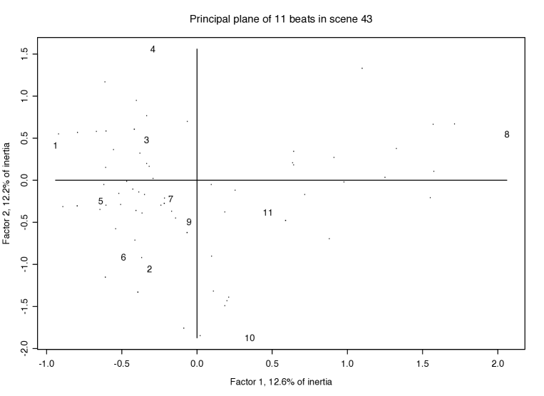
Figure 1: Correspondence Analysis of the scene 43, which crosses (with presence/absence values) 11 successive beats (numbers) with, in total, 210 words (dots: not labeled for clarity here).

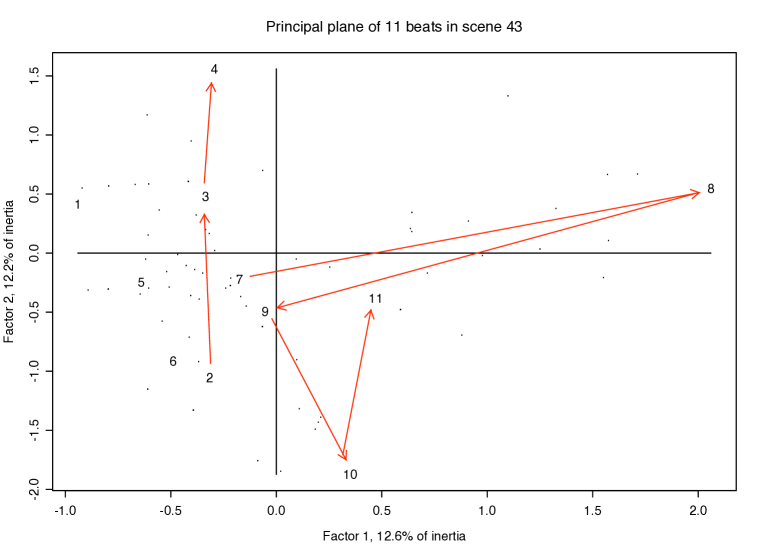
Figure 2: As Figure 1, with some major movements from beat to beat noted and discussed in the text.

Figure 1 shows the best planar projection of the beats. The dots show the locations of the words. The importance of the factors is defined by the percentages of inertia explained by the factors (see Appendix for background details). We could certainly look further at what words are closest to scene 8. (They are words having to do with Ilsa announcing that she will leave Casablanca.)

Look though at the following aspects of Figure 1, as illustrated in Figure 2. Beats 2, 3 and 4 are moving nicely in one direction, so we can claim that moving in the positive direction of the ordinate (vertical axis) is reinforcement of Ilsa’s rejection of Rick. As against this, movement in the negative direction of the ordinate expresses rapprochement by Ilsa and Rick: look at beat 10. Beat 8 is way off, and for Rick points to a real possibility of losing the game (of re-captivating Ilsa). The climax in beat 11 moves distinctly away from Rick’s aspirations as expressed in beat 10.

The length of the beat can show a lead-up to a climax in the scene, as noted in section 2. We see this very well in the beats of scene 43: the final five beats have lengths (in terms of presence of the words we use) of 50, 44, 38, 30, and then in the climax beat, 46. Earlier beats vary in length, with successive word counts of 51, 23, 99, 39, 30, 17.

The overall change in this scene, scene 43, is defined by the difference between closing and opening beats. Given the Correspondence Analysis output, where we have a Euclidean embedding taking care of weighting and normalization on both beat and word sets, we can easily take the full-dimensionality embedding (unlike the 2-dimensional projection seen in Figure 1) and determine this distance between beat number 1 and beat number 11. As suggested very strongly by Figure 1, this distance will not necessarily be the greatest distance among successive beats.

We reiterate that Figure 1 provides us with a planar projection of the beats, which is optimal in a least squares sense, but is of necessity an approximation to the full-dimensionality clouds of beat, and word, points. The quality of this best fit approximation is roughly 24.8% (i.e., the sum of inertias explained by the two axes of Figure 1) of the information content of the overall cloud, considered as either the cloud of beats, or the cloud of words.

For clustering the data displayed in Figure 1 we will use the full dimensionality. We have noted above some of the changes in direction in the succession of beats, as displayed in Figure 1: 2, 3 and 4 following a particular sweep; 10 reverses this; and so on. Let us therefore look at the clustering of beats based solely on changes in direction or orientation. In the full-dimensionality Correspondence Analysis embedding we will look not at the positions of the beats but instead at their correlation with the factors (i.e., axes or coordinates). Changes from one beat’s correlations with all factors, to those of the next beat, admirably express change in orientation of these successive beats.

Figure 3 shows the hierarchical clustering of the correlations (with all factors) for the 11 successive beats, using the sequence- or chronology-constrained agglomerative method discussed in section 4.3. Note how beats 2, 3, 4 are clustered together; how 5, 6, 7 have a certain unity too; and in particular how beat 8 is a sort of major caesura in the overall sequence of beats.

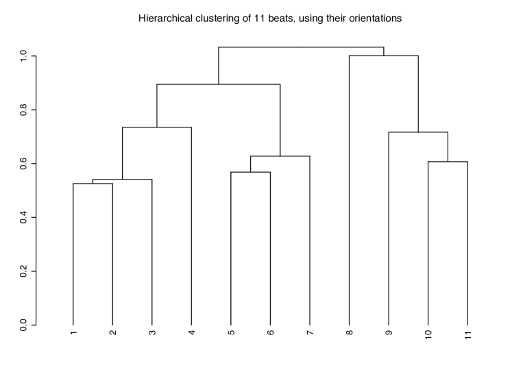
Figure 3: Hierarchy of the 11 beats in scene 43, using the relationships of beats defined from changes in orientation.

We do not find everything needed to understand the beat succession of scene 43 of Casablanca in the vantage points offered by Figures 1 and 3. But we are gathering very useful perspectives on this scene. To see how useful this is, let us carry out a benchmarking or baselining of what we see against an alternative of a randomized set of 11 beats in scene 43.

5.3 The Specific Style of a Film Script

Arising out of our exploration so far, we will use the following indicators of style and structure. To be usable across different film scripts, we must look at aggregate quantities. Here we will use first and second order moments. We continue to use scene 43 of Casablanca, with its 11 successive, constituent beats.

The attributes used are as follows.

1. Attributes 1 and 2: The relative movement, given by the mean squared distance from one beat to the next. We take the mean and the variance of these relative movements. Attributes 1 and 2 are based on the (full dimensionality) factor space embedding of the beats.

2. Attributes 3 and 4: the changes in direction, given by the squared difference in correlation from one beat to the next. We take the mean and variance of these changes in direction. Attributes 3 and 4 are based on the (full dimensionality) correlations with factors.

3. Attribute 5 is mean absolute tempo. Tempo is given by difference in beat length from one beat to the next. Attribute 6 is the mean of the ups and downs of tempo.

4. Attributes 7 and 8 are, respectively, the mean and variance of rhythm given by the sums of squared deviations from one beat length to the next.

5. Finally, attribute 9 is the mean of the rhythm taking up or down into account.

For the Casablanca scene 43, we found the following as particularly significant. We tested the given scene, with its 11 beats, against 999 uniformly randomized sequences of 11 beats. If we so wish, this provides a Monte Carlo significance test of a null hypothesis up to the 0.001 level.

• In repeated runs, each of 999 randomizations, we find scene 43 to be particularly significant (in 95% of cases) in terms of attribute 2: variability of movement from one beat to the next is smaller than randomized alternatives. This may be explained by the successive beats relating to coming together, or drawing apart, of Ilsa and Rick, as we have already noted.

• In 84% of cases, scene 43 has greater tempo (attribute 5) than randomized alternatives. This attribute is related to absolute tempo, so we do not consider whether decreasing or increasing.

• In 83% of cases, the mean rhythm (attribute 7) is higher than randomized alternatives.

5.4 Analysis of All 77 Scenes

The clustering hierarchy that we focus on here is based on the orientation of the scenes. This we do by taking any given scene’s correlations with the factors. We have observed earlier that the flow of the story, in relative terms, involves many “backs and forths” or “tos and fros”. This justifies our reason for looking at whether or not a group of scenes maintains an approximately similar orientation for some time, and how dramatic are the changes in direction.

Our clustering algorithm takes the sequence of scenes into account. As such, it offers a way to look at change over this sequence progression. We could well construct such a hierarchy of changes on data other than scene orientation or direction. We could use tempo or rhythm, for example. However, orientation or direction serves us very well and provides, already, useful insight into deep structure.

In Figure 4 we see how different scene 1 is, relating to narrated scene-setting of the Second World War. Scene 25 is a flashback to Paris in the spring. Scene 39 is set in a black market in Casablanca, where a Native and a Frenchman appear, but not any of the central characters. In this hierarchy we can see a pronounced redirection of the story in scenes 38, 39 and 40. (Note how the ultrametric distance between scene 39, on the one hand, and scene 38 or any preceding scene on the other hand, is relativley very great. The ultrametric distance between scene 39 and scene 40 is even greater.) In scene 38, Laszlo and Ilsa are in Renault’s office, clarifying their visa situation. The black market of scene 39 points the finger at Signor Ferrari, to be found at the Blue Parrot cafe. Scene 40 is then at the Blue Parrot. The essential issue of Laszlo’s role and problem of getting a visa is revealed in these scenes. In the overall story-line, these scenes are more or less right at the mid-point. The pairing off of scenes at the end (74 and 75, 76 and 77: respectively, airport, hangar, road, hangar) is very much in keeping with the content of these scenes. Together they represent the climax scenes.

A potential use of Figure 4 is to provide an indication of possible commercial breaks between acts or sequences of scenes, such that these breaks are derived automatically from the screenplay and without the writer explicitly marking them in the text. In cinema movie such breaks are not pre-planned. The hierarchy provides a visualization allowing comparison between the writer’s intentions and one (albeit insightful) view of where these breaks are found to be located, coupled with the strength of the breaks.

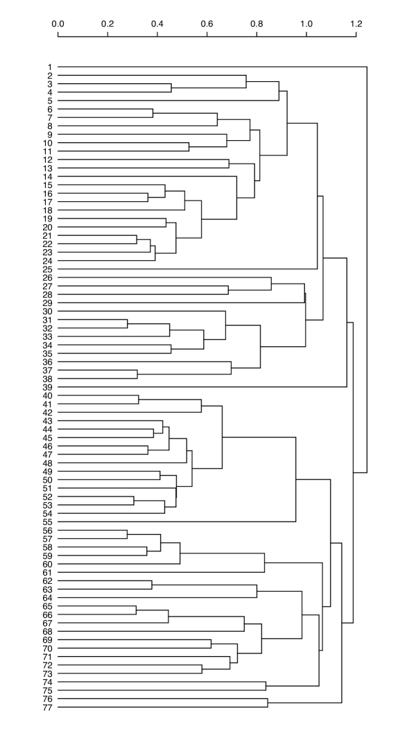
Figure 4: Hierarchy of the 77 scenes, respecting the sequence, based on the characterization of the 77 scenes by the set of all words used in the scenes. The directional information (i.e., correlations with the factors) associated with the scenes is used.

We again looked as style and structure, using 999 randomizations of the sequence of 77 scenes. Some interesting conclusions were garnered.

• As for the case of beats in scene 43, we find that the entire Casablanca plot is well-characterized by the variability of movement from one scene to the next (attribute 2). Variability of movement from one beat to the next is smaller than randomized alternatives in 82% of cases.

• Similarity of orientation from one scene to the next (attribute 3) is very tight, i.e. smaller than randomized alternatives. We found this to hold in 95% of cases. The variability of orientations (attribute 4) was also tighter, in 82% of cases.

• Attribute 6, the mean of ups and downs of tempos is also revealing. In 96% of cases, it was smaller in the real Casablanca, as opposed to the randomized alternatives. This points to the “balance” of up and down movement in pace.

6 Television Series Script Analysis

Our discussion so far has been for the Casablanca movie. Now we turn to television drama, for which other constraining aspects hold (such as length, and inter- as well as intra-cohesion and homogeneity).

We took three CSI (Crime Scene Investigation, Las Vegas – Grissom, Sara, Catherine et al.) television scripts from series 1:

• 1X01, Pilot, original air date on CBS Oct. 6, 2000. Written by Anthony E. Zuiker, directed by Danny Cannon.

• 1X02, Cool Change, original air date on CBS, Oct. 13, 2000. Written by Anthony E. Zuiker, directed by Michael Watkins.

• 1X03, Crate ’N Burial, original air date on CBS, Oct. 20, 2000. Written by Ann Donahue, directed by Danny Cannon.

Note the differences between writers and directors in most cases. This lends weight to our goal of furnishing the producer and director teams with a platform for automatically or semi-automatically assessing quality of product. We will refer to these scripts as CSI-101, CSI-102 and CSI-103. All film scripts were obtained from TWIZ TV (Free TV Scripts & Movie Screenplays Archives), http://twiztv.com

From series 3, we took another three scripts.

• 3X21, Forever, original air date on CBS, May 1, 2003. Written by Sara Goldfinger, directed by David Grossman.

• 3X22, Play With Fire, original air date on CBS, May 8, 2003. Written by Naren Shankar and Andrew Lipsitz, directed by Kenneth Fink.

• 3X23, Inside The Box, original air date on CBS, May 15, 2003. Written by Carol Mendelsohn and Anthony E. Zuiker, directed by Danny Cannon.

We will refer to these as CSI-321, CSI-322 and CSI-323.

An example of a very short scene, scene 25 from CSI-101, follows.

[INT. CSI - EVIDENCE ROOM -- NIGHT]

(WARRICK opens the evidence package and takes out the shoe.)

(He sits down and examines the shoe.  After several dissolves, WARRICK
opens the
lip of the shoe and looks inside.  He finds something.)

WARRICK BROWN:  Well, I’ll be damned.

(He tips the shoe over and a piece of toe nail falls out onto the table.  He
picks it up.)

WARRICK BROWN:  Tripped over a rattle, my ass.

We see here scene metadata, characters, dialog, and action information, all of which we use. Frontpiece, preliminary or preceding storyline information, and credits were ignored by us. We took the labeled scenes. The number of scenes in each movie, and the number of unique, 2-characters or more, words used in the movie, are listed in Table 1. All punctuation was ignored. All upper case was converted to lower case. Otherwise there was no pruning of stopwords. The top words and their frequencies of occurrence were:

the 443; to 239; grissom 195; you 176; and 166; gil 114; catherine 105; of 89; he 85; nick 80; in 79; on 79; it 78; at 76; ted 66; sara 65; warrick 65; …

Script	No. scenes	No. words
CSI-101	50	1679
CSI-102	37	1343
CSI-103	38	1413
CSI-321	39	1584
CSI-322	40	1579
CSI-323	49	1445

Table 1: Numbers of scenes in the plot, and numbers of unique (2-letter or more) words.

In order to equalize the Zipf distribution of words, and to homogenize the scenes and words by considering profiles (as opposed to raw data), as before we embedded the set of scenes in a Euclidean factor space in all cases, using Correspondence Analysis. We then clustered the full dimensionality factor space, using the hierarchical agglomerative algorithm that took into account the sequence of scenes, viz. the sequence-constrained complete link agglomerative method. To capture the “drift” of direction of the story, again like before, we used correlations rather than projections.

Figure 5: Sequence-constrained complete link hierarchy for CSI episode 101. Orientations (full dimensionality) were used for each of the 50 scenes.

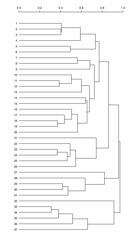
Figure 6: Sequence-constrained complete link hierarchy for CSI episode 102. Orientations (full dimensionality) were used for each of the 37 scenes.

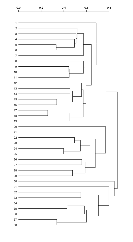
Figure 7: Sequence-constrained complete link hierarchy for CSI episode 103. Orientations (full dimensionality) were used for each of the 38 scenes.

Figures 5, 6 and 7 show the results obtained.

To focus discussion of internal structure which can be appreciated in these figures, let us look at where commercial breaks are flagged. While other considerations are important, like elapsed time from the start, it is clear that continuity of content is also highly relevant. Television episodes are written to create minor cliffhangers at the commercial breaks and therefore if the breaks can be identified by our datamining approach there is prima facie evidence for the finding of deep structures within screenplays. Four commercial breaks are flagged in the script of CSI-101, and three in the scripts of CSI-102 and CSI-103.

For CSI-101, Figure 5, these commercial breaks, as given in the script, were between scenes 4 and 5; 14 and 15 (substantial change noticeable in Figure 5); and 32 and 33. The change in direction in the climax scene, scene 50, is clear. The early scenes, 1 up to 6, are distinguishable from the scenes that follow.

For CSI-102, Figure 6, the commercial breaks were between scenes 4 and 5; 12 and 13; and 22 and 23. The climax here appears to be a collection of scenes, from 33 to 37.

Finally, for CSI-103, Figure 7, the commercial breaks were between scenes 1 and 2 (clear change); 9 and 10; and 29 and 30 (clear change).

We summarize these findings as follows. There is occasionally a very strong link between commercial breaks and change in thematic content as evidenced by the hierarchy. In other cases we find continuity of content bridging the gap of the commercial breaks.

Programs CSI-102 and CSI-103 are perhaps clearer than CSI-101 in having a more balanced subdivision. For CSI-102, we would put this subdivision as from scenes 1 to 20; 21 to 26; 27 to 31; and 32 to 37. For CSI-103, we would demarcate the plot into scenes 1 to 19; (20 or) 21 to 29; and 30 to 38.

As in section 5.3, we looked at the characteristics of style in the scripts. For a given script, we characterized it on the basis of our nine attributes. Then we randomized the order of the scenes comprising the script. So the plot (or story) was identical in terms of the scenes that constitute it. But the plot was lacking in sense – in style and in structure – to the extent that the scenes were now in a random order. Such a randomized plot was also characterized on the basis of our nine attributes. We carried out 999 such randomizations. When an attribute’s value for the real script was found to be less than or greater than 80% of the randomized plots, then we report it in Table 2. Our significance threshold of 80% was set at this value to be sufficiently decisive. It was rounded to an integer percentage in all cases.

program script	attribute	program $\leq/\geq$	% of cases
CSI-101	1	$\leq$	87%
CSI-101	3	$\leq$	93%
CSI-101	5	$\leq$	84&
CSI-101	6	$\geq$	84%
CSI-101	7	$\leq$	90%
CSI-101	9	$\leq$	88%
CSI-102	1	$\leq$	95%
CSI-102	2	$\leq$	95%
CSI-102	3	$\leq$	95%
CSI-102	5	$\geq$	81%
CSI-102	6	$\leq$	81%
CSI-103	2	$\leq$	88%
CSI-103	3	$\leq$	95%
CSI-103	4	$\geq$	83%
CSI-103	6	$\leq$	88%
CSI-103	9	$\leq$	88%
CSI-321	1	$\leq$	83%
CSI-321	2	$\geq$	91%
CSI-322	1	$\leq$	92%
CSI-322	3	$\leq$	97%
CSI-322	4	$\leq$	86%
CSI-322	6	$\geq$	86%
CSI-323	1	$\leq$	92%
CSI-323	8	$\leq$	81%
CSI-323	9	$\leq$	81%

Table 2: Shown are how and where the six television movies considered are unique in structure and style. For a particular attribute (see section 5.3 for description) the program script was different from randomized scene sequences in the indicated % of cases.

In regard to Table 2 we recall from section 5.3 that attributes 1 and 2 are first and second moments, respectively, of relative movement from one scene to the next. Attributes 3 and 4 are first and second moments of relative orientation from one scene to the next. Attributes 5 and 6 relate to tempo. Attributes 7, 8 and 9 relate to rhythm.

Furthermore whether our script is less than or greater than the randomized alternatives – cf. column 3 of Table 2 – can be understood as follows. If the “less than or equal to” case applies we can view this as our script being more compact or more parsimonious or more smooth or low frequency, for the particular attribute at issue, relative to the great bulk of randomized alternatives. Where the “greater than or equal to” case applies, then we can see something exceptional in the way that the plot is handled.

In Table 2, attribute 1 (mean relative movement) is a strong characterizing marker for all scripts, save one. This attribute is “compact” for the real script (in the sense in which we have used this term of “compact” in the last paragraph, with reference to column 3 of Table 2). Attribute 3 (mean relative reorientation) is a good characterizing marker for four of the six scripts. Attribute 9 (rhythm) is also a good marker for three of the six scripts.

Our Monte Carlo procedure is a rigorous one for assessing significance of patterns in the filmscript data. As we have demonstrated it allows us to validate unique semantic properties underlying the “sensory surface” (McKee) of the filmscripts.

7 Conclusions

The basis for accessing semantics in provided by (i) Correspondence Analysis, where each scene is an average of words or other attributes that characterize it, and each attribute is an average of scenes that are characterized; and (ii) in the hierarchical clustering of the sequence of scenes, relative change is modeled by the dendrogram structure.

We have made excellent progress in this work on having the qualitative precepts of McKee [15] both quantified and operationalized. Our assessments of the Casablanca movie, and the six CSI episodes, show that there is a great deal of commonality in style and structure between film and television.

We have taken into account both the linear and the hierarchical relationships in the plot, expressing the story. The units used were beats (i.e., subscenes) and scenes, essentially, with the hierarchical clusterings revealing larger scale structures (beginning scenes; climax scenes; and the halves, or thirds, or whatever segments were revealed as appropriate for the entire plot).

Let us look now at how our work is of importance for the study of style and structure in narrative, in general.

Chafe [4], in analyzing verbalized memory, used a 7-minute 16 mm color movie, with sound but no language, and collected narrative reminiscences of it from human subjects, 60 of whom were English-speaking and at least 20 spoke/wrote one of nine other languages. Chafe considered the following units.

1. Memory expressed by a story (memory takes the form of an “island”; it is “highly selective”; it is a “disjointed chunk”; but it is not a book, nor a chapter, nor a continuous record, nor a stream).

2. Episode, expressed by a paragraph.

3. Thought, expressed by a sentence.

4. A focus, expressed by a phrase (often these phrases are linguistic “clauses”). Foci are “in a sense, the basic units of memory in that they represent the amount of information to which a person can devote his central attention at any one time”.

The “flow of thought and the flow of language” are treated at once, the latter proxying the former, and analyzed in their linear and hierarchical structure by [4, 13, 14], among others. Filmscript affords us clear boundaries between the units of text that are analyzed. For more general text, we must consider segmentation. Examples of text segmentation to open up the analysis of style and structure include [12, 2, 11, 10, 5, 21].

We have shown in this work how useful the story expressed in a film or television movie script can be, in order to provide a framework for analysis of style and structure.

Appendix: Correspondence Analysis and Hierarchical Clustering

Analysis Chain

Correspondence Analysis, in conjunction with hierarchical clustering, provides what could be characterized as a data analysis platform providing access to the semantics of information expressed by the data. The way it does this is (i) by viewing each observation or row vector as the average of all attributes that are related to it; and by viewing each attribute or column vector as the average of all observations that are related to it; and (ii) by taking into account the clustering and dominance relationships given by the hierarchical clustering.

The analysis chain is as follows:

1. The starting point is a matrix that cross-tabulates the dependencies, e.g. frequencies of joint occurrence, of an observations crossed by attributes matrix.

2. By endowing the cross-tabulation matrix with the $\chi^{2}$ metric on both observation set (rows) and attribute set (columns), we can map observations and attributes into the same space, endowed with the Euclidean metric.

3. A hierarchical clustering is induced on the Euclidean space, the factor space.

4. Interpretation is through projections of observations, attributes or clusters onto factors. The factors are ordered by decreasing importance.

There are various aspects of Correspondence Analysis which follow on from this, such as Multiple Correspondence Analysis, different ways that one can encode input data, and mutual description of clusters in terms of factors and vice versa. See [18] and references therein for further details.

We will use a very succinct and powerful tensor notation in the following, introduced by [1]. At key points we will indicate the equivalent vector and matrix expressions.

Correspondence Analysis: Mapping $\chi^{2}$ Distances into Euclidean Distances

The given contingency table (or numbers of occurrence) data is denoted $k_{IJ}=\{k_{IJ}(i,j)=k(i,j);i\in I,j\in J\}$. $I$ is the set of observation indexes, and $J$ is the set of attribute indexes. We have $k(i)=\sum_{j\in J}k(i,j)$. Analogously $k(j)$ is defined, and $k=\sum_{i\in I,j\in J}k(i,j)$. Next, $f_{IJ}=\{f_{ij}=k(i,j)/k;i\in I,j\in J\}\subset\mathbb{R}_{I\times J}$, similarly $f_{I}$ is defined as $\{f_{i}=k(i)/k;i\in I,j\in J\}\subset\mathbb{R}_{I}$, and $f_{J}$ analogously. What we have described here is taking numbers of occurrences into relative frequencies.

The conditional distribution of $f_{J}$ knowing $i\in I$, also termed the $j$th profile with coordinates indexed by the elements of $I$, is:

$$f^{i}_{J}=\{f^{i}_{j}=f_{ij}/f_{i}=(k_{ij}/k)/(k_{i}/k);f_{i}>0;j\in J\}$$

and likewise for $f^{j}_{I}$.

Input: Cloud of Points Endowed with the Chi Squared Metric

The cloud of points consists of the couples: (multidimensional) profile coordinate and (scalar) mass. We have $N_{J}(I)=\{(f^{i}_{J},f_{i});i\in I\}\subset\mathbb{R}_{J}$, and again similarly for $N_{I}(J)$. Included in this expression is the fact that the cloud of observations, $N_{J}(I)$, is a subset of the real space of dimensionality $|J|$ where $|.|$ denotes cardinality of the attribute set, $J$.

The overall inertia is as follows:

$$M^{2}(N_{J}(I))=M^{2}(N_{I}(J))=\|f_{IJ}-f_{I}f_{J}\|^{2}_{f_{I}f_{J}}$$

$$=\sum_{i\in I,j\in J}(f_{ij}-f_{i}f_{j})^{2}/f_{i}f_{j}$$ (1)

The term $\|f_{IJ}-f_{I}f_{J}\|^{2}_{f_{I}f_{J}}$ is the $\chi^{2}$ metric between the probability distribution $f_{IJ}$ and the product of marginal distributions $f_{I}f_{J}$, with as center of the metric the product $f_{I}f_{J}$. Decomposing the moment of inertia of the cloud $N_{J}(I)$ – or of $N_{I}(J)$ since both analyses are inherently related – furnishes the principal axes of inertia, defined from a singular value decomposition.

Output: Cloud of Points Endowed with the Euclidean Metric in Factor Space

The $\chi^{2}$ distance with center $f_{J}$ between observations $i$ and $i^{\prime}$ is written as follows in two different notations:

$$d(i,i^{\prime})=\|f^{i}_{J}-f^{i^{\prime}}_{J}\|^{2}_{f_{J}}=\sum_{j}\frac{1}{f_{j}}\left(\frac{f_{ij}}{f_{i}}-\frac{f_{i^{\prime}j}}{f_{i^{\prime}}}\right)^{2}$$ (2)

In the factor space this pairwise distance is identical. The coordinate system and the metric change. For factors indexed by $\alpha$ and for total dimensionality $N$ ($N=\mbox{ min }\{|I|-1,|J|-1\}$; the subtraction of 1 is since the $\chi^{2}$ distance is centered and hence there is a linear dependency which reduces the inherent dimensionality by 1) we have the projection of observation $i$ on the $\alpha$th factor, $F_{\alpha}$, given by $F_{\alpha}(i)$:

$$d(i,i^{\prime})=\sum_{\alpha=1..N}\left(F_{\alpha}(i)-F_{\alpha}(i^{\prime})\right)^{2}$$ (3)

In Correspondence Analysis the factors are ordered by decreasing moments of inertia. The factors are closely related, mathematically, in the decomposition of the overall cloud, $N_{J}(I)$ and $N_{I}(J)$, inertias. The eigenvalues associated with the factors, identically in the space of observations indexed by set $I$, and in the space of attributes indexed by set $J$, are given by the eigenvalues associated with the decomposition of the inertia. The decomposition of the inertia is a principal axis decomposition, which is arrived at through a singular value decomposition.

Hierarchical Clustering

Background on the theory and practice of hierarchical clustering can be found in [17, 18]. For the particular hierarchical clustering algorithm used here, based on the given sequence of observations, [17] should be referred to. A short description follows.

Consider the projection of observation $i$ onto the set of all factors indexed by $\alpha$, $\{F_{\alpha}(i)\}$ for all $\alpha$, which defines the observation $i$ in the new coordinate frame. This new factor space is endowed with the (unweighted) Euclidean distance, $d$. We seek a hierarchical clustering that takes into account the observation sequence, i.e. observation $i$ precedes observation $i^{\prime}$ for all $i,i^{\prime}\in I$. We use the linear order on the observation. Let us switch to the term texts now, which is what our observations refer to in this work. We refer to “adjacent” texts when one follows the other with respect to this linear order, and this definition of adjacency is extended to allow for adjacent clusters of texts.

The agglomerative hierarchical clustering algorithm is as follows.

1. Consider each text in the sequence of texts as constituting a singleton cluster. Determine the closest pair of adjacent texts, and define a cluster from them.

2. Determine and merge the closest pair of adjacent clusters, $c_{1}$ and $c_{2}$, where closeness is defined by $d(c_{1},c_{2})=\mbox{ max }\{d_{ii^{\prime}}\mbox{ such that }i\in c_{1},i^{\prime}\in c_{2}\}$.

3. Repeat step 2 until only one cluster remains.

Here we use a complete link criterion which additionally takes account of the adjacency constraint imposed by the sequence of texts in set $I$. It can be shown (see [17]) that the closeness value, given by $d$, at each agglomerative step is strictly non-decreasing. That is, if cluster $c_{3}$ is formed earlier in the series of agglomerations compared to cluster $c_{4}$, then the corresponding distances will satisfy $d_{c3}\leq d_{c4}$. ($d$ here is as determined in step 2 of the algorithm above.)

References

- [1] J.-P. Benzécri, L’Analyse des Données, Tome I Taxinomie, Tome II Correspondances, 2nd ed. Dunod, Paris, 1979.
- [2] Y. Bestgen, Segmentation markers as trace and signal of discourse structure, Journal of Pragmatics, 29, 753–763, 1998.
- [3] M. Burnett and J. Allison, Everybody Comes to Rick’s, screenplay, 1940.
- [4] W.L. Chafe, The flow of thought and the flow of language, In Syntax and Semantics: Discourse and Syntax, ed. by Talmy Givón, vol. 12, 159–181, Academic Press, 1979.
- [5] F.Y.Y. Choi, Advances in domain independent linear text segmentation, Proc. of the First Conf. of the North American Chapter of the Assoc. for Computational Linguistics (Seattle, WA), ACM Intl. Conf. Proc. Series Vol. 4, 26–33, 2000. http://arXiv.org/cs.CL/0003083
- [6] J. Eliashberg, A. Elberse and M.A.A.M. Leenders, The motion picture industry: critical issues in practice, current research, and new research directions, Marketing Science, 25, 638–661, 2006.
- [7] J. Eliashberg, S.K. Hui and Z.J. Zhang, From storyline to box office: a new approach for green-lighting movie scripts, Management Science, 53, 881–893, 2007.
- [8] M. Gladwell, The formula: what if you built a machine to predict hit movies?, The New Yorker, 16 Oct. 2006. www.newyorker.com/archive/2006/10/16/061016fa_fact6
- [9] A. Glassner, Interactive Storytelling, A.K. Peters, 2004.
- [10] B.J. Grosz, Discourse structure, intentions, and intonation, in The Languages of the Brain, ed. A Galaburda, S Kosslyn and Y Christen, Harvard U Press, Cambridge, pp. 127–142, 2002.
- [11] B.J. Grosz and C.L. Sidner, Attention, intentions, and the structure of discourse, Computational Linguistics, 12, 1986, 175–204.
- [12] M. Hearst, Multi-paragraph segmentation of expository text, Annual Meeting of the ACL, Proceedings of the 32nd annual meeting on Association for Computational Linguistics (Las Cruces, New Mexico), (Association for Computational Linguistics Morristown, NJ, USA) 9-16, 1994.
- [13] J. Hinds, Organisational patterns in discourse, in Syntax and Semantics, Volume 12, Discourse and Syntax, ed. Talmy Givón, Academic, 1979. Pp. 135–157.
- [14] R.E. Longacre, The paragraph as a grammatical unit, In Syntax and semantics: Discourse and syntax, ed. by Talmy Givón, vol. 12, 115–134, Academic Press, 1979.
- [15] R. McKee, Story: Substance, Structure, Style, and the Principles of Screenwriting, Methuen, 1999.
- [16] F. Murtagh, Structures of hierarchic clusterings: implications for information retrieval and for multivariate data analysis, Information Processing and Management, 20, 611–617, 1984.
- [17] F. Murtagh, Multidimensional Clustering Algorithms, Physica-Verlag, 1985.
- [18] F. Murtagh, Correspondence Analysis and Data Coding with R and Java, Chapman & Hall/CRC, 2005.
- [19] M.E.J. Newman, Power laws, Pareto distributions and Zipf’s law, Contemporary Physics, 46, 323–351, 2005.
- [20] M.O. Riedl and R.M. Young, From linear story generation to branching story graphs, IEEE Computer Graphics and Applications, 26, 23–31, 2006.
- [21] E.F. Skorochod’ko, Adaptive method of automatic abstracting and indexing, Proc. of IFIP Congress 71, 1179–1182, 1972.