$GHZ$ and $W$ entanglement witnesses for the noninteracting Fermi gas

Abstract

The existence and nature of tripartite entanglement of a noninteracting Fermi gas (NIFG) is investigated. Three new classes of parameterized entanglement witnesses (EWs) are introduced with the aim of detecting genuine tripartite entanglement in the three-body reduced density matrix and discriminating between the presence of the two types of genuine tripartite entanglement, $W\setminus B$ and $GHZ\setminus W$. By choosing appropriate EW operators, the problem of finding $GHZ$ and $W$ EWs is reduced to linear programming. Specifically, we devise new $W$ EWs based on a spin-chain model with periodic boundary conditions, and we construct a class of parametrized $GHZ$ EWs by linearly combining projection operators corresponding to all the different state-vector types arising for a three-fermion system. A third class of EWs is provided by a $GHZ$ stabilizer operator capable of distinguishing $W\setminus B$ from $GHZ\setminus B$ entanglement, which is not possible with $W$ EWs. Implementing these classes of EWs, it is found that all states containing genuine tripartite entanglement are of $W$ type, and hence states containing $GHZ\setminus W$ genuine tripartite entanglement do not arise. Some genuine tripartite entangled states that have a positive partial transpose (PPT) with respect to some bipartition are detected. Finally, it is demonstrated that a NIFG does not exhibit “pure” $W\setminus B$ genuine tripartite entanglement: three-party entanglement without any separable or biseparable admixture does not occur.

I Introduction

The existence of entangled states is a distinctive signature of quantum mechanics of the most profound conceptual and practical importance. The phenomenon of entanglement promises to be the source of many far-reaching technological advances of the 21st century. A fundamental and quantitative understanding of its nature will be instrumental to its exploitation in quantum information processing based on optical and condensed-matter systems. Moreover, such an understanding can bring new insights into the microscopic physics, statistical mechanics, and phenomenology of strongly interacting quantum many-body systems.

There is a growing body of work that seeks to establish the entanglement properties of the states of quantum many-body systems and the roles entanglement plays in the observed behavior of these systems. In particular, much progress has been made on the entanglement properties of spin-lattice models, stimulated by the pioneering studies of Osterloh et al. Ost and Osborne and Nielsen ON . The recent review of Amico et al. Am1 assesses the state of knowledge on bipartite and multipartite entanglement for diverse many-body systems including spin, fermion, and boson models. The great majority of examples studied involve spin systems and systems of particles made distinguishable by localization.

There is an ongoing debate on the nature of entanglement in systems of identical particles—just how does the indistinguishability of the particles impact the quantification of entanglement? Attempts at clarification of the various issues that arise when different Bose and Fermi systems with different degrees of freedom are studied Am1 ; Schl ; Eck1 ; Ghir1 ; Ved2 ; zan ; Ved1 ; Oh ; Lunk ; Dow ; Vert1 has led to the examination of various quantities deemed to measure or detect entanglement in the presence of indistinguishability. Here we shall (i) focus on the noninteracting Fermi gas (NIFG) as represented by the three-fermion reduced density matrix of its ground state and (ii) adopt the entanglement witness (EW) criterion Lewenstein ; Acin for analysis of the entanglement content of this tripartite state descriptor, which overcomes disadvantages of some of the earlier work. We shall introduce new classes of parameterized EW operators for indistinguishable fermions, to enable detection of $GHZ\setminus W$ (i.e., the subset of $GHZ$ subtracted by the set of $W$) and $W\setminus B$ genuine tripartite entanglement in the NIFG, if one or the other is present.

This paper is organized as follows: In Sec. II we review certain definitions basic to the discussion of entanglement in systems of distinguishable or indistinguishable particles, and some existing formalism and results from other authors relevant to characterization of the entanglement properties of the noninteracting Fermi gas Schl ; Eck1 ; Ved1 ; Oh ; Lunk . Importantly, we display the general form obtained for the three-particle reduced density matrix of the NIFG, which will be the central quantity of our analysis. In Sec. III we consider the classes of tripartite entanglement identified for mixed three-qubit states by Acín et al. Acin and discuss the properties of entanglement witnesses (EWs) capable of signaling the presence of these classes. A general scheme for constructing parametrized $GHZ$ and $W$ EWs via linear programming (LP) is introduced as a special case of convex optimization. Sec. IV is devoted to explicit development and application of new classes of parameterized EWs designed to detect genuine tripartite entanglement in the NIFG. First, adapting ideas from the work of Gühne et al. Guh1 and Vértesi Vert1 , we consider $W$ entanglement witnesses based on a periodic spin-chain model. Second, we introduce a class of $GHZ$ EWs which are constructed from projection operators corresponding to all the different types of state vector belonging to a system of three spin-1/2 fermions. Third, in order to identify the type of genuine multipartite entanglement that is present, we apply a stabilizer-operator formalism Gottes ; Toth1 ; Toth2 . It is found that $GHZ\setminus W$ genuine tripartite entanglement is not generated in the ground state of the NIFG as represented by the three-fermion reduced density matrix, and that genuine $W$-type tripartite entanglement, although present, does not exist in the absence of bipartite entangled and/or fully separable states. On the other hand, some genuine multipartite entangled states that have a positive partial transpose (PPT) with respect to some bipartition are found to occur. These conclusions are summarized in Sec. VI. Some details relating to the expectation values of the operators over the most general form of quantum states in the $W$ set as well as the $B$ set are collected in an appendix.

II Indistinguishability and the Noninteracting Fermi Gas

Consider a system consisting of $n$ parties $\{M_{i}\}_{i=1}^{n}$. A $k$-partite split is a partition of the system into $k\leq n$ sets $\{S_{i}\}_{i=1}^{k}$, each of which may be composed of several original parties. A given state $\rho\in\mathcal{B}({\cal{H}}_{d_{1}}\otimes...\otimes{\cal{H}}_{d_{k}})$ associated with some $k$-partite split is called $m$-separable if a convex decomposition of it can be found such that, in each pure-state term, at most $m$ parties are mutually entangled, these not being entangled with any of the other $n-m$ parties. In particular, a 1-separable ($\equiv$ separable) density matrix operator $\rho\in{\cal{B}}({\cal{H}})$ (belonging to the Hilbert space of bounded operators acting on $\mathcal{H}={\mathcal{H}}_{d_{1}}\otimes...\otimes{\mathcal{H}}_{d_{n}}$) is fully separable, being expressible as

$$\rho_{\rm{sep}}=\sum_{i}p_{i}|\alpha_{i}^{(1)}\rangle\langle\alpha_{i}^{(1)}|\otimes|\alpha_{i}^{(2)}\rangle\langle\alpha_{i}^{(2)}|\otimes...\otimes|\alpha_{i}^{(n)}\rangle\langle\alpha_{i}^{(n)}|,$$ (1)

with $p_{i}\geq 0$ and $\sum_{i}p_{i}=1$. The system is called entangled when the corresponding density matrix operator is not separable. According to these definitions, separable states necessarily form a convex set, since any convex combination of separable states is again separable—which is not the case for non-separable states. Beyond bipartite splittings, many different types of entanglement among the parties are possible, even for the case of distinguishable particles.

A schematic model involving two electrons located in a double-well was discussed in Refs. Eck1, ; Ghir1, ; Am1, to illustrate the consequences of indistinguishability for entanglement. (See especially the related treatment of Ref. Schl, .) The qubit is modeled by the spin degree of freedom (with states $|\uparrow\rangle$ and $|\downarrow\rangle$), and there are two spatial wave functions labeled $|\phi\rangle$ and $|\chi\rangle$, initially localized in the left and right potential well, respectively. For this bipartite system in a pure state, the authors considered the density operator $\rho_{w}=|w\rangle\langle w|\in{\cal{A}}({{\cal{C}}^{2K}\otimes{\cal{C}}^{2K}})$. Denoting by $f_{a}$ and $f_{a}^{\dagger}$ the fermionic annihilation and creation operators for single-particle states $a=1,\ldots\,2K$ constituting an orthonormal basis in ${\cal{C}}^{2K}$, the ket $|w\rangle$ can be represented as $|w\rangle=\sum_{a,b}w_{ab}f_{a}^{\dagger}f_{b}^{\dagger}|0\rangle$, with the $w_{ab}=-w_{ba}$ defining an antisymmetric matrix. For any complex antisymmetric $n\times n$ matrix $(w_{ab})$, there exists a unitary transformation $U$ such that $w^{\prime}=UwU^{T}$ has nonzero entries only in $2\times 2$ blocks along the diagonal Schl , i.e.,

$$w^{\prime}=\mathrm{diag}[Z_{1},...,Z_{r},Z_{0}],\quad Z_{i}=\left(\begin{array}[]{cc}0&z_{i}\\ -z_{i}&0\\ \end{array}\right),$$ (2)

where $z_{i}>0$ for $i=1,...,r$ and $Z_{0}$ is the $(n-2r)\times(n-2r)$ null matrix. Each $2\times 2$ block matrix $Z_{i}$ corresponds to an elementary Slater determinant. The matrix $w^{\prime}$ enables an expansion of the ket $|w\rangle$ in a basis of elementary Slater determinants with a minimum number $r$ of non-vanishing terms, $r$ being termed the fermionic Slater rank of $|w\rangle$. A Slater rank of at least two is required for qualification as an entangled state. While this model is illuminating, its extension to more than two particles becomes very cumbersome, obscuring the nature of the correlations involved.

An alternative description Ved1 ; Oh ; Lunk ; Vert1 , more fruitful for our development, places the emphasis on reduced density matrices of a noninteracting gas of many identical spin-1/2 fermions (NIFG). By the Pauli exclusion principle, at most two such particles, with different spin values $s$, can occupy the same momentum state $p=\hbar k$. The ground state of the system can be expressed as

$$|\phi_{0}\rangle=\prod_{s,{\bf p}}b^{\dagger}_{s}({\bf p})|0\rangle,$$ (3)

where $[b^{\dagger}_{s}({\bf p}),b_{t}({\bf q})]_{+}=\delta_{st}\delta({\bf p}-{\bf q})$ and $|0\rangle$ is the vacuum state.

Although the state of the system is written as product state, there are specific Pauli-exclusion correlations between the constituent fermions arising from the commutation rules of the creation and annihilation operators $b^{\dagger}$ and $b$. For the bipartite and tripartite configurations relevant to our investigation, these correlations are made explicit by deriving the two-body and three-body (two-fermion and three-fermion) reduced density matrices of the pure state (3). The two-fermion reduced density matrix is given by

$$\rho_{ss^{\prime};tt^{\prime}}=\langle\phi_{0}|\psi^{\dagger}_{t^{\prime}}({\bf r}^{\prime})\psi^{\dagger}_{t}({\bf r})\psi_{s^{\prime}}({\bf r}^{\prime})\psi_{s}({\bf r})|\phi_{0}\rangle,$$ (4)

where $\psi^{\dagger}_{s}(r)$ [$\psi_{s}(r)$] creates [destroys] a particle with spin $s$ at the location ${\bf r}$. With the transformation

$$\psi_{s}({\bf r})=\int\frac{d^{3}k}{(2\pi)^{3}}e^{i{\bf k}\cdot{\bf r}}b_{s}({\bf k}),$$ (5)

it is straightforward to obtain the two-body reduced density matrix in the form

$$\rho_{ss^{\prime};tt^{\prime}}=n^{2}[\delta_{st}\delta_{s^{\prime}t^{\prime}}-\delta_{s^{\prime}t}\delta_{st^{\prime}}f^{2}(|\textbf{r}-\textbf{r}^{\prime}|)],$$ (6)

where $n=k_{F}^{3}/6\pi^{2}$ is the density of particle of a given spin, and

$$f(|\textbf{r}-\textbf{r}^{\prime}|)=\int_{0}^{k_{F}}\frac{d^{3}k}{(2\pi)^{3}}e^{-i{\bf k}\cdot(\bf{r}-\bf{r}^{\prime}|)}$$ (7)

is known as the Slater factor. (We focus here on the NIFG in three dimensions.)

To evaluate the bipartite entanglement corresponding to the two-fermion reduced density matrix, one performs a partial transposition and determines the eigenvalues of the density matrix and its partial transpose Ved1 . Entanglement exists for two-fermion configurations such that $f^{2}>1/2$, i.e., for $0\leq|\textbf{r}-\textbf{r}^{\prime}|<r_{e}$, where $r_{e}$ is cut-off radius for entanglement (rather than the classical correlation). For the 3D NIFG, $r_{e}$ is determined by $j^{2}_{1}(k_{F}r_{e})=1/2$, where $j_{1}$ is the first-order spherical Bessel function.

The same steps may be used to derive the reduced three-fermion density matrix of the NIFG as a function of particle locations $\textbf{r},\textbf{r}^{\prime},\textbf{r}^{\prime\prime}$ and spins $s,s^{\prime},s^{\prime\prime}$. Six possible arrangements give rise to six terms:

$$\rho(s,s^{\prime},s^{\prime\prime};t,t^{\prime},t^{\prime\prime})= \langle\phi_{0}|\psi^{\dagger}_{t^{\prime\prime}}(r^{\prime\prime})\psi^{\dagger}_{t^{\prime}}(r^{\prime})\psi^{\dagger}_{t}(r)\psi_{s}(r^{\prime})\psi_{s^{\prime}}(r)\psi_{s^{\prime\prime}}(r^{\prime\prime})|\phi_{0}\rangle$$

$$= n^{3}(\delta_{st}\delta_{s^{\prime}t^{\prime}}\delta_{s^{\prime\prime}t^{\prime\prime}}-f_{12}f_{13}\delta_{st}\delta_{s^{\prime}t^{\prime\prime}}\delta_{s^{\prime}t^{\prime\prime}}-f_{13}f_{23}\delta_{st^{\prime}}\delta_{s^{\prime}t}\delta_{s^{\prime\prime}t^{\prime\prime}}$$

$$-f_{12}f_{23}\delta_{st^{\prime\prime}}\delta_{s^{\prime}t^{\prime}}\delta_{s^{\prime\prime}t}+f_{12}f_{13}f_{23}\delta_{st^{\prime}}\delta_{s^{\prime}t^{\prime\prime}}\delta_{s^{\prime\prime}t}+f_{12}f_{13}f_{23}\delta_{st^{\prime\prime}}\delta_{s^{\prime}t}\delta_{s^{\prime\prime}t^{\prime}}).$$ (8)

The three functions $f_{12}$, $f_{13}$, and $f_{23}$ carry the respective arguments $|\textbf{r}-\textbf{r}^{\prime}|$, $|\textbf{r}-\textbf{r}^{\prime\prime}|$, and $|\textbf{r}^{\prime}-\textbf{r}^{\prime\prime}|$.

The $9\times 9$ matrix defined by Eq. (II) takes the form

$$\rho_{3}=\left(\begin{array}[]{cccccccc}\eta&0&0&0&0&0&0&0\\ 0&\eta+\frac{p_{13}+p_{23}}{4}&\frac{-p_{23}}{4}&0&\frac{-p_{13}}{4}&0&0&0\\ 0&\frac{-p_{23}}{4}&\eta+\frac{p_{12}+p_{23}}{4}&0&\frac{-p_{12}}{4}&0&0&0\\ 0&0&0&\eta+\frac{p_{12}+p_{13}}{4}&0&\frac{-p_{12}}{4}&\frac{-p_{13}}{4}&0\\ 0&\frac{-p_{13}}{4}&\frac{-p_{12}}{4}&0&\eta+\frac{p_{13}+p_{12}}{4}&0&0&0\\ 0&0&0&\frac{-p_{12}}{4}&0&\eta+\frac{p_{23}+p_{12}}{4}&\frac{-p_{23}}{4}&0\\ 0&0&0&\frac{-p_{13}}{4}&0&\frac{-p_{23}}{4}&\eta+\frac{p_{23}+p_{13}}{4}&0\\ 0&0&0&0&0&0&0&\eta\end{array}\right),$$ (17)

where $\eta=(1-p_{12}-p_{13}-p_{23})/8$ and

$$p_{ij}=\frac{-f^{2}_{ij}+f_{ij}f_{ik}f_{jk}}{-2+f^{2}_{ij}+f^{2}_{ik}+f^{2}_{jk}-f_{ij}f_{ik}f_{jk}}.$$ (18)

Lunkes et al. Lunk have provided the following general expression for the $n$-body reduced density matrix of the NIFG,

$$\rho_{n}=(1-\sum_{ij}p_{ij})\frac{\textbf{I}}{2^{n}}+\frac{1}{2}\sum_{ij,i\neq j}p_{ij}|\Psi_{ij}^{-}\rangle\langle\Psi_{ij}^{-}|\otimes\frac{\textbf{I}}{2^{n-2}},$$ (19)

which is constructed from biseparable entangled density operators. Here, $|\Psi^{-}_{ij}\rangle=2^{-1/2}(|01\rangle-|10\rangle)$ is the maximally entangled singlet state of the pair $ij$, and $|f_{ij}|\leq 1$ for all $ij$. Consequently $|p_{ij}|\leq 1$ and $0\leq\eta\leq\frac{1}{4}$, so we have $|p_{12}+p_{13}+p_{23}|\leq 1$ Vert1 . This indicates that the density matrix of $n$ noninteracting fermions can be written in terms of antisymmetric density matrices of fermionic pairs, albeit not in a convex combination. Considering the aforementioned entanglement condition for two-fermion configurations, entanglement would be present when all $f^{2}$ factors are greater than $1/2$. Despite the explicit form (19) of the $n$-body reduced density matrix of the NIFG as a combination of biseparable states, the existence of genuine tripartite entanglement in this system was established in Ref. Vert1, .

The following sections will build upon this important result. We shall formulate new classes of three-qubit entanglement witnesses (EWs) and demonstrate that they can detect the corresponding fermionic tripartite density matrix

$$\rho_{3}= \eta\textbf{I}+a|\Psi_{12}^{-}\rangle\langle\Psi_{12}^{-}|\otimes\frac{\textbf{I}}{2}+b|\Psi_{13}^{-}\rangle\langle\Psi_{13}^{-}|\otimes\frac{\textbf{I}}{2}$$

$$+c|\Psi_{23}^{-}\rangle\langle\Psi_{23}^{-}|\otimes\frac{\textbf{I}}{2}$$

$$= \frac{1}{8}\textbf{I}-\frac{a}{8}(\sigma_{x}\sigma_{x}\textbf{I}+\sigma_{y}\sigma_{y}\textbf{I}+\sigma_{z}\sigma_{z}\textbf{I})$$

$$-\frac{b}{8}(\sigma_{x}\textbf{I}\sigma_{x}+\sigma_{y}\textbf{I}\sigma_{y}+\sigma_{z}\textbf{I}\sigma_{z})$$

$$-\frac{c}{8}(\textbf{I}\sigma_{x}\sigma_{x}+\textbf{I}\sigma_{y}\sigma_{y}+\textbf{I}\sigma_{z}\sigma_{z})$$ (20)

of the NIFG. (It is convenient to relabel the quantities $p_{ij}$ of Eq. (18) through $a=p_{12}$, $b=p_{13}$, and $c=p_{23}$.) Obviously, $\rho_{3}$ cannot possess genuine tripartite entanglement for the case of simultaneous positive values of $a$, $b$, and $c$, due to the definition of biseparable states.

It is instructive to sample the behavior of the coefficients $a$, $b$, and $c$ of Eq. (II) for the NIFG. For one-dimensional (1-d) configurations specified by the distance $x$ between fermions 1 and 2 and the distance $r$ between 1 and 3, Fig. 1 shows a plot of $b$ with respect to $a$ and $c$ under varying $k_{F}r$. Fig. 2 provides a similar plot for two-dimensional configurations in which fermions 1 and 3 are separated by $r$ and fermion 2 is constrained to move on a circle of radius $r$ centered midway between 1 and 3. It is found that genuine tripartite entanglement cannot be generated in the region $4.5\leq k_{F}r\leq 5$.

Quite apart from consideration of the entanglement properties specific to the NIFG, the coefficients $a$, $b$, and $c$ in Eq. (II) must satisfy the inequalities

$$\frac{1}{8}+\frac{1}{8}(a+b+c)\pm\frac{1}{4}\sqrt{a^{2}+b^{2}+c^{2}-ab-bc-ac}\geq 0,$$

$$a^{2}+b^{2}+c^{2}\geq ab+bc+ac,$$

$$\eta\geq 0,$$ (21)

imposed by the restriction of the eigenvalues of any density operator to positive-definite values. Referring to the definition of biseparable states, we note that by the definition of biseparable states, only negative values of the coefficients $a$, $b$, and $c$ can give rise to genuine tripartite entanglement in $\rho_{3}$.

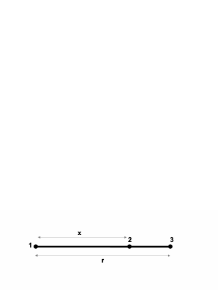
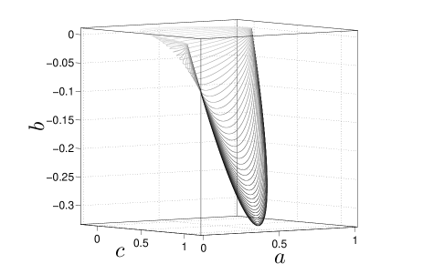
Figure 1: For 1-d configurations as specified in (a), the coefficients $a$ and $b$ are plotted versus $c$ in (b) at different values of the quantity $k_{F}x$. Plot traces change from black to light gray as $k_{F}x$ increases from 0.1 to 5.0 in steps of 0.1. For $k_{F}r\geq 4.5$, three $p$ functions attain positive values, placing the configuration outside the regime of genuine tripartite entanglement.

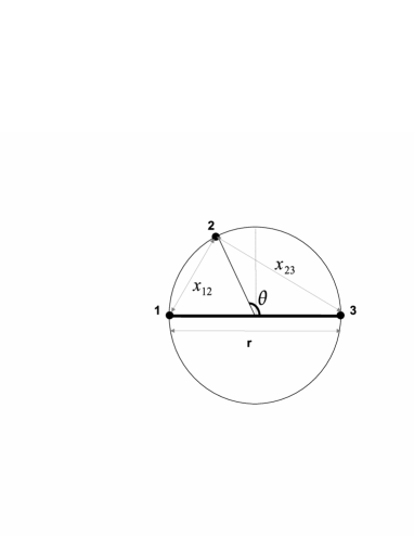
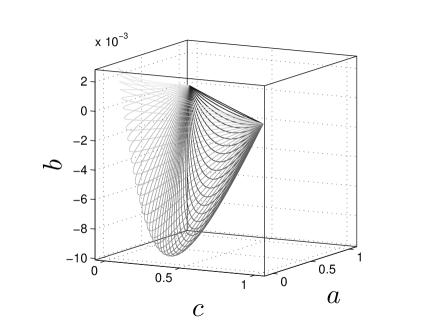
Figure 2: For 2-d configurations as specified in (a), the coefficients $a$ and $b$ are plotted versus $c$ in (b) at different values of $k_{F}x$. Particle 2 is considered to move on a circle of fixed radius $r$, with $x_{12}=r\cos{(\theta/2)}$ and $x_{23}=r\sin{(\theta/2)}$. The behavior of the coefficients is shown with traces changing from black to light gray as $k_{F}r$ increases from 0.1 to 5.0 in steps of 0.1.

III Entanglement Witnesses

The existence of an entanglement witness (EW) for any type of entangled state follows from the Hahn-Banach theorem rudin1 . In essence, this theorem establishes that if $C_{1}$ and $C_{2}$ are convex closed sets in a real Banach space, one of them being compact, there exists a bounded functional (identified here as the witness operator) that serves to separate the two sets. For example, an EW can be defined for entanglement class $e$ as an Hermitian operator $\mathcal{W}$ such that (a) $\mathrm{Tr}(\mathcal{W}\rho_{s})\geq 0$ for all fully separable states $\rho_{s}$ and (b) there exists at least one entangled state $\rho_{e}$ which can be detected by the condition $\mathrm{Tr}(\mathcal{W}\rho_{e})<0$. It will be relevant to later developments that this definition in itself cannot distinguish between different kinds of entanglement for more than bipartite systems.

The objective of the present work is the elucidation of the tripartite entanglement properties of the NIFG. This objective is pursued within the framework of the comprehensive analysis and classification of mixed three-qubit states provided by Acín et al. Acin . This classification is a generalization of that for pure three-qubit states. To introduce the necessary definitions and results, we first recall that the most general pure three-qubit state takes the form

$$|\psi_{GHZ}\rangle= \lambda_{0}|000\rangle+\lambda_{1}e^{i\theta}|100\rangle+\lambda_{2}|101\rangle$$

$$+\lambda_{3}|110\rangle+\lambda_{4}|111\rangle,$$ (22)

with $\lambda_{i}\geq 0$, $\sum_{i}\lambda_{i}^{2}=1$, and $\theta\in[0,\pi]$. For the three-qubit system, there are two types of locally inequivalent entangled pure states. These are the $GHZ$ type, defined by the form (III) with nontrivial parameters (especially, $\lambda_{4}>0$), and the $W$ type, represented generically by

$$|\psi_{W}\rangle=\lambda_{0}|000\rangle+\lambda_{1}|100\rangle+\lambda_{2}|101\rangle+\lambda_{3}|110\rangle.$$ (23)

The analysis of Ref. Acin, identifies four distinct classes of mixed three-qubit states. The corresponding sets, denoted by $S$, $B$, $W$, and $GHZ$, are all convex and compact, each being formed as a convex sum of appropriate projectors. Specifically, $S$ states are mixtures of product vectors; $B$ states are mixtures of product and biseparable vectors; $W$ states in turn are mixtures of product vectors, biseparable states, and $W$ vectors (23); and $GHZ$ states are mixtures of all of the previous vector types as well as $GHZ$ vectors (23). These four sets are invariant under local unitary and invertible non-unitary transformations. Evidently, they are nested according to $S\subset B\subset W\subset GHZ$.

Our development will also involve non-convex subsets such as $B\setminus S$, $W\setminus S$, $W\setminus B$, $GHZ\setminus S$, $GHZ\setminus B$, and $GHZ\setminus W$, which exclude fully separable states and hence contain only entangled states. A three-qubit state is said to possess genuine tripartite entanglement if it does not belong to the class of biseparable states $B$; such a state resides either in $GHZ\setminus W$ or $W\setminus B$.

The classification of mixed 3-qubit states introduced by Acín et al. Acin allows for the construction of entanglement witnesses—namely $GHZ$ EWs and $W$ EWs—that are capable of detecting states with genuine tripartite entanglement. Thus, $W$ EW will denote an operator $\mathcal{W}_{W}$ such that $\mathrm{Tr}(\mathcal{W}_{W}\rho_{B})\geq 0$ holds $\forall\rho_{B}\in B$, but for which there exists a $\rho_{GHZ\setminus B}\in GHZ\setminus B$ such that $\mathrm{Tr}(\mathcal{W}_{W}\rho_{GHZ\setminus B})<0$, thereby discriminating between the sets $B$ and $GHZ\setminus B$. Similarly, a $GHZ$ EW is provided by an operator $\mathcal{W}_{GHZ}$ such that $\mathrm{Tr}(\mathcal{W}_{GHZ}\rho_{W})\geq 0$ is satisfied for any $W$ state, but produces a negative expectation value for some $GHZ\setminus W$ state. Additionally, genuine tripartite entangled states, belonging to $GHZ\setminus W$ and $W\setminus B$, can be identified by means of an EW operator designed to detect $W\setminus B$ entanglement—as will be demonstrated in the next section.

A general scheme utilizing linear programming (LP) to arrive at EW operators for the detection of $GHZ\setminus S$ entangled states was introduced in Refs. hes1, ; hes2, . To confirm the presence of genuine tripartite entanglement in the NIFG one needs $W$ or $GHZ$ EWs. Construction of parameterized $GHZ$ EWs via the linear programming algorithm proceeds as follows. First, consider an Hermitian operator $\mathcal{W}$ in the form

$$\mathcal{W}=\sum_{i}a_{i}\widehat{P}_{i},$$ (24)

possessing at least one negative eigenvalue, where the $\widehat{P}_{i}$’s are Hermitian linear operators such that $x\leq\mathrm{Tr}(\widehat{P}_{i}\rho_{W})\leq y$ for all $x,y\in\mathbb{R}$ and for any density operator $\rho_{W}\in W$. The parameters $a_{i}\in\mathbb{R}$ are to be determined such that $\mathcal{W}$ qualifies as a $GHZ$ EW. As $\rho_{W}$ varies over $W$ states, $P^{W}_{i}=\mathrm{Tr}(\widehat{P}_{i}\rho_{W})$ maps $W$ states into a convex region, since a linear functional maps a convex domain (here, the $W$ class) to a convex region. Our principal task is to choose proper operators $\widehat{P}_{i}$ so as to obtain an approximating convex polyhedron surrounding the convex region spanned by the $P^{W}_{i}$ (the so-called feasible region for the LP optimization). The term “approximating” refers to the fact that in general, not all points in the convex polyhedron are produced by the expectation values of the $\widehat{P}_{i}$’s over $W$ states. By using this approximating convex polyhedron, the expectation value of the operator $\mathcal{W}$ over all $W$ states is non-negative and, with respect to other states, admits at least one negative value. Accordingly, in seeking to determine a $GHZ$ EWs of type (24), one needs to find the minimum expectation value of $\sum_{i}a_{i}P^{W}_{i}$ over the feasible region. In this way, the problem is reduced to optimization of the linear function $\sum_{i}a_{i}P^{W}_{i}$ over the convex set provided by the approximating convex polyhedron.

In characterizing the properties of the density operator for the NIFG, it is of interest to investigate the possibility of positive-partial transpose (PPT) entanglement, specifically the presence of a PPT entangled state with respect to some bipartition of a three-particle subsystem. The decomposability or non-decomposability of an EW may depend on which particles are involved. By definition, an EW $\mathcal{W}$ is partially decomposable with respect to the $i$-th party iff there exist positive operators $\widehat{P},\widehat{Q}$ such that $\mathcal{W}=\widehat{P}+\widehat{Q}^{T_{i}}$, where $i\in\{1,2,3\}$ and $T_{i}$ stands for partial transposition with respect to $i$-th party. Accordingly, an EW is called partially non-decomposable EW with respect to a given party iff there exists at least one PPT entangled state associated with that party, i.e., $\rho^{T_{i}}\geq 0$ when $\mathrm{Tr}(\mathcal{W}\rho)<0$. The relevance of these definitions will become clear when we encounter EWs that must explicitly bear the label of the party (or particle) with respect to which it is decomposable. For the purpose of identifying a PPT state with respect to a given party, one may derive the following conditions for the parameters in $\rho_{3}$: A positive value for $\rho^{T_{1}}$ requires

$$a^{2}+b^{2}+c^{2}+ac+bc-ab\geq 0,$$

$$2(a^{2}+b^{2}+c^{2}+ac+bc-ab)^{1/2}-1\leq-a-b+c\leq 1,$$ (25)

the condition $\rho^{T_{2}}\geq 0$ is met only if

$$a^{2}+b^{2}+c^{2}-ac+bc+ab\geq 0,$$

$$2(a^{2}+b^{2}+c^{2}-ac+bc+ab)^{1/2}-1\leq-a+b-c\leq 1,$$ (26)

and $\rho^{T_{3}}\geq 0$ implies

$$a^{2}+b^{2}+c^{2}+ac-bc+ab\geq 0,$$

$$2(a^{2}+b^{2}+c^{2}+ac-bc+ab)^{1/2}-1\leq a-b-c\leq 1.$$ (27)

The presence of a PPT entangled density matrix with respect to a given party is signaled by satisfaction the corresponding necessary condition among (III-27) together with its detection by the corresponding EW operator. Evidently, only a partially non-decomposable EW related to the selected party can detect a PPT entangled state with respect to that party.

IV EW operators for the NIFG

In accordance with the strategy proposed in Ref. hes2, , we now apply the LP method to determine proper EW operators for identification of chosen entanglement classes in the density matrix of the NIFG. We first consider EW construction based on an extended spin-chain model, and then build a new class of $GHZ$ EWs from an appropriate set of density operators. Finally, we utilize stabilizer operators to develop EWs that discriminate between different classes of genuine tripartite entanglement.

IV.1 Spin-chain model

Gühne et al. Guh1 were the first to introduce an EW operator ($W$ EW) to detect genuine tripartite entanglement based on a macroscopic spin-chain model. The explicit form of this EW is

$$\mathcal{W}^{({\rm gen})}=(1+\sqrt{5})\textbf{I}+\widehat{P}_{12}+\widehat{P}_{23},$$ (28)

where $\widehat{P}_{ij}=\sigma^{(i)}\cdot\sigma^{(j)}$, or more rigorously

$$\widehat{P}_{12}= \sigma^{(1)}\cdot\sigma^{(2)}$$

$$= \sigma_{x}^{(1)}\sigma_{x}^{(2)}\textbf{I}^{(3)}+\sigma_{y}^{(1)}\sigma_{y}^{(2)}\textbf{I}^{(3)}+\sigma_{z}^{(1)}\sigma_{z}^{(2)}\textbf{I}^{(3)},$$

$$\widehat{P}_{23}= \sigma^{(2)}\cdot\sigma^{(3)}$$

$$= \textbf{I}^{(1)}\sigma_{x}^{(2)}\sigma_{x}^{(3)}+\textbf{I}^{(1)}\sigma_{y}^{(2)}\sigma_{y}^{(3)}+\textbf{I}^{(1)}\sigma_{z}^{(2)}\sigma_{z}^{(3)}.$$ (29)

The superscripts identify the parties involved and $\sigma=(\sigma_{x},\sigma_{y},\sigma_{z})$. As required, the operator $\mathcal{W}^{({\rm gen})}$ has positive expectation values with respect to all states belonging to $B$ and has a negative expectation value with respect to some genuine tripartite entangled state in $GHZ\setminus B$.

Implementing the EW of Gühne et al. Guh1 , Vértesi Vert1 has shown that in a particular three-fermion configuration, there exists genuine tripartite entanglement in the NIFG. Our goal is to identify the type of genuine tripartite entanglement present in the NIFG. We develop EW operators suitable for this system and seek boundary conditions for separated fermions exploiting the witness operators.

Starting from spin-chain model used in Ref. Guh1, to construct the EW of Eq. (28), we consider the operator

$$\mathcal{W}_{1}=c_{0}\;\textbf{I}+\widehat{P}_{12}+\widehat{P}_{23}$$ (30)

and ask whether the constant $c_{0}$ can be chosen so that $\mathcal{W}_{1}$ becomes a $GHZ$ EW. To answer this question, we should find the minimum expectation value of $\widehat{P}_{12}+\widehat{P}_{23}$ over all states in $W$ set. The domain of $W$ states is spanned by the explicit general form (23) for $|\psi_{W}\rangle$, subject to any local $SU(2)$ transformation. Upon expanding such the general $W$ vector as $|\Psi_{W}\rangle=\sum_{i,j,k=0,1}A_{ijk}|ijk\rangle$, one can evaluate the coefficient $A_{ijk}$ and thus the expectation values $P_{ij}^{W}=\langle\Psi_{W}|P_{ij}|\Psi_{W}\rangle$. (See the appendix for details.) It is then easily seen that the witness $\mathcal{W}_{1}$ can only detect $W\setminus B$ states, since the eigenvector associated with the minimum eigenvalue $-4$ of $\widehat{P}_{12}+\widehat{P}_{23}$ belongs to $W$ domain, so $\mathcal{W}_{1}$ can never be a $GHZ$ EW.

Evaluating the expectation value of (28) with respect to $\rho_{3}$, we obtain

$$\mathrm{Tr}(\mathcal{W}^{({\rm gen})}\rho_{3})=1+\sqrt{5}-3(a+c),$$ (31)

which cannot be negative and maintain the condition $a+b+c<1$ specific to the NIFG.

To investigate the existence of genuine tripartite entanglement, we adopt the more general form

$$\rho_{3}^{\prime}=U\rho_{3}U^{{\dagger}}$$ (32)

for the density operator, where

$$U=\left(\begin{array}[]{cc}\beta^{*}&\alpha\\ -\alpha^{*}&\beta\\ \end{array}\right)^{\otimes 3}$$ (33)

performs an arbitrary local unitary transformation of the density operator $\rho_{3}$ of the NIFG. (The same transformation is applied for all three fermions, with $|\alpha|^{2}+|\beta|^{2}=1$.) We then find

$$\mathrm{Tr}(\mathcal{W}^{({\rm gen})}\rho_{3}^{\prime})=1+\sqrt{5}+(2-2b-7a-7c)|\beta^{2}\alpha^{4}|$$

$$-9(a+c)|\alpha^{2}\beta^{4}|-(a+c)|\alpha|^{6}-3(a+c)|\beta|^{6}.$$ (34)

For one-dimensional configurations specified as in Fig. 1, Fig. 3 shows the value of $\mathrm{Tr}(\mathcal{W}^{({\rm gen})}\rho_{3}^{\prime})$ as a function of $k_{F}x$ for $k_{F}r=0.1$. It is seen that $W\setminus B$ entanglement is present over the range $0.01\leq k_{F}x\leq 0.09$.

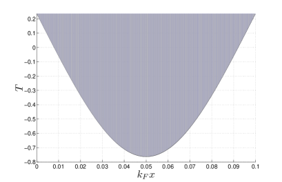
Figure 3: Plot of the expectation value $T=\mathrm{Tr}(\mathcal{W}^{({\rm gen})}\rho_{3}^{\prime})$ versus $k_{F}x$ at $k_{F}r=0.1$, in the 1-d coordinate scheme of Fig. 1. Here, $\mathcal{W}^{({\rm gen})}$ is the entanglement witness (28) and $\rho_{3}^{\prime}$ is the transform (32) of the three-fermion reduced density matrix $\rho_{3}$ under an arbitrary local unitary operator. Physically, the distance of particle 2 from particle 1 is varied while the distance between particles 1 and 3 is kept fixed. The trace $T$ lies inside the gray region when $k_{F}x$ varies between 0 and $k_{F}r$ and the parameters $\alpha$ and $\beta$ range over all allowed values.

Acknowledging the indistinguishability of the fermion constituents of the NIFG, we turn to a more general EW construction based on a parametrized operator that superposes all three of the spin products $\widehat{P}_{ij}$:

$$\mathcal{W}^{(\mathrm{sp})}=a_{0}\;\textbf{I}+a_{12}\widehat{P}_{12}+a_{13}\widehat{P}_{13}+a_{23}\widehat{P}_{23}.$$ (35)

For equal values of the real parameters $a_{12}=a_{13}=a_{23}$, $\mathcal{W}^{(\mathrm{sp})}$, this ansatz reduces to $\mathcal{W}^{(\mathrm{sp})}=a_{0}\mathbf{I}_{8}+a_{12}(\widehat{P}_{12}+\widehat{P}_{13}+\widehat{P}_{23})$ which resembles a spin-chain model with periodic boundary condition. We now consider the possibility that $\mathcal{W}^{(\mathrm{sp})}$ can provide a $W$ EW or even a $GHZ$ EW by examining the constraints on the parameters $a_{0}$, $a_{12}$, $a_{13}$, and $a_{23}$.

In establishing $\mathcal{W}^{(\mathrm{sp})}$ as a $W$ EW detecting genuine tripartite entanglement, the essential task is to find a convex polyhedron spanned by the $P^{B}_{ij}$, i.e., the expectation values of the $\widehat{P}_{ij}$ with respect to the $B$ class of states (as considered in the appendix). As a first conjecture delimiting the eigenvalues of the $\widehat{P}_{ij}$, we propose the set of inequalities

$$-3\leq P^{B}_{12},P^{B}_{13},P^{B}_{23}\leq 1,$$

$$-P^{B}_{12}-P^{B}_{13}+P^{B}_{23}\leq 3,$$

$$-P^{B}_{12}+P^{B}_{13}-P^{B}_{23}\leq 3,$$

$$P^{B}_{12}-P^{B}_{13}-P^{B}_{23}\leq 3.$$ (36)

The polyhedron so described does not encompass the region spanned by the $P^{B}_{ij}$. However, by parallel shifts of the boundaries in relations (IV.1), one can find a proper approximating convex polyhedron for reduction of the problem of finding a $W$ EW to one of linear programming. This step is outlined in the appendix. The resulting optimization problem reads:

$$\mathrm{Minimize}\quad\;\;a_{0}+a_{12}P^{B}_{12}+a_{13}P^{B}_{13}+a_{23}P^{B}_{23},$$

$$\mathrm{subject\ to}\quad\;\;\left\{\begin{array}[]{c}-3\leq P^{B}_{12},P^{B}_{13},P^{B}_{23}\leq 1,\\ -P^{B}_{12}-P^{B}_{13}+P^{B}_{23}\leq 1+\sqrt{8},\\ -P^{B}_{12}+P^{B}_{13}-P^{B}_{23}\leq 1+\sqrt{8},\\ P^{B}_{12}-P^{B}_{13}-P^{B}_{23}\leq 1+\sqrt{8}.\end{array}\right.$$ (41)

With regard to maximum eigenvalues, the expectation values of

$$\widehat{P}_{23}-\widehat{P}_{12}-\widehat{P}_{13},$$

$$\widehat{P}_{13}-\widehat{P}_{12}-\widehat{P}_{23},$$

$$\widehat{P}_{12}-\widehat{P}_{13}-\widehat{P}_{23}$$ (42)

reach 5. Therefore, solution of the LP problem (IV.1) determines a region in which to form $\mathcal{W}^{(\mathrm{sp})}$ as a witness operator. Solution proceeds by considering the intersection of the constraints expressed in (IV.1) and finding the vertices of the convex polyhedron. Upon solving the LP problem, one can obtain the values of the parameters $a_{0}$, $a_{12}$, $a_{13}$ and $a_{23}$ satisfying

$$a_{0}+(3-\sqrt{8})a_{12}-3a_{13}+a_{23}\geq 0,$$

$$a_{0}-3a_{12}+(3-\sqrt{8})a_{13}+a_{23}\geq 0,$$

$$a_{0}-3a_{12}-3a_{13}+(-5+\sqrt{8})a_{23}\geq 0,$$

$$a_{0}+(3-\sqrt{8})a_{12}+a_{13}-3a_{23}\geq 0,$$

$$a_{0}-3a_{12}+a_{13}+(3-\sqrt{8})a_{23}\geq 0,$$

$$a_{0}-3a_{12}+(-5+\sqrt{8})a_{13}-3a_{23}\geq 0,$$

$$a_{0}+a_{12}-3a_{13}+(3-\sqrt{8})a_{23}\geq 0,$$

$$a_{0}+a_{12}+(3-\sqrt{8})a_{13}-3a_{23}\geq 0,$$

$$a_{0}+(-5+\sqrt{8})a_{12}-3a_{13}-3a_{23}\geq 0,$$

$$a_{0}+a_{12}+a_{13}+a_{23}\geq 0,$$

$$a_{0}+a_{12}+a_{13}-3a_{23}\geq 0,$$

$$a_{0}-3a_{12}+a_{13}+a_{23}\geq 0,$$

$$a_{0}+a_{12}-3a_{13}+a_{23}\geq 0,$$

$$a_{0}-3a_{12}-3a_{13}-3a_{23}\geq 0,$$ (43)

provided that the expectation value of $\mathcal{W}^{(\mathrm{sp})}$ is positive for all quantum states in the $W$ set. Additionally, for $\mathcal{W}^{(\mathrm{sp})}$ to qualify as a $W$ EW, at least one of the eigenvalues $E_{i}$ among

$$E_{1} =a_{0}+a_{12}+a_{13}+a_{23},$$

$$E_{2,3} =a_{0}-a_{12}-a_{13}-a_{23}$$

$$\pm(a_{12}^{2}+a_{13}^{2}+a_{23}^{2}-a_{12}a_{13}-a_{12}a_{23}-a_{13}a_{23})^{1/2},$$ (44)

must be negative, i.e., $\mathrm{min}(E_{i})<0$ for $i=1,2,3$, thus imposing on the parameters $a_{i}$ a condition additional to those of Eq. (IV.1).

In order to distinguish between different classes of genuine tripartite entanglement, one would like to find a set of parameters such that $\mathcal{W}^{(\mathrm{sp})}$ becomes a $GHZ$ EW. Following the same pattern as above, we seek a proper polyhedron spanned by the $P^{W}_{ij}$ (see appendix, Eq. (A-5)). It is found that the maximum value of $-P^{W}_{12}-P^{W}_{13}+P^{W}_{23}$, $-P^{W}_{12}+P^{W}_{13}-P^{W}_{23}$, and $P^{W}_{12}-P^{W}_{13}-P^{W}_{23}$ reaches $5$, which is the maximum eigenvalue of the operators in Eqs. (IV.1). Hence $\mathcal{W}^{(\mathrm{sp})}$ can never be a $GHZ$ EW for any choice of the parameters $a_{i}$. It may be noted that use of the form $\mathcal{W}^{(\mathrm{sp})}$ in construction of an EW operator is compatible with the idea of developing it in terms of the projection operators $|\Psi_{ij}^{-}\rangle\langle\Psi_{ij}^{-}|\otimes\textbf{I}^{(k)}$ present in the expansion (II) of $\rho_{3}$, since one can write

$$|\Psi_{ij}^{-}\rangle\langle\Psi_{ij}^{-}|\otimes\textbf{I}^{(k)}=\frac{1}{4}(\textbf{I}-\sigma^{(i)}\cdot\sigma^{(j)}).$$ (45)

However, the more general (and more successful) implementation of this idea pursued in Sec. IV.2 takes into account projectors referring to the set $GHZ\setminus B$.

Returning to the task of detecting genuine tripartite entanglement in the three-particle reduced density matrix of the NIFG, we try $W$ EWs corresponding to the ansatz

$$^{0}\mathcal{W}_{W}^{(\mathrm{sp})}=(1+\sqrt{8})\;\textbf{I}+\widehat{P}_{12}+\widehat{P}_{13}-\widehat{P}_{23}.$$ (46)

For the trace of the product of ${}^{0}\mathcal{W}_{W}^{(\mathrm{sp})}$ with $\rho_{3}$ we obtain

$$\mathrm{Tr}(^{0}\mathcal{W}_{W}^{(\mathrm{sp})}\rho_{3})=(1+\sqrt{8})-3(a+b-c),$$ (47)

which must be negative to signal the existence of $W\setminus B$ entanglement in $\rho_{3}$. For the NIFG the maximum value of $a+b-c$ is $1$. It can then be checked that the constraints imposed on the coefficients $a$, $b$, and $c$ for the NIFG exclude the possibility of a negative expectation value of ${}^{0}\mathcal{W}_{W}^{(\mathrm{sp})}$ for the NIFG density matrix operator. We are led to conclude that symmetric spin-chain EWs are not capable of detecting genuine tripartite entanglement in NIFG.

On the other hand, if we consider the general case of a density-matrix operator of the form (II) subject to the basic constraints (II), but not specializing to the NIFG, the expectation value of ${}^{0}\mathcal{W}_{W}^{(\mathrm{sp})}$ over $\rho_{3}$ can take on a negative value for some set of parameter values. It should be emphasized that entanglement detected by ${}^{0}\mathcal{W}_{W}^{(\mathrm{sp})}$ in such a general density matrix $\rho_{3}$ necessarily belongs to the $W\setminus B$ class rather than the other class of genuine tripartite entanglement, i.e., $GHZ\setminus W$. We note that in the case of the transformed density matrix $\rho_{3}^{\prime}$ introduced in Eq. (32), the relation

$$\mathrm{Tr}(^{0}\mathcal{W}_{W}^{(\mathrm{sp})}\rho_{3}^{\prime})= (1+\sqrt{8})+(-a-3b+c)|\alpha|^{6}$$

$$+(-3a-3b+3c)|\beta|^{6}$$

$$+(-8a-9b+6c)|\alpha^{4}\beta^{2}|$$

$$+(-9a-9b+9c)|\alpha^{2}\beta^{4}|<0$$ (48)

must be satisfied for $W\setminus B$ identification.

Having explored periodic spin-chain models for EW operators, we next describe another approach to the problem of constructing EWs for the NIFG via LP, based on projection operators making up the density matrix $\rho_{3}$ in Eq. (II).

IV.2 $GHZ$ EWs composed of projection operators

In this section, we develop a new class of proper $GHZ$ EWs with the aid of projection operators (pure-state density matrices) corresponding to the different entangled density operators arising in tripartite systems. If an EW is to detect tripartite entanglement associated with a given class of biseparables (1-23, 2-13, or 3-12), or with genuine entangled states ($W\setminus B$ or $GHZ\setminus W$), it must necessarily be constructed from operators having non-vanishing expectation value with respect to the class that is specified. In particular, as demonstrated in the Sec. IV.1 (see e.g., Eq. (45)), a $GHZ$ EW cannot be successfully built from projection operators of the $GHZ$ set if projectors from the $GHZ\setminus W$ class are excluded.

With this preface, we introduce the operator

$$\mathcal{W}_{GHZ}^{d}=a_{0}\textbf{I}_{8}$$

$$+a_{1}(|\Psi_{12}^{-}\rangle\langle\Psi_{12}^{-}|\otimes\textbf{I}+|\Psi_{13}^{-}\rangle\langle\Psi_{13}^{-}|\otimes\textbf{I}+\textbf{I}\otimes|\Psi_{23}^{-}\rangle\langle\Psi_{23}^{-}|)$$

$$+a_{2}|W_{1}\rangle\langle W_{1}|+a_{3}|W_{2}\rangle\langle W_{2}|+a_{4}|\Psi_{123}^{-}\rangle\langle\Psi_{123}^{-}|,$$ (49)

which contains projection operators for all the different vector types involved for the three-fermion subsystem,

$$|W_{1}\rangle=\frac{1}{\sqrt{3}}(|001\rangle+|010\rangle+|100\rangle),$$

$$|W_{2}\rangle=\frac{1}{\sqrt{3}}(|011\rangle+|110\rangle+|101\rangle),$$

$$|\Psi_{123}^{-}\rangle=\frac{1}{\sqrt{2}}(|000\rangle-|111\rangle),$$ (50)

and the $a_{i}$ are real parameters. First, to ensure that the operator (IV.2) qualifies as a $GHZ$ EW, we should impose positivity of the expectation value of $\mathcal{W}_{GHZ}^{d}$ with respect to $W$ states. We take the generic $W$ state vector $|\Psi_{W}\rangle$ in the form (23). For simplicity we define the operators

$$\widehat{P}_{1}:=2\sum_{<i,j>}|\Psi_{ij}^{-}\rangle\langle\Psi_{ij}^{-}|\otimes\textbf{I},$$

$$\widehat{P}_{2}:=3|W_{1}\rangle\langle W_{1}|,\quad\widehat{P}_{3}:=3|W_{2}\rangle\langle W_{2}|,$$

$$\widehat{P}_{4}:=2|\Psi_{123}^{-}\rangle\langle\Psi_{123}^{-}|,$$ (51)

and therewith their corresponding expectation values $P_{i}^{W}$ ($i=1,2,3,4$) with respect to $W$-vectors in terms of the coefficients $A_{ijk}$ explicated in the appendix. One readily finds that the maximum eigenvalue is 3 for $\widehat{P}_{1}$, $\widehat{P}_{2}$, and $\widehat{P}_{3}$ and 2 for $\widehat{P}_{4}$. A straightforward calculation shows that $P^{W}_{1}$, $P^{W}_{2}$, and $P^{W}_{3}$ can reach their maximum possible value, but for $P^{W}_{4}$ one finds a maximum overlap $\langle\Psi_{123}^{-}|\psi_{W}\rangle$ of $3/2$.

To reduce the task of determining parameter values $a_{i}$ such that $\mathcal{W}_{GHZ}^{d}$ becomes a $GHZ$ EW operator to an LP problem, we need to find a feasible region. Basing a first conjecture on the maximum eigenvalues of the $\widehat{P}_{i}$ we find that the extremum points

$$(P^{W}_{1},P^{W}_{2},P^{W}_{3},P^{W}_{4})= (0,0,0,0),(3,0,0,0),(0,3,0,0),$$

$$(0,0,3,0),(0,0,0,3/2)$$ (52)

cannot be vertices for a feasible region of our LP problem. As checked numerically, some points lying outside the convex polyhedron with vertices specified by (IV.2) correspond to negative expectation values for $\mathcal{W}_{GHZ}^{d}$. To compensate, we extend the proposed region by a parallel shift of the boundary hyperplane and reduce the problem to LP as follows:

$$\mathrm{Minimize}\quad\;\;a_{0}+\sum_{i=1}^{4}a_{i}P^{W}_{i}$$

$$\mathrm{subject\ to}\quad\;\;\left\{\begin{array}[]{c}0\leq P^{W}_{1},P^{W}_{2},P^{W}_{3}\leq 3,\\ 0\leq P^{W}_{4}\leq 2,\\ 0\leq P^{W}_{1}+P^{W}_{2}+P^{W}_{3}+2P^{W}_{4}\leq\frac{15}{4}.\\ \end{array}\right.$$ (56)

Imposing the latter constraints, the operator $\mathcal{W}_{GHZ}^{d}$ can still have one or more negative expectation values since the range of the expectation value of $\widehat{P}_{1}+\widehat{P}_{2}+\widehat{P}_{3}+2\widehat{P}_{4}$ is bounded between 0 and 4. Now we have a feasible region formed by the intersection of the 4-dimensional rectangular parallelepiped domain defined by the extremum eigenvalues of the $\widehat{P}_{i}$’s and the constraining hyperplane $P^{W}_{1}+P^{W}_{2}+P^{W}_{3}+2P^{W}_{4}\leq 15/4$. We illustrate the situation in Fig. 4, projecting onto the $P^{W}_{1}$ dimension.

The resulting convex polyhedron has vertices

$$(P^{W}_{1},P^{W}_{2},P^{W}_{3},P^{W}_{4})= (0,0,0,0),(3,0,0,0),(3,0,0,3/8),(3,0,3/4,0),$$ (57)

$$(3,3/4,0,0),(0,3,0,0),(0,3,0,3/8),(0,3,3/4,0),(3/4,3,0,0),$$

$$(0,0,3,0),(0,0,3,3/8),(0,3/4,3,0),(3/4,0,3,0),(0,0,0,15/8).$$

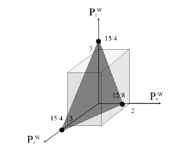
Figure 4: Projection of the feasible region of the LP problem on the $P^{W}_{1}$ dimension, showing the intersection domain of the region $P^{W}_{2}+P^{W}_{3}+2P^{W}_{4}\leq 15/4$ and the domain of possible expectation values of $\widehat{P}_{2},\widehat{P}_{3},\widehat{P}_{4}$ with respect to a generic tripartite quantum state within the rectangular parallelepiped.

After solving the LP problem posed in (IV.2), we arrive at a set of the $a_{i}$,

$$a_{0}\geq 0,\;a_{0}+3a_{1}\geq 0,\;a_{0}+3a_{2}\geq 0,\;a_{0}+3a_{3}\geq 0,\;a_{0}+15a_{4}/8\geq 0,$$

$$a_{0}+3a_{1}+3a_{4}/8\geq 0,\;a_{0}+3a_{2}+3a_{4}/8\geq 0,\;a_{0}+3a_{3}+3a_{4}/8\geq 0,$$

$$a_{0}+3a_{1}+3a_{2}/\geq 0,\;a_{0}+3a_{1}+3a_{3}/4\geq 0,\;a_{0}+3a_{2}+3a_{3}/4\geq 0,$$

$$a_{0}+3a_{2}+3a_{1}/4\geq 0,\;a_{0}+3a_{3}+3a_{1}/4\geq 0,\;a_{0}+3a_{3}+3a_{2}/4\geq 0,$$ (58)

imposed by the positivity of the trace of of the EW operator over all $W$ states. These constraints, together with the existence of at least one negative eigenvalue among

$$a_{o},a_{0}+3a_{1},a_{0}+3a_{2},a_{0}+3a_{3},a_{0}+2a_{4},$$ (59)

guarantee that $\mathcal{W}_{GHZ}^{d}$ qualifies as a $GHZ$ EW. Among the combinations (59), only $a_{0}$ is excluded from negativity, with the others remaining available for signaling a $GHZ\setminus W$ state.

We are now prepared to search for $GHZ\setminus W$ genuine entanglement in the NIFG. As an optimal case of our $GHZ$ EW construction, the inequality in Eq. (IV.2) specifying the last boundary hyperplane of the present LP problem yields the explicit $GHZ$ EW operator

$$^{0}\mathcal{W}_{GHZ}^{d}= \frac{15}{4}\textbf{I}_{8}-2\sum_{<i,j>}|\Psi_{ij}^{-}\rangle\langle\Psi_{ij}^{-}|-3|W_{1}\rangle\langle W_{1}|$$

$$-3|W_{2}\rangle\langle W_{2}|-4|\Psi_{123}^{-}\rangle\langle\Psi_{123}^{-}|.$$ (60)

Adopting the witness ${}^{0}\mathcal{W}_{GHZ}^{d}$ for our search, we calculate its expectation value for the three-fermion reduced density matrix $\rho_{3}$ of the NIFG, obtaining the simple expression

$$\mathrm{Tr}(^{0}\mathcal{W}_{GHZ}^{d}\rho_{3})=\frac{1}{2}+2\eta,$$ (61)

which would have to be negative to confirm the presence of $GHZ\setminus W$ entanglement. However, as seen in Fig. 6, the term $\eta$ does not reach negative values, ruling out this possibility. Moreover, calculation of the expectation value of the best-case witness operator $\mathcal{W}_{GHZ}^{d}$ with respect to the rotated three-fermion reduced density matrix of Eq. (32) yields

$$\mathrm{Tr}(^{0}\mathcal{W}_{GHZ}^{d}\rho_{3}^{\prime})=\frac{15}{4}$$

$$+\left(\frac{|\alpha^{4}\beta^{2}|}{4}+\frac{|\alpha^{2}\beta^{4}|}{4}\right)\left(-33+9a-3b+9c\right)$$

$$-\left(\frac{|\alpha|^{6}}{4}+\frac{|\beta|^{6}}{4}\right)\left(11+a+b+c\right)$$

$$+\left(\frac{\alpha^{*3}\beta^{3}}{2}+\frac{\beta^{*3}\alpha^{3}}{2}\right)(1-a-b-c),$$ (62)

which again fails to attain negative values.

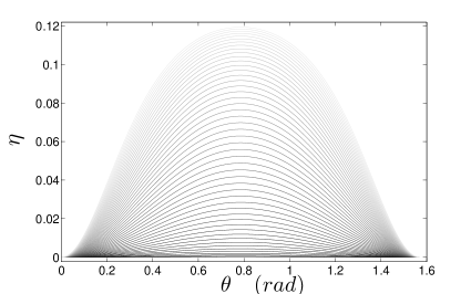
Figure 5: Plots of the term $\eta$ in Eq. (61) versus $\theta$ (in radians) at different values of $k_{F}r$ for the 2-d configuration shown in Fig. 2. (Plot traces change from black to light gray as $k_{F}$ is increased from 0.1 to 5.0 in steps of 0.1.)

In the next subsection, $GHZ$ stabilizer operators will be employed to formulate still another class of entanglement witnesses.

IV.3 Stabilizer EWs

Previous work has demonstrated the utility and robustness of EWs based on stabilization operators Gottes ; Toth1 ; Toth2 ; hes2 . By definition a stabilizer operator ${\hat{S}}$ for state $|\psi\rangle$ has the property ${\hat{S}}|\psi\rangle=|\psi\rangle$. Tóth and Gühne Toth1 ; Toth2 have shown that if some of the stabilizing operators for a given state are available, entanglement conditions may be found that detect states in the neighborhood of this state. Here we apply the stabilizer formalism to obtain a parameterized EW for detecting quantum states close to a $GHZ$ entangled state. Also employing stabilizer operators, we are able to discriminate between different types of genuine tripartite entanglement that could be present in the three-particle reduced density matrix.

We begin by considering a linear combination

$$\mathcal{W}^{({\rm stab})}=b_{0}\textbf{I}+b_{1}\widehat{S}_{1}+b_{2}\widehat{S}_{2}+b_{1,2}\widehat{S}_{1,2}$$ (63)

of $GHZ$ stabilizer operators $\widehat{S}_{1}=\sigma^{(1)}_{x}\sigma^{(2)}_{x}\sigma^{(3)}_{x}$, $\widehat{S}_{2}=\sigma^{(1)}_{z}\sigma^{(2)}_{z}\textbf{I}^{(3)}$, and $\widehat{S}_{1,2}=\widehat{S}_{1}\times\widehat{S}_{2}$, where the $b_{i}$’s are real parameters. First, to find ranges of the parameters $b_{i}$ such that $\mathcal{W}^{({\rm stab})}$ becomes a $W$ EW, we must determine the domain spanned by the expectation values $S^{B}_{i}$ of the corresponding operators $\widehat{S}_{i}$ over the biseparable set of states. Straightforward calculation shows that this task can be reduced to the solution of the following LP problem (see the appendix):

$$\mathrm{Minimize}\quad\;\;b_{0}+b_{1}S^{B}_{1}+b_{2}S^{B}_{2}+b_{12}S^{B}_{12}$$

$$\mathrm{subject\ to}\quad\;\;\left\{\begin{array}[]{cc}\begin{array}[]{c}(-1)^{i_{1}}S^{B}_{1}+(-1)^{i_{2}}S^{B}_{2}+(-1)^{i_{1}+i_{2}}S^{B}_{1,2}\leq\sqrt{2},\\ (-1)^{i_{1}}S^{B}_{1}+(-1)^{i_{2}}S^{B}_{2}+(-1)^{i_{1}+i_{2}+1}S^{B}_{1,2}\leq 1,\end{array}&\;\;\;\;\forall(i_{1},i_{2})\in\{0,1\}^{2}.\end{array}\right.$$ (67)

It is to be noted here that the boundaries associated with separable states cannot exceed unity hes2 . The operators corresponding to the second set of constraints in (IV.3), i.e.,

$$(-1)^{i_{1}}\widehat{S}_{1}+(-1)^{i_{2}}\widehat{S}_{2}+(-1)^{i_{1}+i_{2}+1}\widehat{S}_{1,2},\quad(i_{1},i_{2})\in\{0,1\},$$ (68)

are positive operators and thus cannot form EW operators. In solving the LP problem stated in (IV.3), we find that the constraints

$$\begin{array}[]{cc}b_{0}+\sqrt{2}(b_{1}+b_{2}-b_{1,2})\geq 0,&b_{0}+\sqrt{2}(b_{1}-b_{2}+b_{1,2})\geq 0,\\ b_{0}+\sqrt{2}(-b_{1}+b_{2}+b_{1,2})\geq 0,&b_{0}-\sqrt{2}(b_{1}+b_{2}+b_{1,2})\geq 0,\\ b_{0}+b_{1}-b_{2}-b_{1,2}\geq 0,&b_{0}-b_{1}-b_{2}+b_{1,2}\geq 0,\\ b_{0}-b_{1}+b_{2}-b_{1,2}\geq 0,&b_{0}+b_{1}+b_{2}+b_{1,2}\geq 0\\ b_{0}+\sqrt{2}b_{1}+\frac{1-\sqrt{2}}{2}b_{2}+\frac{-1+\sqrt{2}}{2}b_{1,2}\geq 0,&b_{0}+\sqrt{2}b_{1}+\frac{-1+\sqrt{2}}{2}b_{2}+\frac{1-\sqrt{2}}{2}b_{1,2}\geq 0,\\ b_{0}+\frac{-1+\sqrt{2}}{2}b_{1}+\sqrt{2}b_{2}+\frac{1-\sqrt{2}}{2}b_{1,2}\geq 0,&b_{0}+\frac{1-\sqrt{2}}{2}b_{1}+\sqrt{2}b_{2}+\frac{-1+\sqrt{2}}{2}b_{1,2}\geq 0,\\ b_{0}+\frac{-1+\sqrt{2}}{2}b_{1}+\frac{1-\sqrt{2}}{2}b_{2}+\sqrt{2}b_{1,2}\geq 0,&b_{0}+\frac{-1+\sqrt{2}}{2}b_{1}+\frac{1-\sqrt{2}}{2}b_{2}+\sqrt{2}b_{1,2}\geq 0,\\ b_{0}+\frac{1-\sqrt{2}}{2}b_{1}+\frac{1-\sqrt{2}}{2}b_{2}-\sqrt{2}b_{1,2}\geq 0,&b_{0}+\frac{-1+\sqrt{2}}{2}b_{1}+\frac{-1+\sqrt{2}}{2}b_{2}-\sqrt{2}b_{1,2}\geq 0,\\ b_{0}+\frac{1-\sqrt{2}}{2}b_{1}-\sqrt{2}b_{2}+\frac{1-\sqrt{2}}{2}b_{1,2}\geq 0,&b_{0}+\frac{-1+\sqrt{2}}{2}b_{1}-\sqrt{2}b_{2}+\frac{-1+\sqrt{2}}{2}b_{1,2}\geq 0,\\ b_{0}-\sqrt{2}b_{1}+\frac{1-\sqrt{2}}{2}b_{2}+\frac{1-\sqrt{2}}{2}b_{1,2}\geq 0,&b_{0}-\sqrt{2}b_{1}+\frac{-1+\sqrt{2}}{2}b_{2}+\frac{-1+\sqrt{2}}{2}b_{1,2}\geq 0\\ \end{array}$$ (69)

guarantee positivity of $\mathcal{W}^{({\rm stab})}$ over all biseparable states. However, for $\mathcal{W}^{({\rm stab})}$ to qualify as the $W$ EW we seek, it also must possess at least one negative eigenvalue from the possibilities

$$b_{0}+(-1)^{i_{1}}b_{1}+(-1)^{i_{2}}b_{2}+(-1)^{i_{1}+i_{2}}b_{1,2},\quad\forall(i_{1},i_{2})\in\{0,1\}^{2}$$ (70)

Next, to enable discrimination between different kinds of genuine entangled states, a $GHZ$ EW is required. Accordingly, we should find values of the $b$ coefficients in Eq. (63) such that $\mathcal{W}^{({\rm stab})}$ is positive over all the states in the $W$ class and yet has at least one negative eigenvalue. To this end, we search for a polyhedron spanned by the expectation values $S^{W}_{1}$, $S^{W}_{2}$, and $S^{W}_{1,2}$, which are functions of the coefficients $A_{ijk}$ in the general $W$ vector $|\Psi_{W}\rangle$ as expressed previously. Following the same pattern as before, we are led to the LP problem

$$\mathrm{Minimize}\quad\;\;b_{0}+b_{1}S^{W}_{1}+b_{2}S^{W}_{2}+b_{12}S^{W}_{12}$$

$$\mathrm{subject\ to}\quad\;\;\left\{\begin{array}[]{cc}\begin{array}[]{c}(-1)^{i_{1}}S^{W}_{1}+(-1)^{i_{2}}S^{W}_{2}+(-1)^{i_{1}+i_{2}}S^{W}_{1,2}\leq 2.98\\ (-1)^{i_{1}}S^{W}_{1}+(-1)^{i_{2}}S^{W}_{2}+(-1)^{i_{1}+i_{2}+1}S^{W}_{1,2}\leq 1\end{array}&\;\;;\;\;\forall(i_{1},i_{2})\in\{0,1\}^{2}.\end{array}\right.$$ (74)

In this case, operators corresponding to the first cluster of the constraints in (IV.3), i.e.,

$$(-1)^{i_{1}}\widehat{S}_{1}+(-1)^{i_{2}}\widehat{S}_{2}+(-1)^{i_{1}+i_{2}}\widehat{S}_{1,2}$$ (75)

can serve as $GHZ$ EW operators. Solution of the LP problem (IV.3) yields a new set of constraints on the $b$ parameters, namely

$$\begin{array}[]{cc}b_{0}+2.98(b_{1}+b_{2}-b_{1,2})\geq 0,&b_{0}+2.98(b_{1}-b_{2}+b_{1,2})\geq 0,\\ b_{0}+2.98(-b_{1}+b_{2}+b_{1,2})\geq 0,&b_{0}-2.98(b_{1}+b_{2}+b_{1,2})\geq 0,\\ b_{0}+b_{1}-b_{2}-b_{1,2}\geq 0,&b_{0}-b_{1}-b_{2}+b_{1,2}\geq 0,\\ b_{0}-b_{1}+b_{2}-b_{1,2}\geq 0,&b_{0}+b_{1}+b_{2}+b_{1,2}\geq 0\\ b_{0}+2.98b_{1}-0.99b_{2}+0.99b_{1,2}\geq 0,&b_{0}+2.98b_{1}+0.99b_{2}-0.99b_{1,2}\geq 0,\\ b_{0}+0.99b_{1}+2.98b_{2}-0.99b_{1,2}\geq 0,&b_{0}-0.99b_{1}+2.98b_{2}+0.99b_{1,2}\geq 0,\\ b_{0}+0.99b_{1}-0.99b_{2}+2.98b_{1,2}\geq 0,&b_{0}-0.99b_{1}+0.99b_{2}+2.98b_{1,2}\geq 0,\\ b_{0}-0.99b_{1}-0.99b_{2}-2.98b_{1,2}\geq 0,&b_{0}+0.99b_{1}+0.99b_{2}-2.98b_{1,2}\geq 0,\\ b_{0}-0.99b_{1}-2.98b_{2}-0.99b_{1,2}\geq 0,&b_{0}+0.99b_{1}-2.98b_{2}+0.99b_{1,2}\geq 0,\\ b_{0}-2.98b_{1}-0.99b_{2}-0.99b_{1,2}\geq 0,&b_{0}-2.98b_{1}+0.99b_{2}+0.99b_{1,2}\geq 0,\end{array}$$ (76)

required for $\mathcal{W}^{({\rm stab})}$ to have only positive expectation values over $W$ class.

To construct an EW operator $\mathcal{W}^{({\rm stab})}$ which can detect a genuine entangled state belonging to $W\setminus B$ but not accept a state from $GHZ\setminus W$, the parametric constraints (69) should be satisfied, while some constraint among the set (76) should be violated. To fulfill the requirement for detection, at least one of the eigenvalues in the set (70) must be negative.

Among the above EWs of the form (63), we try the following

$$^{0}\mathcal{W}^{({\rm stab})}_{W}=\sqrt{2}\;\textbf{I}+\widehat{S}_{1}+\widehat{S}_{2}-\widehat{S}_{12},$$

$${}^{0}\mathcal{W}^{({\rm stab})}_{GHZ}=2.98\;\textbf{I}+\widehat{S}_{1}+\widehat{S}_{2}-\widehat{S}_{12}.$$ (77)

To test for a genuine tripartite entanglement in the NIFG, we evaluate the expectation value of the first of these operators with respect to the reduced density matrix $\rho_{3}$. For $GHZ\setminus B$ entanglement to be present, the quantity

$$\mathrm{Tr}(^{0}\mathcal{W}^{({\rm stab})}_{W}\rho_{3})=\sqrt{2}-2a.$$ (78)

must be negative, i.e., $a>1/\sqrt{2}$. Referring to Fig. 2, this would occur for negative $b$ in the 2-d configuration.

To detect $GHZ\setminus W$ entanglement in the NIFG, the quantity

$$\mathrm{Tr}(^{0}\mathcal{W}^{({\rm stab})}_{GHZ}\rho_{3})=2.98-2a$$ (79)

should reach negative values, but this is not possible since $|a|<1$. Considering the EWs defined in Eq. (IV.3), we see that for a $W\setminus B$ entangled state to be detected, the expectation value of $\widehat{S}_{1}+\widehat{S}_{2}-\widehat{S}_{12}$ must lie between $\sqrt{2}$ and $2.98$; for the NIFG this requires that the condition $-1.49<a<-\sqrt{2}/2$ is fulfilled. Importantly, upon referring to Fig. 6, we confirm that $GHZ\setminus W$ entanglement does not exist in the three-fermion density matrix $\rho_{3}$ of the NIFG, and that all the states detectable in $\rho_{3}$ by the entanglement witness ${}^{0}\mathcal{W}^{({\rm stab})}_{GHZ}$ belong to the $GHZ\setminus W$ set.

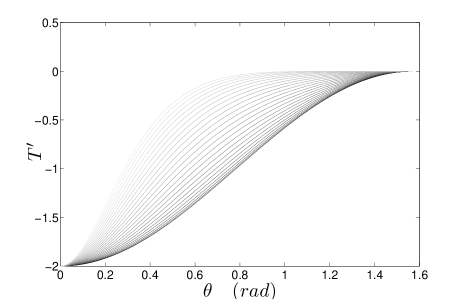
Figure 6: Plot of the trace $T^{\prime}=\mathrm{Tr}\{(\widehat{S}_{1}+\widehat{S}_{2}-\widehat{S}_{12})\rho_{3}\}$ versus $\theta$ (in radians) at different values of $k_{F}r$ for the 2-d configuration shown in Fig. 2. (Plot traces change from black to light gray as $k_{F}r$ is increased from 0.2 to 5.0 in steps of 0.2.)

A measure called negativity has been employed in Ref. Lunk in studying the entanglement properties of the NIFG. This quantity is defined for a trio of fermions $i,j,k$ as $N_{[i,jk]}=(||\rho_{3}^{T_{i}}||_{1}-1)/2$, where $||\rho_{3}^{T_{i}}||_{1}$ is the trace norm of the partial transpose of the three-fermion reduced density matrix $\rho_{3}$ of fermion $i$ with respect to fermions $j,k$. One of the advantages of working with EW operators rather than the negativity measure is in the identification of PPT entangled states. Using the condition (27) on the coefficients $a$, $b$, and $c$ in the NIFG expression for $\rho_{3}$ together with the entanglement witness ${}^{0}\mathcal{W}^{({\rm stab})}_{W}$, one can determine the configuration domain for which there exists PPT genuine $W$ entanglement with respect to the third fermion. The behavior of the trace $T^{\prime\prime}=\mathrm{Tr}\{^{0}\mathcal{W}^{({\rm stab})}_{W}\rho_{3}\}$ at three values of $k_{F}r$ is shown in Fig. 7 for both 1-d and 2-d configurations. Hence ${}^{0}\mathcal{W}^{({\rm stab})}_{W}$ is a partially non-decomposable $W$ EW for the third party since it can detect a PPT state with respect to the third fermion.

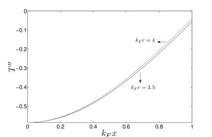
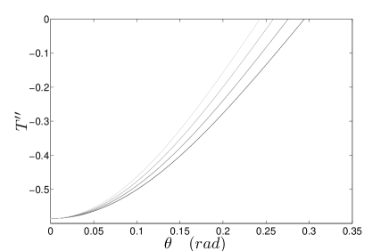
Figure 7: Trace $T^{\prime\prime}=\mathrm{Tr}\{^{0}\mathcal{W}^{({\rm stab})}_{W}\rho_{3}\}$ for detection of PPT genuine tripartite $W\setminus B$ entanglement with respect to the third particle. (a) The trace $T^{\prime\prime}$ is plotted versus $k_{F}x$ for the 1-d configuration shown in Fig. 1 at $k_{F}r=3.0$ and $k_{F}r=3.5$. (b) Trace $T^{\prime\prime}$ is plotted versus $\theta$ for the 2-d configuration shown in Fig. 2 for $3.0\leq k_{F}r\leq 4.0$ in steps of $0.25$. (Plot traces change from black to light gray as $k_{F}r$ is increased from 3.0 to 4.0.)

It is instructive to note that the eigenvectors corresponding to the eigenvalues of $\rho_{3}$ in (II) belong to the $W\setminus B$ class rather than $GHZ\setminus W$, affirming the absence of genuine $GHZ\setminus W$ entanglement in the NIFG. By way of proof, we first rewrite the three-body reduced density matrix in the standard form $\rho_{3}=\sum_{i}d_{i}|\alpha_{i}\rangle\langle\alpha_{i}|$, in which the $d_{i}$ are necessarily nonnegative. Then we assume there exists a $GHZ$ EW operator $\mathcal{W}_{GHZ}$ such that

$$\mathrm{Tr}(\mathcal{W}_{GHZ}\rho_{3})=\sum_{i}d_{i}\mathrm{Tr}(\mathcal{W}_{GHZ}|\alpha_{i}\rangle\langle\alpha_{i}|)$$ (80)

is negative. This assumption is contradictory if there is no $GHZ\setminus W$ contribution to the eigenvectors of $\rho_{3}$.

One question still remains (cf. Ref. Ved1, ): can there exist tripartite $W$-type entanglement in the NIFG, without any admixture biseparable or separable components, i.e., a state belonging purely to the $W\setminus B$ subset? This aspect can be investigated by establishing an upper bound on the trace of the product of a general density operator $\rho^{W}$ possessing $W\setminus B$ entanglement, and the three-fermion reduced density operator $\rho_{3}$. By virtue of Fermi exchange antisymmetry, it is sufficient to work with the operator

$$\varrho^{W}= |W_{1}\rangle\langle W_{1}|$$

$$= \frac{1}{3}(|001\rangle+|010\rangle+|100\rangle)(\langle 001|+\langle 010|+\langle 100|),$$ (81)

together with its transform

$$\varrho^{\prime W}=\left(\begin{array}[]{cc}\beta^{*}&\alpha\\ -\alpha^{*}&\beta\\ \end{array}\right)^{\otimes 3}\varrho^{W}\left(\begin{array}[]{cc}\beta&-\alpha\\ \alpha^{*}&\beta^{*}\\ \end{array}\right)^{\otimes 3}$$ (82)

under an arbitrary local unitary transformation, which again yields a purely $W$-type genuine entangled state. We have verified numerically that the value of $\mathrm{Tr}(\varrho^{\prime W}\rho_{3})$ is always less than one; hence the three-fermion reduced density operator of the NIFG cannot take the “pure” form $\varrho^{\prime W}$. This finding is confirmed for the explicit forms of $\rho(s,s^{\prime},s^{\prime\prime};t,t^{\prime},t^{\prime\prime})$ and $\rho_{3}$ given in Ref. Ved1, and reproduced in Eqs. (II) and (17). Consequently, one can conclude that in the NIFG, genuine tripartite entanglement only occurs in the three-fermion reduced density matrix $\rho_{3}$ in the company of 1-separable and/or 2-separable entanglement in other partitions: one cannot generate “pure” tripartite entanglement in the noninteracting Fermi gas.

V Conclusion

We have introduced new classes of entanglement witnesses (EWs) for the purpose of identifying genuine tripartite entanglement, i.e., $W\setminus B$ and $GHZ\setminus W$ states, in the three-fermion density matrix of the noninteracting Fermi gas (NIFG). We have reduced the task of constructing suitable EWs for this system to well-defined problems of linear programming. Considering EW operators inspired by a periodic spin chain model, EWs composed of the projection operators over the different classes of tripartite systems, and $GHZ$ stabilizer operators, we have found that the genuine tripartite entanglement present in the NIFG belongs to the $W\setminus B$ class. This result is confirmed in the structure of the eigenvectors of a general three-fermion reduced density matrix $\rho_{3}$ of the NIFG. We have seen that genuine tripartite entanglement does not occur in “pure” form, but instead it appears mixed with $B$ or $S$ components. Additionally, using a partially non-decomposable EW, we have been able to detect PPT genuine $W\setminus B$ entanglement with respect to the third party of a fermion trio in the NIFG. The general approach followed in this work can be applied to investigate multipartite entanglement in other quantum many-particle systems, whether consisting of fermions or bosons, possibly with higher spins, and whether the particles are interacting or noninteracting.

Acknowledgements

The authors thank D. Bruß and T. Vértesi for useful comments and M. A. Jafarizadeh, G. Najarbashi, and B. Dastmalchi for motivation and informative discussions. This research has been supported by the European Community Project N2T2. J.W.C. is grateful to the Johannes Kepler Universität Linz for fellowship support and the Institut für Theoretical Physik for hospitality during a sabbatical leave. He also thanks the Complexo Interdisciplinar of the University of Lisbon and the Department of Physics of the Technical University of Lisbon for their gracious hospitality, while acknowledging research support from Fundação para a Ciência e a Tecnologia of the Portuguese Ministério da Ciência, Tecnologia e Ensino Superior as well as Fundação Luso-Americana.

Appendix

To obtain the most general form for quantum states in the $W$ set, we consider the explicit form of $|\psi_{W}\rangle$ given in Eq. (23), together with an arbitrary local $SU(2)$ transformation applied for the different parties $i$ according to $|0\rangle_{i}\rightarrow\alpha_{i}|0\rangle_{i}+\beta_{i}|1\rangle_{i}$ and $|1\rangle_{i}\rightarrow\beta_{i}^{*}|0\rangle_{i}-\alpha_{i}^{*}|1\rangle_{i}$, with $|\alpha_{i}|^{2}+|\beta_{i}|^{2}=1$. We next write the general locally transformed $W$ vector as $|\Psi_{W}\rangle:=V|\psi_{W}\rangle$, where

$$V=\left(\begin{array}[]{cc}\beta_{1}^{*}&\alpha_{1}\\ -\alpha_{1}^{*}&\beta_{1}\\ \end{array}\right)\otimes\left(\begin{array}[]{cc}\beta_{2}^{*}&\alpha_{2}\\ -\alpha_{2}^{*}&\beta_{2}\\ \end{array}\right)\otimes\left(\begin{array}[]{cc}\beta_{3}^{*}&\alpha_{3}\\ -\alpha_{3}^{*}&\beta_{3}\\ \end{array}\right).$$ (A-1)

Rewriting the general $W$ vector as an expansion $|\Psi_{W}\rangle=\sum_{i,j,k=0,1}A_{ijk}|ijk\rangle$, the coefficients $A_{ijk}$ are determined as

$$A_{000}=\lambda_{0}\alpha_{1}\alpha_{2}\alpha_{3}+\lambda_{1}\beta_{1}^{*}\alpha_{2}\alpha_{3}+\lambda_{2}\beta_{1}^{*}\alpha_{2}\beta_{3}^{*}+\lambda_{3}\beta_{1}^{*}\beta_{2}^{*}\alpha_{3},$$

$$A_{001}=\lambda_{0}\alpha_{1}\alpha_{2}\beta_{3}+\lambda_{1}\beta_{1}^{*}\alpha_{2}\beta_{3}-\lambda_{2}\beta_{1}^{*}\alpha_{2}\alpha_{3}^{*}+\lambda_{3}\beta_{1}^{*}\beta_{2}^{*}\beta_{3},$$

$$A_{010}=\lambda_{0}\alpha_{1}\beta_{2}\alpha_{3}+\lambda_{1}\beta_{1}^{*}\beta_{2}\alpha_{3}+\lambda_{2}\beta_{1}^{*}\beta_{2}\beta_{3}^{*}-\lambda_{3}\beta_{1}^{*}\alpha_{2}^{*}\alpha_{3},$$

$$A_{011}=\lambda_{0}\alpha_{1}\beta_{2}\beta_{3}+\lambda_{1}\beta_{1}^{*}\beta_{2}\beta_{3}-\lambda_{2}\beta_{1}^{*}\beta_{2}\alpha_{3}^{*}-\lambda_{3}\beta_{1}^{*}\alpha_{2}^{*}\beta_{3},$$

$$A_{100}=\lambda_{0}\beta_{1}\alpha_{2}\alpha_{3}-\lambda_{1}\alpha_{1}^{*}\alpha_{2}\alpha_{3}-\lambda_{2}\alpha_{1}^{*}\alpha_{2}\beta_{3}^{*}-\lambda_{3}\alpha_{1}^{*}\beta_{2}^{*}\alpha_{3},$$

$$A_{101}=\lambda_{0}\beta_{1}\alpha_{2}\beta_{3}-\lambda_{1}\alpha_{1}^{*}\alpha_{2}\beta_{3}+\lambda_{2}\alpha_{1}^{*}\alpha_{2}\alpha_{3}^{*}-\lambda_{3}\alpha_{1}^{*}\beta_{2}^{*}\beta_{3},$$

$$A_{110}=\lambda_{0}\beta_{1}\beta_{2}\alpha_{3}-\lambda_{1}\alpha_{1}^{*}\beta_{2}\alpha_{3}-\lambda_{2}\alpha_{1}^{*}\beta_{2}\beta_{3}^{*}+\lambda_{3}\alpha_{1}^{*}\alpha_{2}^{*}\alpha_{3},$$

$$A_{111}=\lambda_{0}\beta_{1}\beta_{2}\beta_{3}-\lambda_{1}\alpha_{1}^{*}\beta_{2}\beta_{3}+\lambda_{2}\alpha_{1}^{*}\beta_{2}\alpha_{3}^{*}+\lambda_{3}\alpha_{1}^{*}\alpha_{2}^{*}\beta_{3}.$$

For the expectation values of the operators $\widehat{P}_{ij}$ of Eq. (IV.1) over the $W$ set, we now have

$$P^{W}_{12}:= \langle\Psi_{W}|\widehat{P}_{12}|\Psi_{W}\rangle$$

$$= |A_{000}|^{2}+|A_{001}|^{2}-|A_{010}|^{2}-|A_{011}|^{2}$$

$$-|A_{100}|^{2}-|A_{101}|^{2}+|A_{110}|^{2}+|A_{111}|^{2}$$

$$+(A_{010}A_{100}^{\ast}+A_{011}A_{101}^{\ast}+{\rm c.c}),$$

$$P^{W}_{23}:= \langle\Psi_{W}|\widehat{P}_{23}|\Psi_{W}\rangle$$

$$= |A_{000}|^{2}-|A_{001}|^{2}-|A_{010}|^{2}+|A_{011}|^{2}$$

$$+|A_{100}|^{2}-|A_{101}|^{2}-|A_{110}|^{2}+|A_{111}|^{2}$$

$$+(A_{001}A_{010}^{\ast}+A_{101}A_{110}^{\ast}+{\rm c.c.}),$$

$$P^{W}_{13}:= \langle\Psi_{W}|\widehat{P}_{13}|\Psi_{W}\rangle$$

$$= |A_{000}|^{2}-|A_{001}|^{2}+|A_{010}|^{2}-|A_{011}|^{2}$$

$$-|A_{100}|^{2}+|A_{101}|^{2}-|A_{110}|^{2}+|A_{111}|^{2}$$

$$+(A_{000}A_{101}^{\ast}+A_{001}A_{100}^{\ast}+A_{010}A_{111}^{\ast}+A_{011}A_{110}^{\ast}$$

$$+{\rm c.c.}),$$ (A-3)

while for the $W$-set expectation values of the stabilization operators $\widehat{S}_{i}$’s appearing in Eq. (63) we obtain

$$S^{W}_{1}:= (A_{000}A_{111}^{\ast}+A_{001}A_{110}^{\ast}+A_{010}A_{101}^{\ast}$$

$$+A_{011}A_{100}^{\ast}+{\rm c.c.}),$$

$$S^{W}_{2}:= |A_{000}|^{2}+|A_{001}|^{2}-|A_{010}|^{2}-|A_{011}|^{2}$$

$$-|A_{100}|^{2}-|A_{101}|^{2}+|A_{110}|^{2}+|A_{111}|^{2},$$

$$S^{W}_{1,2}:= (-A_{000}A_{110}^{\ast}-A_{001}A_{111}^{\ast}+A_{010}A_{100}^{\ast}$$

$$+A{011}A_{101}^{\ast}+A_{100}A_{010}^{\ast}+A_{101}A_{011}^{\ast}$$

$$-A_{110}A_{000}^{\ast}-A_{111}A_{001}^{\ast}+{\rm c.c.}).$$ (A-4)

Furthermore, for the operators $\widehat{P}_{i}$’s entering Eq. (24), the expectation values over the states of the $W$ class read

$$P^{W}_{1}= 2\langle\Psi_{W}|(|\Psi_{12}^{-}\rangle\langle\Psi_{12}^{-}|\otimes\textbf{I}+|\Psi_{13}^{-}\rangle\langle\Psi_{13}^{-}|\otimes\textbf{I}$$

$$+\textbf{I}\otimes|\Psi_{23}^{-}\rangle\langle\Psi_{23}^{-}|)|\Psi_{W}\rangle$$

$$= (A_{001}^{*}+A_{010}^{*}+A_{100}^{*})\times(A_{001}+A_{010}+A_{100}),$$

$$P^{W}_{2}= 3|\langle\Psi_{W}|W_{1}\rangle|^{2}$$

$$= (A_{001}^{*}+A_{010}^{*}+A_{100}^{*})\times(A_{001}+A_{010}+A_{100}),$$

$$P^{W}_{3}= 3|\langle\Psi_{W}|W_{2}\rangle|^{2}$$

$$= (A_{011}^{*}+A_{110}^{*}+A_{101}^{*})\times(A_{011}+A_{110}+A_{101}),$$

$$P^{W}_{4}= 2|\langle\Psi_{123}^{-}|\Psi_{W}\rangle|^{2}$$

$$= (A_{000}^{*}-A_{111}^{*})\times(A_{000}-A_{111}).$$ (A-5)

Similar relations are generated for the expectation values of the operators $P_{ij}^{B}$, $S^{B}_{i}$, and $P^{B}_{i}$.

To find a domain of the parameters in Eq. (35) such that $\mathcal{W}^{({\rm sp})}$ qualifies as a $W$ EW, we search for a convex polyhedron which is embedded in the domain spanned by the $P^{B}_{ij}$. To illustrate how the problem of finding a $W$ EW based on $\mathcal{W}^{(sp)}$ is reduced to the LP problem stated in (IV.1), one of the boundaries specified in Eq. (IV.1) for the convex polyhedron is determined as follows, the pattern for the others being similar Guh1 . With $|\psi_{B}\rangle=|\psi_{1}\rangle|\psi_{23}\rangle$ denoting an arbitrary biseparable state having entanglement among the second and third parties, we have

$$|-P^{B}_{12}-P^{B}_{13}+P^{B}_{23}|=$$

$$|\langle\psi_{B}|\sigma^{(1)}_{x}\sigma^{(2)}_{x}+\sigma^{(1)}_{y}\sigma^{(2)}_{y}+\sigma^{(1)}_{z}\sigma^{(2)}_{z}+\sigma^{(3)}_{x}+\sigma^{(3)}_{y}+\sigma^{(3)}_{z}$$

$$+\sigma^{(2)}_{x}\sigma^{(3)}_{x}+\sigma^{(2)}_{y}\sigma^{(3)}_{y}+\sigma^{(2)}_{z}\sigma^{(3)}_{z}|\psi_{B}\rangle|$$

$$\leq\;|\langle\psi_{B}|\sigma^{(2)}_{x}+\sigma^{(2)}_{y}+\sigma^{(2)}_{z}+\sigma^{(3)}_{x}+\sigma^{(3)}_{y}+\sigma^{(3)}_{z}|\psi_{B}\rangle|$$

$$+|\langle\psi_{B}|\sigma^{(2)}_{x}\sigma^{(3)}_{x}+\sigma^{(2)}_{y}\sigma^{(3)}_{y}+\sigma^{(2)}_{z}\sigma^{(3)}_{z}|\psi_{B}\rangle|$$

$$\leq\;1+\sqrt{8}.$$ (A-6)

The Schwartz inequality has been invoked in the second step. Parallel considerations apply in developing the other EWs introduced in this paper. In particular, for one of the boundaries associated with the stabilizer EW corresponding to Eq. (IV.3) we obtain

$$|-S^{B}_{1}+S^{B}_{2}-S^{B}_{12}|=$$

$$\;|\langle\psi_{B}|-\sigma^{(1)}_{x}\sigma^{(2)}_{x}\sigma^{(3)}_{x}+\sigma^{(1)}_{z}\sigma^{(2)}_{z}+\sigma^{(1)}_{y}\sigma^{(2)}_{y}\sigma^{(3)}_{x}|\psi_{B}\rangle|$$

$$\leq\;|\langle\psi_{B}|\sigma^{(2)}_{x}\sigma^{(3)}_{x}|\psi_{B}\rangle|+|\langle\psi_{B}|\sigma^{(2)}_{z}|\psi_{B}\rangle|$$

$$+|\langle\psi_{B}|\sigma^{(2)}_{y}\sigma^{(3)}_{x}|\psi_{B}\rangle|$$

$$\leq\;\sqrt{2}.$$ (A-7)

References

• (1) A. Osterloh, L. Amico, G. Falci, and R. Fazio, Nature 416, 608 (2002).
• (2) T. J. Osborne and M. A. Nielsen, Phys. Rev. A 66, 032110 (2002).
• (3) L. Amico, R. Fazio, A. Osterloh, and V. Vedral, Rev. Mod. Phys. 80, 517 (2007).
• (4) J. Schliemann, J. I. Cirac, M. Kus, M. Lewenstein, and D. Loss, Phys. Rev. A 64, 022303 (2001).
• (5) K. Eckert, J. Schliemann, D. Bruß, and M. Lewenstein, Annals of Phys. 299, 88-127 (2002).
• (6) G. Ghirardi, L. Marinatto, and T. Weber, J. Statistical Phys. 108, 49-122 (2002).
• (7) N. PaunkoviΔ‡, Y. Omar, S. Bose, and V. Vedral, Phys. Rev. Lett. 88, 187903 (2002).
• (8) P. Zanardi, Phys. Rev. A 65, 042101 (2002).
• (9) V. Vedral, Cent. Eur. J. Phys. 1, 2, 289-306 (2003).
• (10) S. Oh and J. Kim, Phys. Rev. A 69, 054305 (2004).
• (11) C. Lunkes, CΜ†. Brukner, and V. Vedral, Phys. Rev. Lett. 95, 030503 (2005).
• (12) M. R. Dowling, A. C. Doherty, and H. M. Wiseman, Phys. Rev. A 73, 052323 (2006).
• (13) T. VΓ©rtesi, Phys. Rev. A 75, 042330 (2007).
• (14) M. Lewenstein, B. Kraus, J. I. Cirac, and P. Horodecki, Phys. Rev. A 62, 052310 (2000).
• (15) A. AcΓ­n, D. Bruß, M. Lewenstein, and A. Sanpera, Phys. Rev. Lett. 87, 040401 (2001).
• (16) O. GΓΌhne, G. TΓ³th, and H. Briegel, New J. Phys. 7, 229 (2005).
• (17) D. Gottesman, Phys. Rev. A 54, 1862 (1996).
• (18) G. TΓ³th and O. GΓΌhne, Phys. Rev. Lett. 94, 060501 (2005).
• (19) G. TΓ³th and O. GΓΌhne, Phys. Rev. A 72, 022340 (2005).
• (20) W. Rudin, Functional Analysis (McGraw-Hill, New York, 1991).
• (21) M. A. Jafarizadeh, G. Najarbashi, and H. Habibian, Phys. Rev. A 75, 052326 (2007).
• (22) M. A. Jafarizadeh, G. Najarbashi, Y. Akbari, and H. Habibian, Eur. Phys. J. D 47, 233-255 (2008).