Exploring the photometric signatures of magnetospheres around Helium-strong stars

Abstract

The photometric variations due to magnetically confined material around He-strong stars are investigated within the framework of the Rigidly Rotating Magnetosphere (RRM) model. For dipole field topologies, the model is used to explore how the morphology of light curves evolves in response to changes to the observer inclination, magnetic obliquity, rotation rate and optical depth.

The general result is that double-minimum light curves arise when the obliquity and/or inclination are close to $90\degr$; no light variations are seen in the opposite limit; and for intermediate cases, single-minimum light curves occur. These findings are interpreted with the aid of a simple, analytical torus model, paving the way for the development of new photometric-based constraints on the fundamental parameters of He-strong stars. Illustrative applications to five stars in the class are presented.

1 Introduction

The Helium-strong stars are small class of chemically peculiar B stars, interpreted as an extension of the Ap/Bp phenomenon to higher effective temperatures (Osmer & Peterson, 1974). They are characterized by elevated and spatially inhomogeneous photospheric Helium abundances, and in most cases also exhibit strong magnetic fields (see Bohlender et al., 1987, and references therein). Spectroscopy of their time-varying Helium absorption lines often reveals that the surface abundance distribution is strongly correlated with field topology (Bohlender & Landstreet, 1988; Veto, 1990). These correlations lend support to models for the abundance anomalies that rely on the interplay between radiative and magnetic forces, either in the framework of elemental diffusion (e.g., Michaud, 1970), or in the context of wind mass loss (e.g., Hunger & Groote, 1999).

Of the He-strong stars exhibiting photometric variability (Pedersen & Thomsen, 1977), at least some can successfully be explained by invoking rotational modulation of the visible abundance inhomogeneities – so-called ‘spot’ models (see, e.g., Krtička et al., 2007). However, a different approach is required for other objects in the class, most notably the B2pe star $\sigma$ Ori E. The light curve of this star has a double-eclipse morphology (Hesser, Ugarte & Moreno, 1977), leading some authors (e.g., Hesser, Walborn & Ugarte, 1976) initially to suggest that the star is a mass-transfer binary. In fact, as further observational data have become available, an empirical picture for the star’s photometric and spectroscopic variability has emerged (Groote & Hunger, 1982), that augments a spot model with a pair of circumstellar clouds. These clouds absorb continuum photons as they transit the stellar disk, giving rise to the distinctive photometric minima; however, once off the disk they reveal themselves in H$\alpha$ line profiles as blue- and red-shifted emission components (e.g., Walborn & Hesser, 1976; Pedersen, 1979).

Recently, Townsend & Owocki (2005, hereafter TO-05) have developed a Rigidly Rotating Magnetosphere (RRM) model that provides the theoretical basis for this empirical picture. The model conjectures that plasma in the star’s radiatively driven wind, channeled by nearly rigid field lines, tends to accumulate at points where the effective (gravitational plus centrifugal) potential is at a local minimum. This steady accumulation leads to the development of a magnetosphere resembling a warped disk, which is supported by the centrifugal force and co-rotates rigidly with the star. For an oblique dipole field topology, the RRM model predicts that the magnetospheric density is highest in two regions – ‘clouds’ – situated along the twin intersections between the magnetic and rotational equators. In the specific case of $\sigma$ Ori E, the photometric and H$\alpha$ variations synthesized using the model show very good agreement with observations of the star (Townsend, Owocki & Groote, 2005).

In the present paper I apply the RRM model in a broader context, by exploring how the photometric signatures of magnetospheric plasma depend on fundamental parameters such as the observer inclination and magnetic obliquity (§2). The results from this parameter-space exploration are interpreted with the aid of a simple, analytic torus model (§3), and I discuss how they might be applied to constrain the parameters of He-strong stars (§4). The principal findings are then summarized (§5).

2 Exploration of parameter space

2.1 Light-curve synthesis

The RRM model as applied to a dipole magnetic topology is used to synthesize the light curves used for exploring parameter space. The same procedure described by Townsend et al. (2005, their §3.2) is followed; note therefore that the variability arising from abundance inhomogeneities is not considered. It is assumed that there is no decentering of the magnetic field, $\mathbf{a}=\mathbf{0}$ (eqn. 1, ibid.), and a canonical energy ratio parameter $\epsilon_{\ast}=10^{-3}$ (cf. TO-05, eqn. 38) is adopted throughout.

The remaining free parameters of the model are then the inclination $i$; the magnetic obliquity $\beta$; the ratio

$$\omega=\frac{\Omega}{\Omega_{\rm c}}$$ (1)

between the rotation frequency $\Omega$ and the critical frequency $\Omega_{\rm c}$; and an optical depth scale

$$\tau_{0}=\frac{\kappa\,\dot{M}\,t\,\omega^{4/3}}{R_{\ast}^{2}}.$$ (2)

This latter expression groups the opacity $\kappa$ (assumed constant) with various terms appearing in the RRM prescription for the density (TO-05, eqn. 35). The additional $\omega^{4/3}$ term comes from considering the rotational dependence of the total magnetospheric mass column between star and observer; its inclusion ensures that models having the same $\tau_{0}$ but differing $\omega$ exhibit approximately the same degree of light variations.

2.2 Varying $\beta$ and $i$

Figure 1: Light curves synthesized with varying inclination $i$ and obliquity $\beta$, in each case plotting the flux $F$ (in units of the unobscured stellar flux $F_{\ast}$) as a function of the rotation phase $\phi$; a rotation rate $\omega=0.5$ and an optical depth scale $\tau_{0}=10$ are assumed. The dotted horizontal lines indicate the level $F=F_{\ast}$.

To begin the exploration of parameter space, a grid of light curves is synthesized in $5\degr$ increments over the full intervals $0\degr\leq i\leq 90\degr$ and $0\degr\leq\beta\leq 90\degr$. In each case an intermediate rotation rate of $\omega=0.5$ is assumed, and an optical depth scale $\tau_{0}=10$ is chosen to produce variability on the $\sim 10\%$ level typical to He-strong stars. Figure 1 illustrates the resulting light curves, plotting the flux $F$ (in units of the unobscured stellar flux $F_{\ast}$) against the rotational phase $\phi$. For clarity only the curves at even multiples of $5\degr$ are shown, and the $i<30\degr$ cases are omitted because none exhibit any significant variability.

The figure clearly demonstrates how the character of the light curves is altered as $i$ and $\beta$ are changed. In the limit where either of these parameters is large, the curves exhibit a clear double-minimum (hereafter, ‘2-m’) morphology. In the opposite limit, and in particular for $i<30\degr$ as already mentioned, a non-varying, constant morphology (‘0-m’) is seen. For intermediate cases, falling approximately along a band extending from $\{i,\beta\}=\{30\degr,90\degr\}$ to $\{i,\beta\}=\{90\degr,0\degr\}$, a single light minimum (‘1-m’) occurs at phase $\phi=180\degr$.

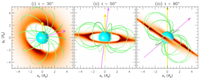
Figure 2: Maps of the column density $D$ in the observer’s image plane $(x_{\rm o},y_{\rm o})$, for three RRM configurations: (i) $\{i,\beta\}=\{30\degr,50\degr\}$ at a rotational phase $\phi=81\degr$, (ii) $\{i,\beta\}=\{50\degr,50\degr\}$ at $\phi=171\degr$, and (iii) $\{i,\beta\}=\{90\degr,50\degr\}$ at $\phi=81\degr$. (The phases are offset slightly from the ‘round-number’ values $90\degr$ and $180\degr$, to improve visual clues to the 3-D geometry). In all three cases, $\omega=0.5$. Black/opaque corresponds to highest column density, and white/transparent to lowest, with intermediate levels shown in orange. The central star is coloured blue, and the axes are drawn as arrows — yellow/upright for the rotation axis, and magenta/oblique for the magnetic axis. Moreover, selected field lines having a summit radius of $5\,R_{\rm p}$ (where $R_{\rm p}$ is the stellar radius at the rotational poles) are indicated in green.

To understand the origin of these three morphologies, Fig. 2 shows maps of the column density $D$ in the near-star regions of the circumstellar environment, for three configurations having $\beta=50\degr$ and $i=30\degr$, $50\degr$, and $90\degr$. The maps are calculated from an expression of the form

$$D(x_{\rm o},y_{\rm o})=\int\rho(x_{\rm o},y_{\rm o},z_{\rm o})\,\rm dz_{\rm o},$$ (3)

where $(x_{\rm o},y_{\rm o},z_{\rm o})$ are Cartesian coordinates in the observer’s reference frame, with $z_{\rm o}$ directed toward the observer, and $\rho$ is the local density predicted by the RRM model (cf. TO-05, eqn. 35). Panel (i) of the figure, plotting the $i=30\degr$ case, is typical of low-inclination systems. With the observer situated close to the rotation pole, the plasma trapped in the magnetosphere – lying in a disk between the rotational and magnetic equatorial planes – has no opportunity to pass between the observer and the star. Hence, an unvarying 0-m light curve is seen in these systems.

For panel (iii) the converse is true: with the observer in the rotational equatorial plane, the magnetospheric plasma transits the star twice per rotation cycle, and thus a 2-m light curve arises. In this particular case, symmetry requires that the minima occur at phases $\phi=90\degr$ and $270\degr$, with a half-cycle difference between them. However, as discussed in further detail below, a smaller phase difference $\Delta\phi$ is found for 2-m configurations having $i<90\degr$ and $\beta<90\degr$.

Panel (ii) illustrates the intermediate, $i=50\degr$ case, where the observer is not sufficiently close to the rotational equator for magnetospheric plasma to pass fully in front of the star. Instead, when the magnetic field is pointed away from the observer the plasma grazes the lower portions of the stellar limb, causing a 1-m light curve with the minimum centered at phase $\phi=180\degr$. This light curve is characterized by a reduced overall absorption, relative to the 2-m case shown in panel (iii).

As can be seen from the $\beta=50\degr$ row of light curves in Fig. 1, a smooth evolutionary sequence links the cases shown in panels (i), (ii) and (iii) of Fig. 2. As the observer moves from the rotational equator toward smaller $i$, the depth ($\equiv F_{\ast}-F$) at the twin light minima of the (initially, 2-m) light curve decreases; whereas, the depth at the intervening light maximum at $\phi=0.5$ increases. Eventually, these depth values cross over, with the result that the light curve transitions to a 1-m morphology. Following this switch-over (which in the $\beta=50\degr$ case occurs at $i\approx 60\degr$), the depth at the single remaining minimum at $\phi=180\degr$ declines toward lower $i$, and eventually vanishes in a further transition to a 0-m morphology.

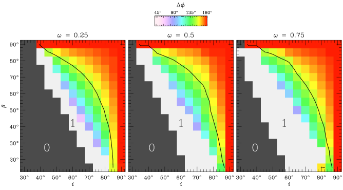
Figure 3: The phase difference $\Delta\phi$ between the minima in 2-m light curves, plotted in the $i$-$\beta$ plane for three differing rotation rates; in every case, $\tau_{0}=10$. The curve in each panel shows the contour $\Delta\phi=150\degr$, discussed in §4.2.2. Regions of the plane associated with 0-m and 1-m curves are shown in monochrome and labeled as ‘0’ and ‘1’, respectively.

The progressive distortion of light curves, as the 2-m to 1-m transition is approached, has an influence on the phase difference $\Delta\phi$ between the minima. To explore this influence, each light curve in the $i$-$\beta$ grid is analyzed using a simple algorithm that determines its morphology, and – if 2-m – measures the phase difference. The algorithm involves three steps:

1. If the total flux variation $\Delta F\equiv\max(F)-\min(F)$ is less than $0.01\,F_{\ast}$, then the light curve is classified as 0-m.

2. Otherwise, if the light curve exhibits two flux minima, and these minima are separated by flux maxima that both satisfy $F-\min(F)>0.15\Delta F$, then the light curve is classified as 2-m.

3. Otherwise, the light curve is classified as 1-m.

A minor complication arises when minima are cusped (see §2.3 and Fig. 4); then, the adopted phase of a minimum is determined by averaging the phases of the local minima on either side of the cusp.

Figure 3 plots the results of this analysis, showing the $\Delta\phi$ values for the 2-m light curves in the $i$-$\beta$ plane, and also indicating where in the plane 1-m and 0-m curves occur. (The middle panel of the figure shows the $\omega=0.5$ case considered in this section; the other two panels, corresponding to $\omega=0.25$ and $\omega=0.75$, are discussed in the following section). As before, the $i<30\degr$ region of the plane is uniformly 0-m and is therefore not shown; but in the present case, the $\beta<20\degr$ region is also omitted, because there the analysis algorithm gives unreliable results. This is more due to the difficulty in sensibly classifying the light curves in this region (in particular, see the $\{i,\beta\}=\{80\degr,10\degr\}$ and $\{90\degr,10\degr\}$ cases shown in Fig. 1), than to any particular limitation of the algorithm.

The figure confirms the previous finding that the 0-m and 2-m light curves are situated toward small and large angles, respectively, with the 1-m curves falling in between. However, it also reveals that $\Delta\phi$ depends quite regularly on $i$ and $\beta$. When either of these parameters is equal to $90\degr$, the phase difference is exactly one-half of a cycle; as already mentioned, this is required by symmetry. Away from these special cases, and toward the boundary between the 2-m and 1-m regions, $\Delta\phi$ is constant along contours running from low-$i$/high-$\beta$ corner down to the high-$i$/low-$\beta$ corner. The origin of this behaviour is explored further in §3.

2.3 Varying $\omega$

Figure 4: Light curves for a $\{i,\beta\}=\{70\degr,50\degr\}$ configuration, synthesized with $\tau_{0}=10$ and rotation rates $\omega=0.25$, 0.50, and 0.75. For clarity, the $\omega=0.50$ curve is displaced downward by $0.02\,F_{\ast}$, and the $\omega=0.75$ curve by $0.04\,F_{\ast}$.

The three panels of Fig. 3, showing the light-curve morphologies in the $i$-$\beta$ plane for $\omega=0.25$, 0.5, and 0.75, illustrate some of the effects of varying the rotation rate. The most obvious trend is the expansion of the 1-m region as $\omega$ is increased. This comes almost entirely at the expense of the 0-m region; almost no change is seen in the 2-m region, either in terms of its extent, or in terms of the $\Delta\phi$ values shown. Again, the reasons for such behaviour are explored further in §3.

Focusing now on an individual case, Fig. 4 plots the light curves for a $\{i,\beta\}=\{70\degr,50\degr\}$ configuration [chosen as half-way between the cases shown in panels (ii) and (iii) of Fig. 2], synthesized for the same three $\omega$ values above. As already noted for Fig. 3, the rotation rate has only a minor impact on the phase difference between the light minima; the measured differences are $\Delta\phi=118\degr$ for $\omega=0.25$, $\Delta\phi=116\degr$ for $\omega=0.50$, and $\Delta\phi=124\degr$ for $\omega=0.75$, amounting to only a $\sim 10\%$ variation from a factor-three increase in $\omega$.

However, a significant increase occurs in the width of the individual light minima toward more-rapid rotation. This indicates that the magnetospheric plasma is taking relatively longer to transit across the star, and follows from the approximate scaling of the RRM inner-edge radius with the Kepler radius,

$$R_{\rm K}=\frac{3\,R_{\rm p}}{2\,\omega^{2/3}}$$ (4)

(cf. TO-05, eqn. 12). As $\omega$ increases, both $R_{\rm K}$ and the inner edge moves in toward the star. Thus, the plasma takes a larger fraction of a rotation cycle to transit, and broader light minima ensue.

An additional effect of rapid rotation, seen in the $\omega=0.75$ panel of Fig. 4, is to produce cusping at the minima of the light curve. This effect, which is the characteristic hallmark of an optically thick yet geometrically thin disk, arises because the scale height $h_{\rm m}$ of the disk-like magnetosphere varies as $\sim R_{\rm K}^{3/2}\sim\omega^{-1}$ (cf. TO-05, eqn. 29).

2.4 Varying $\tau_{0}$

Figure 5: Light curves for a $\{i,\beta\}=\{70\degr,50\degr\}$ configuration, synthesized for $\omega=0.50$ and optical depth scales $\tau_{0}=5$, 10, and 15. For clarity, the $\tau_{0}=10$ curve is displaced downward by $0.02\,F_{\ast}$, and the $\tau_{0}=15$ curve by $0.04\,F_{\ast}$.

For the sake of completeness Fig. 5 plots the light curves for the same $\{i,\beta\}=\{70\degr,50\degr\}$ configuration considered previously, but synthesized this time with a fixed rotation rate $\omega=0.50$ and varying optical depth scale: $\tau_{0}=5$, 10 and 15. The maximum depths of the light curves – $0.037\,F_{\ast}$, $0.069\,F_{\ast}$ and $0.099\,F_{\ast}$, respectively – increase approximately linearly with $\tau_{0}$. This result is a natural consequence of the fact that the magnetospheric densities (cf. TO-05, eqn. 35) are proportional to $\tau_{0}$. As in the preceding section, however, the change in phase difference is small: in the direction of increasing $\tau_{0}$, $\Delta\phi=120\degr$, $116\degr$ and $114\degr$.

3 A torus model

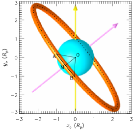
Figure 6: The torus model for a $\{i,\upsilon_{\rm t},R_{\rm t}\}=\{70\degr,50\degr,3.5\,R_{\rm p}\}$ configuration, seen at rotational phase $\phi=92\degr$; the torus is colored orange, while the star and axes are as in Fig. 2. The dotted line shows the ellipse corresponding to the sky projection of the torus; this ellipse is centered at point O, and intersects the stellar limb at points A and B. The arc AB has length $\ell$, and the line OM – where M is the midpoint of the arc – is the semi-minor axis $b$ of the ellipse.

The previous sections explore how RRM light-curve morphology is sensitive to parameters such as $i$, $\beta$, and $\omega$. A number of interesting dependencies emerge, as seen for instance in Fig. 3. To gain a measure of insight into these dependencies, the present section introduces an idealized, analytic torus model for the formation of the light curves.

In this model, flux variations arise due to obscuration of a spherical star by an optically thick, oblique, co-rotating torus of circumstellar material. Assuming that the torus is narrow compared to the stellar radius, the observed flux at any instant can be approximated by considering the fraction of the stellar disk obscured:

$$F=F_{\ast}\left(1-\frac{\ell d_{\rm t}}{\pi R_{\ast}^{2}}\right).$$ (5)

Here, $R_{\ast}$ is the stellar radius, $d_{\rm t}$ ($\ll R_{\ast}$) is the torus cross-sectional diameter, and $\ell$ is the length of the torus arc (if any) covering the stellar disk. For $R_{\rm t}$ not too close to the stellar radius $R_{\ast}$, this arc length is approximated by

$$\ell\approx 2\sqrt{\max(R_{\ast}^{2}-b^{2},0)},$$ (6)

where $b$ is the semi-major axis of the ellipse that is the projection of the torus on the plane of the sky (see Fig. 6). If the torus plane is tilted by an angle $\upsilon_{\rm t}$ to the rotation axis, it can be shown that

$$b=R_{\rm t}|\cos i\cos\upsilon_{\rm t}+\sin i\sin\upsilon_{\rm t}\cos\phi|,$$ (7)

where $R_{\rm t}$ is the radius of the torus.

Even before light curves are synthesized, these expressions can be used to demonstrate that the torus model reproduces the same three light-curve morphologies found previously. For any light variations whatsoever to occur, $b$ must be smaller than $R_{\ast}$ at some point during the rotation cycle. Assuming that $0\degr\leq i\leq 90\degr$ and $0\degr\leq\upsilon_{\rm t}\leq 90\degr$, this is is equivalent to the requirement

$$\cos(i+\upsilon_{\rm t})<\frac{R_{\ast}}{R_{\rm t}}.$$ (8)

If this condition is fulfilled, then the light curve exhibits a single or double minimum morphology depending on whether the torus passes across the centre of the stellar disk:

$$\cos(i+\upsilon_{\rm t})\begin{cases}>0&\qquad\mbox{1-m}\\ <0&\qquad\mbox{2-m}\end{cases}$$ (9)

In the 1-m case, the flux minimum always occurs at phase $\phi=180\degr$. In the 2-m case, the minima arise when

$$\cos i\cos\upsilon_{\rm t}=-\sin i\sin\upsilon_{\rm t}\cos\phi,$$ (10)

so that the phase difference is given by

$$\Delta\phi=2\cos^{-1}(\cot i\cot\upsilon_{\rm t})$$ (11)

A similar expression has been derived by Shore & Brown (1990, their eqn. 2), but in their case $\beta$ appears in the place of $\upsilon_{\rm t}$.

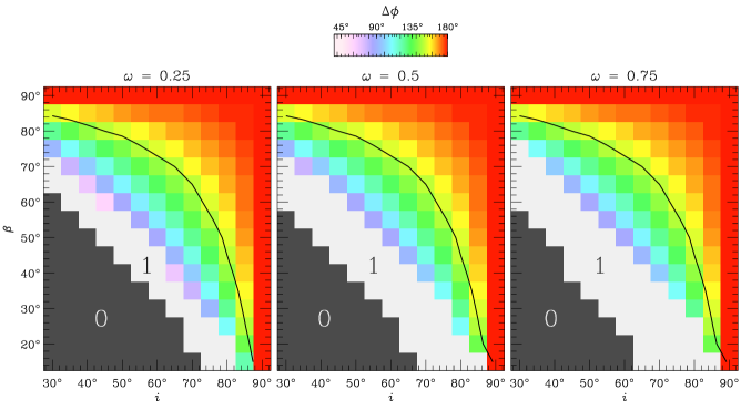
Figure 7: As for Fig. 3, except that the light curves are calculated using the torus model rather than the RRM model; in every case, $d_{\rm t}=0.1\,R_{\ast}$.

To now relate the foregoing analysis back to the RRM model, representative values are chosen for the torus radius $R_{\rm t}$ and tilt angle $\upsilon_{\rm t}$. For the former, the Kepler radius $R_{\rm K}$ (cf. eqn. 4) is the appropriate choice; for the latter, Appendix (A) argues that

$$\upsilon=\beta-\tan^{-1}\left(\frac{\sin 2\beta}{5+\cos 2\beta}\right)$$ (12)

furnishes a good characterization of the mean tilt of the magnetospheric disk. Adopting these values, and further assuming a diameter $d_{\rm t}=0.1R_{\ast}$, eqns. (5–7) are used to synthesized a $\beta-i-\omega$ grid of light curves. These data are analyzed using the algorithm described in §2.2, and Fig. 7 plots the results in the same format as Fig. 3.

The two figures shown a good measure of qualitative agreement. Specific characteristics of the RRM model that are correctly reproduced by the torus model include:

• the three differing light-curve morphologies (0-m, 1-m and 2-m), and their general locations in the $\{i,\beta\}$ plane;

• the fact that the phase differences of 2-m light curves are insensitive to rotation rate; this follows from eqn. (11), which has no dependence (explicit or implicit) on $\omega$;

• likewise, the fact that the boundary between the 1-m and 2-m regions is insensitive to the rotation rate; this follows from eqn. (9), which again has no dependence on $\omega$;

• conversely, the fact that the boundary between the 0-m and 1-m regions does depend on the rotation rate, moving toward lower $i$ as $\omega$ is increased; this is due to the identification $R_{\rm t}=R_{\rm K}$, which introduces an implicit dependence on $\omega$ into eqn. (8);

• finally, although not shown in the figures, the increase in the width of 2-m light minima toward more-rapid rotation.

At a quantitative level, the agreement between the two models is more limited; for instance, at large $\beta$ the torus model predicts an extension of the 2-m region to low inclinations, which is not seen in the RRM model. [In this particular case, the discrepancy arises because high-$\beta$ magnetospheres are punctured by cone-shape voids over the rotational poles (see TO-05, fig. 3), and therefore do not produce light variations when viewed from low inclinations.] Such discrepancies mean that the torus model should not be used as the sole basis for data analysis. However, the bulleted list above is ample proof that – as a tool for data interpretation – the model has many useful insights to offer.

4 Discussion

4.1 Photometric diagnostics

The preceding sections demonstrate that the light variations arising from a RRM depend on fundamental stellar parameters in a way that is simple, regular and straightforward to understand. Given these qualities, it is reasonable to conjecture that observations of these variations, in He-strong stars and similar objects, could be used in tandem with other diagnostics such as magnetic field measurements to establish constraints on the parameters of these stars.

The success of this endeavour rests to a large part on the validity of the RRM model, since it is from diagrams such as Fig. 3 – constructed with the aid of the model – that reliable diagnostics are developed. In this respect, the close correspondence between the observed and synthesized H$\alpha$ variations of $\sigma$ Ori E (Townsend et al., 2005) has lent considerable empirical support to the model. Moreover, recent rigid-field hydrodynamical simulations by Townsend, Owocki & ud-Doula (2007), and magnetohydrodynamical simulations by ud-Doula, Owocki & Townsend (2007), have provided confirmation of the theoretical underpinnings of the model.

Of equal importance, however, is the problem of disentangling the light variations arising from photospheric abundance inhomogeneities on the one hand, and from magnetospheric plasma on the other. For certain configurations, these two mechanisms can produce variability that appears ostensibly the same. For instance, the $\{i,\beta\}=\{70\degr,20\degr\}$ magnetospheric light curve in Fig. 1, showing a single, broad minimum, might easily be confused with the rotational modulation arising from a spot-like photospheric inhomogeneity. In situations like these, other diagnostics such as spectroscopy or polarimetry must be used to lift the degeneracy and correctly identify which mechanism is responsible for the observed variability.

In the majority of cases, however, the morphologies of the light curves produced by the alternative mechanisms are rather different. Especially toward large $i$ and/or $\beta$, the light variations caused by magnetospheric plasma tend to be much more rapid (relative to the rotation period) than could plausibly be achieved by photospheric inhomogeneities. Thus, as a simple rule, faster variations can be attributed to the magnetosphere, and slower variations to the photosphere. By way of illustration, the following section applies this heuristic to five He-strong stars, in some cases examining whether the constraints provided by Fig. 3 are consistent with literature values for these stars’ parameters, and in other cases using such constraints to make predictions.

4.2 Application to He-strong stars

4.2.1 HD 37017

The light variations of this star (e.g., Bolton et al., 1998) show a smooth, sinusoidal character, favouring a photospheric rather than magnetospheric origin. Bohlender et al. (1987) derive $42\degr\lesssim\beta\lesssim 59\degr$ and $23\degr\lesssim i\lesssim 37\degr$ from magnetic and period measurements; with reference to Fig. 3, these values mostly fall in the 0-m region and are therefore consistent with the apparent lack of a magnetospheric signature.

4.2.2 HD 37479 ($\sigma$ Ori E)

As already discussed in §1, this star exhibits distinctive 2-m light variations that are consistent with a magnetospheric origin. That said, certain aspects of its light curve, such as the unequal depths of the minima and the ‘emission’ feature after the secondary minimum, appear more likely be of photospheric origin (see Townsend et al., 2005; note that these authors explained the depth asymmetry by instead invoking a decentered dipole).

Nevertheless, this photospheric signal is unlikely to have much effect on the measured phase difference $\Delta\phi\approx 150\degr$ between the two minima. This value is indicated in each panel of Fig. 3 by the contour curves. Along these contours the combined angle $\beta+i$ varies between $\sim 105\degr$ and $\sim 135\degr$, which led Townsend et al. (2005) to adopt the approximate relation $\beta+i\approx 130\degr$ in developing their model for the star. This constraint is consistent with the parameters $\{i,\beta\}\approx\{70\degr,56\degr\}$ derived by Shore & Brown (1990) from consideration of magnetic and IUE data.

4.2.3 HD 37776

This star has a rather non-sinusoidal light curve, with a single, very broad minimum suggestive of a photospheric origin. Detailed modeling by Krtička et al. (2007) demonstrates that, indeed, the photospheric abundance distribution determined spectroscopically by Khokhlova et al. (2000) can also faithfully reproduce the star’s light curve. Note that the star has a quadrapolar field topology (Thompson & Landstreet, 1985); although the RRM model can in principle be applied to any arbitrary field topology, studies so far (including the present paper) focus on the simplest and commonest case of a dipole field. Thus, the absence of a clear magnetospheric signature in the light curve of HD 37776 cannot, without further modeling, be used to constrain $i$ or $\beta$.

4.2.4 HD 64740

This star is the brightest in the He-strong class, yet it exhibits almost no photometric variations (Pedersen & Thomsen, 1977). Bohlender et al. (1987) derive $\beta\lesssim 76\degr$ and $i\gtrsim 41\degr$ from magnetic and period measurements. Given the absence of any variability, the boundary between the 0-m and 1-m regions in Fig. 3 (assuming $\omega=0.5$) can be used to further constrain the parameters as $\beta+2i\lesssim 150\degr$.

4.2.5 HD 182180

This star has recently been shown to be He-strong, and to exhibit H$\alpha$ and photometric variations, by Rivinius et al. (2007). Observational data remain scarce, but the 2-m, $\Delta\phi=180\degr$ morphology of the double-wave light curve is consistent with $\beta=90\degr$ and/or $i=90\degr$. The light minima are rather too broad to convincingly rule out a photospheric origin, but given the star’s extreme rotation period of $0.521\,{\rm d}$, the widths of the minima are wholly consistent with a near-critical, $\omega\approx 1$ configuration.

5 Summary

The RRM model has been used to explore how the light variations due to magnetospheric plasma depend on the parameters $\beta$, $i$, $\omega$, and $\tau_{0}$ (§2). Double-minimum morphologies are found toward large values of the inclination $i$ and/or obliquity $\beta$; single-minimum and non-varying morphologies occur for progressively smaller values of these parameters. In the double-minimum cases, the phase difference $\Delta\phi$ between the minima depends primarily on $i$ and $\beta$, with almost no sensitivity to the rotation rate $\omega$ or optical depth scale $\tau_{0}$.

Insight into these findings has been developed with the aid of an analytic torus model (§3). Although not in complete quantitative agreement with the RRM model, the torus model is able to explain all of the qualitative results from the parameter-space exploration. Applying these results, constraints on the obliquity and inclination of four He-strong stars are derived from their light curves (§4); these are found to be generally consistent with values quoted in the literature.

Appendix A The disk tilt angle

As discussed in §1, the RRM model predicts magnetospheres that resemble a warped disk. A characteristic disk tilt angle $\upsilon$ with respect to the rotation axis can be obtained by considering the locus formed by the minima of the dimensionless effective potential,

$$\Psi=-\frac{1}{\gamma\sin^{2}\tilde{\theta}}-\frac{\gamma^{2}\sin^{4}\tilde{\theta}}{2}\left[\sin^{2}\tilde{\theta}\,\sin^{2}\tilde{\phi}+\mbox{}\phantom{\left(\sin\beta\,\cos\tilde{\theta}+\cos\beta\,\sin\tilde{\theta}\,\cos\tilde{\phi}\right)^{2}}\right.\\ \left.\left(\sin\beta\,\cos\tilde{\theta}+\cos\beta\,\sin\tilde{\theta}\,\cos\tilde{\phi}\right)^{2}\right]$$ (13)

(cf. TO-05, eqn. 22). Here, $\tilde{\theta}$ is the magnetic colatitude on the dipole field line having summit radius $\gamma$ (in units of the Kepler radius $R_{\rm K}$; cf. eqn. 4) and magnetic azimuth $\tilde{\phi}$. The conditions for a potential minimum are that

$$\frac{\partial\Psi}{\partial\tilde{\theta}}=0,\qquad\frac{\partial^{2}\Psi}{\partial\tilde{\theta}^{2}}>0.$$ (14)

As discussed by TO-05, algebraic solution of these equations for general $\beta$, $\gamma$, and $\tilde{\phi}$ is not possible. However, the $\tilde{\phi}=90\degr,270\degr$ meridional planes are exceptions – for these, it is straightforward to demonstrate that minima occur at the magnetic equator, $\tilde{\theta}=90\degr$.

Immediately adjacent to these special cases, for instance in the $\tilde{\phi}=90\degr+\tilde{\delta}_{\phi}$ meridional plane for $|\tilde{\delta}_{\phi}|\ll 1$, the continuity of the disk requires that the potential minimum should be at $\tilde{\theta}=90\degr+\tilde{\delta}_{\theta}$, where $|\tilde{\delta}_{\theta}|\ll 1$ also. Substituting this trial solution into the zero-gradient condition in (14), and neglecting terms of quadratic- or higher-order in $\tilde{\delta}_{\phi}$ and $\tilde{\delta}_{\theta}$, leads to the equation

$$-\frac{\gamma^{2}\sin 2\beta}{2}\,\tilde{\delta}_{\phi}+\left[-\frac{2}{\gamma}+\frac{\gamma^{2}(5+\cos 2\beta)}{2}\right]\,\tilde{\delta}_{\theta}=0.$$ (15)

For field lines extending far outside the Kepler radius (i.e., $\gamma\gg 1$), the solution is then found as

$$\tilde{\delta}_{\theta}=\frac{\sin 2\beta}{5+\cos 2\beta}\,\tilde{\delta}_{\phi}.$$ (16)

The local tilt angle $\tilde{\upsilon}$ of the disk with respect to the magnetic axis is determined from

$$\tan\tilde{\upsilon}=-\frac{\tilde{\delta}_{\theta}}{\tilde{\delta}_{\phi}}=-\frac{\sin 2\beta}{5+\cos 2\beta}.$$ (17)

Thus, the tilt angle with respect to the rotational axis follows as

$$\upsilon=\beta+\tilde{\upsilon}=\beta-\tan^{-1}\left(\frac{\sin 2\beta}{5+\cos 2\beta}\right).$$ (18)

Strictly speaking, this value cannot be applied across the whole of an RRM disk, due to the warping that arises when $\beta>0\degr$. However, as can be seen from Fig. 3 of TO-05, the disk tilt in the $\tilde{\phi}=90\degr,270\degr$ meridional planes furnishes a good approximation to the mean disk tilt, and therefore is well suited to characterizing the overall disk orientation.

References

- Bohlender & Landstreet (1988) Bohlender D. A., Landstreet J. D., 1988, in Cayrel de Strobel G., Spite M., eds, Proc. IAU Symp. 132: The Impact of Very High S/N Spectroscopy on Stellar Physics. p. 309
- Bohlender et al. (1987) Bohlender D. A., Landstreet J. D., Brown D. N., Thompson I. B., 1987, ApJ, 323, 325
- Bolton et al. (1998) Bolton C. T., Harmanec P., Lyons R. W., Odell A. P., Pyper D. M., 1998, A&A, 337, 183
- Groote & Hunger (1982) Groote D., Hunger K., 1982, A&A, 116, 64
- Hesser et al. (1977) Hesser J. E., Ugarte P. P., Moreno H., 1977, ApJ, 216, L31
- Hesser et al. (1976) Hesser J. E., Walborn N. R., Ugarte P. P., 1976, Nature, 262, 116
- Hunger & Groote (1999) Hunger K., Groote D., 1999, A&A, 351, 554
- Khokhlova et al. (2000) Khokhlova V. L., Vasilchenko D. V., Stepanov V. V., Romanyuk I. I., 2000, Astronomy Letters, 26, 177
- Krtička et al. (2007) Krtička J., Mikuláček Z., Zverko J., Žižńovský J., 2007, A&A, 470, 1089
- Michaud (1970) Michaud G., 1970, ApJ, 160, 641
- Osmer & Peterson (1974) Osmer P. S., Peterson D. M., 1974, ApJ, 187, 117
- Pedersen (1979) Pedersen H., 1979, A&AS, 35, 313
- Pedersen & Thomsen (1977) Pedersen H., Thomsen B., 1977, A&AS, 30, 11
- Rivinius et al. (2007) Rivinius T., Štefl S., Townsend R. H. D., Baade D., 2007, A&A, submitted
- Shore & Brown (1990) Shore S. N., Brown D. N., 1990, ApJ, 365, 665
- Thompson & Landstreet (1985) Thompson I. B., Landstreet J. D., 1985, ApJ, 289, L9
- Townsend & Owocki (2005) Townsend R. H. D., Owocki S. P., 2005, MNRAS, 357, 251
- Townsend et al. (2005) Townsend R. H. D., Owocki S. P., Groote D., 2005, ApJ, 630, L81
- Townsend et al. (2007) Townsend R. H. D., Owocki S. P., ud-Doula A., 2007, MNRAS, submitted
- ud-Doula et al. (2007) ud-Doula A., Owocki S. P., Townsend R. H. D., 2007, MNRAS, in preparation
- Veto (1990) Veto B., 1990, Ap&SS, 174, 111
- Walborn & Hesser (1976) Walborn N. R., Hesser J. E., 1976, ApJ, 205, L87