Abstract

We propose a measurement on the elastic $\pi\pi$ scattering phase shift difference $\delta^{0}_{0}-\delta^{2}_{0}$ through $\Psi^{\prime}\rightarrow J/\Psi\,\pi^{+}\pi^{-}$ process in future high statistics BES-III experiment. The decay amplitude is constructed with seven Lorentz invariant form-factors and is compared with their theoretical estimation. It is found that the phase shift difference can be obtained, based on a Monte Carlo study and it is expected the phase shift in the energy region between 350 MeV to 550 MeV can be measured at future BES-III.

Key words: phase shift; $\pi\pi$ scattering; $\Psi^{\prime}$ decays.
PACS: 11.80.Et; 13.20.Gd; 13.75.Lb.

1 Introduction

In recent years, the operation of a number of high precision, high statistics experimental machines, varying from fixed target experiments to $B$ factories, opens a new era for precision hadronic experiments. Based on that, both experimental and theoretical studies on low energy $\pi\pi$ and $\pi K$ system produced in production processes have also received revived interests. The importance of these studies follows from the fact that when final state theorem applies, one can extract low energy elastic scattering phase shifts in the related channels through a partial wave analysis. The information on $\pi\pi$, $\pi K$ phase shifts then provides a crucial ingredient in understanding the dynamics of goldstone bosons and the spontaneous breaking of chiral symmetry.

The experimental and theoretical activities in the last few years mainly focused on semi-leptonic and hadronic $D$ decays (see for example, Refs. [1] – [4]). It is known that in $D$ semi-leptonic decays $p$–wave dominates, and the more interesting $s$–wave component is small. In this paper we re-investigate the $\pi\pi$ final state interactions in the $\Psi^{\prime}\rightarrow J/\Psi\pi^{+}\pi^{-}$ process. Here $s$–wave dominates and the next contribution comes from the tiny $d$–wave. The existence of the latter is however crucial for exploring the $s$–wave phase motion through interference effect. The decay product under concern is a three body final state, the $J/\Psi$ particle is however irrelevant to any final state interactions here. Using color transparency argument it is understood that the effect from rescattering between the $J/\Psi$ and one of the pions is negligible. Another important fact is that, in the kinematic region under concern, between the initial $\Psi^{\prime}$ and the final $J/\Psi\pi\pi$ there is no other on-shell intermediate hadronic state available (or are double OZI suppressed and hence negligible). Hence the final state theorem is applicable to the $\pi\pi$ system in $\Psi^{\prime}\rightarrow J/\Psi\pi^{+}\pi^{-}$ process.

The $\Psi^{\prime}\rightarrow J/\Psi\pi^{+}\pi^{-}$ process has been the subject of a number of previous publications ([5]– [7]). In Ref. [8], the author proposed a method to extract $\pi\pi$ phase shift from $\Psi^{\prime}\rightarrow J/\Psi\pi^{+}\pi^{-}$, similar to Pais-Treiman [9] method for obtaining $\pi\pi$ phase shifts from $K_{l4}$ decays, but only considered three partial wave amplitudes for reducing the difficulty of the analysis. A similar method [10] was also proposed in $\Upsilon(3S)\to\Upsilon(1S)\pi\pi$ process but only the lowest order in the pion momentum expansion was considered. In this work we are able to provide a more general parametrization to the decay amplitude comparing with what is given in most of previous papers. Our parametrization will be discussed in section 2. Furthermore we will also provide a Monte Carlo study in section 3 to test the stability and reliability to use our parametrization to extract the phase shift data.

2 General structure of the $\Psi^{\prime}\rightarrow J/\Psi\,\pi^{+}\pi^{-}$ decay amplitude

2.1 The Lorentz invariant form-factors

There are 3 independent momenta $p_{\pi^{+}},p_{\pi^{-}},p_{J/\Psi}=p_{3}$, which can be re-expressed in 3 variables $q=p_{\pi^{+}}+p_{\pi^{-}},p=p_{\pi^{+}}-p_{\pi^{-}},$ and $p_{3}$. The three independent momenta can form 2 independent Lorentz invariant products, chosen as $q^{2}$ and $p\cdot p_{3}$ here. Then,

$$q^{2}=s,$$ (1)

$$p^{2}=-s\rho^{2}=4m_{\pi}^{2}-s,$$ (2)

$$p_{3}^{2}=M_{\Psi}^{2},$$ (3)

$$q\cdot p=0,$$ (4)

$$q\cdot p_{3}=\frac{1}{2}(M_{\Psi^{\prime}}^{2}-M_{\Psi}^{2}-s),$$ (5)

with the kinematics factor of dipion system $\rho=\sqrt{1-{4m_{\pi}^{2}\over s}}$, the energy and the momenta of $J/\Psi$ in the lab frame (the $\Psi^{\prime}$ rest frame), which $E_{3}=(M_{\Psi^{\prime}}^{2}+M_{\Psi}^{2}-s)/(2M_{\Psi^{\prime}})$ and $|\vec{p}_{3}|=\sqrt{E_{3}^{2}-M_{\Psi}^{2}}$ are functions of $q^{2}$. Moreover, $p\cdot p_{3}$ can be expressed in the $\Psi^{\prime}$ rest frame with the variables in the dipion rest frame,

$$p\cdot p_{3}=2\gamma|\vec{p}_{\pi\pi}^{\,\,*}|\cos\theta_{\pi}^{*}(\beta E_{3}+|\vec{p}_{3}|),$$ (6)

where $|\vec{p}_{\pi\pi}^{\,\,*}|=\rho\sqrt{s}/2$ is the three momenta of $\pi$ in the dipion rest frame and $\theta_{\pi}^{*}$ is the angle between the direction of $\pi^{+}$ and direction opposite to the final $J/\Psi$ in the dipion rest frame, see Fig. 1 for illustration. $\beta=\sqrt{1-\frac{1}{\gamma^{2}}}$ is the boost factor from the dipion rest frame to the lab frame with $\gamma=(M_{\Psi^{\prime}}^{2}-M_{\Psi}^{2}+s)/(2M_{\Psi^{\prime}}\sqrt{s})$.

Figure 1: $\theta_{3}$ is the angle between the beam and $J/\Psi$ in the $\Psi^{\prime}$ rest frame. $\theta_{\pi}^{*}$ is the angle between the $J/\Psi$ direction and the $\pi^{+}$ in the di-pion rest frame, $\phi$ is the azimuthal angle between the beam $J/\Psi$ plane and $\pi^{+}\pi^{-}$ plane in the $\Psi^{\prime}$ rest frame (not drawn in the figure).

Denoting the polarization vector of $\Psi^{\prime}$ and $J/\Psi$ by $\epsilon^{\prime}$ and $\epsilon$ respectively, we can form five invariants bilinear in $\epsilon^{\prime}\epsilon^{*}$:

$$(\epsilon\cdot\epsilon^{\prime}),\,\,\,(\epsilon\cdot q)(\epsilon^{\prime}\cdot q),\,\,\,(\epsilon\cdot p)(\epsilon^{\prime}\cdot p),\,\,\,(\epsilon\cdot q)(\epsilon^{\prime}\cdot p),\,\,\,(\epsilon\cdot p)(\epsilon^{\prime}\cdot q).$$

Hence, the amplitude have the independent structure:

$$T=(\epsilon\cdot\epsilon^{\prime})F_{0}+(\epsilon\cdot q)(\epsilon^{\prime}\cdot q)F_{1}+(\epsilon\cdot p)(\epsilon^{\prime}\cdot p)F_{2}+(\epsilon\cdot q)(\epsilon^{\prime}\cdot p)F_{3}+(\epsilon\cdot p)(\epsilon^{\prime}\cdot q)F_{4}.$$ (7)

$F_{i}$ are the functions of $s$ and $p\cdot p_{3}$ and these allow us to do partial wave decomposition according to $\theta_{\pi}^{*}$.

2.2 Partial wave decomposition

From Ref. [11], we obtain the basis of tensors

$$\tilde{t}^{(0)}=1,$$ (8)

$$\tilde{t}^{(1)}=p^{\mu},$$ (9)

$$\tilde{t}^{(2)}=p^{\mu}p^{\nu}-\frac{1}{3}p^{2}\tilde{g}^{\mu\nu},\,\,\,\,\hbox{with}\,\,\,\tilde{g}^{\mu\nu}=g^{\mu\nu}-\frac{q^{\mu}q^{\nu}}{q^{2}},$$ (10)

where every tensor $\tilde{t}^{(L)}$ transforms irreducibly as a tensor of spin $L$. In the present problem we have the four vectors, $q^{\mu}$, $p_{3}^{\mu}$, $\epsilon^{\prime\mu}$ and $\epsilon^{\mu}$ ,which are independent on $\theta_{\pi}^{*}$. We can build the independent Lorentz scalars:

$$q^{2},\,\,\,q\cdot\epsilon,\,\,\,q\cdot\epsilon^{\prime}\,\,\,\,\hbox{and}\,\,\,\,\epsilon\cdot\epsilon^{\prime}.$$

The available Lorentz vectors would be

$$q^{\mu},\,\,\,p_{3}^{\mu},\,\,\,\epsilon^{\prime\mu},\,\,\,\epsilon^{\mu}.$$

With these we go first to build $L=0$ quantities. This can only be obtained through $\tilde{t}^{(0)}$ and taking into account that the polarization vectors $\epsilon^{\prime}$ and $\epsilon$ must always be contracted at the end,

$$S=\tilde{t}^{(0)}\cdot\{I^{(0)}_{1}(s)(\epsilon^{\prime}\cdot\epsilon)+I^{(0)}_{2}(s)(\epsilon^{\prime}\cdot q)(\epsilon\cdot q)\},$$ (11)

which can be expressed through $S=\epsilon^{\prime\mu}\epsilon^{\nu}S_{\mu\nu}$, with $S_{\mu\nu}=I_{1}(s)g_{\mu\nu}+I_{2}(s){q_{\mu}q_{\nu}}/{s}$.

The $d$–wave is more complicated, since we have to use $\tilde{t}^{\mu\nu}_{(2)}$ and the number of contractions gets larger. The available four-vectors, $q^{\mu},p_{3}^{\mu},\epsilon^{\prime\mu},\epsilon^{\mu}$, are then contracted with $\tilde{t}^{\mu\nu}_{(2)}$ in all the different possible ways:

$$D=\tilde{t}^{\mu\nu}_{(2)}\,\cdot\,\left\{I^{(0)}_{3}(s)(\epsilon^{\prime}\cdot\epsilon)q^{\mu}q^{\nu}+I^{(0)}_{4}(s)(\epsilon^{\prime}\cdot\epsilon)p_{3}^{\mu}p_{3}^{\nu}+I^{(0)}_{5}(s)(\epsilon^{\prime}\cdot\epsilon)(p_{3}^{\mu}q^{\nu}+q^{\mu}p_{3}^{\nu})\right.$$

$$+I^{(0)}_{6}(s)(\epsilon^{\prime}\cdot q)(\epsilon\cdot q)q^{\mu}q^{\nu}+I^{(0)}_{7}(s)(\epsilon^{\prime}\cdot q)(\epsilon\cdot q)p_{3}^{\mu}p_{3}^{\nu}+I^{(0)}_{8}(s)(\epsilon^{\prime}\cdot q)(\epsilon\cdot q)(p_{3}^{\mu}q^{\nu}+q^{\mu}p_{3}^{\nu})$$

$$+I^{(0)}_{9}(s)(\epsilon\cdot q)(\epsilon^{\prime\mu}q^{\nu}+q^{\mu}\epsilon^{\prime\nu})+I^{(0)}_{10}(s)(\epsilon\cdot q)(\epsilon^{\prime\mu}p_{3}^{\nu}+p_{3}^{\mu}\epsilon^{\prime\nu})$$

$$+I^{(0)}_{11}(s)((\epsilon^{\prime}\cdot q)(\epsilon^{\mu}q^{\nu}+q^{\mu}\epsilon^{\nu}))+I^{(0)}_{12}(s)(\epsilon^{\prime}\cdot q)(\epsilon^{\mu}p_{3}^{\nu}+p_{3}^{\mu}\epsilon^{\nu})$$

$$\left.+I^{(0)}_{13}(s)(\epsilon^{\prime\mu}\epsilon^{\nu}+\epsilon^{\mu}\epsilon^{\prime\nu})\right\}\,.$$ (12)

It is not difficult to find that there are not actually so many independent Lorentz structure. It can be written in a more compact way through $D=\epsilon^{\prime\mu}\epsilon^{\nu}D^{\prime}_{\mu\nu}$, with

$$D^{\prime\mu\nu}=I^{\prime}_{3}(s)\frac{1}{s^{2}}g^{\mu\nu}[(p_{3}\cdot p)^{2}-\frac{1}{3}p^{2}(\tilde{p}_{3})^{2}]+I^{\prime}_{4}(s)\frac{1}{s^{3}}q^{\mu}q^{\nu}[(p_{3}\cdot p)^{2}-\frac{1}{3}p^{2}(\tilde{p}_{3}^{2})]$$

$$+I^{\prime}_{5}(s)\frac{1}{s^{2}}[q^{\mu}p^{\nu}(p_{3}\cdot p)-\frac{1}{3}p^{2}q^{\mu}\tilde{p}_{3}^{\nu}]+I^{\prime}_{6}(s)\frac{1}{s^{2}}[p^{\mu}q^{\nu}(p_{3}\cdot p)-\frac{1}{3}p^{2}\tilde{p}_{3}^{\mu}q^{\nu}]$$

$$+I^{\prime}_{7}(s)\frac{1}{s}[p^{\mu}p^{\nu}-\frac{1}{3}p^{2}\tilde{g}^{\mu\nu}].$$ (13)

In order to avoid that any form-factor becomes artificially large os small, we extract Lorentz structures that are numerically order one. The amplitudes are then expressed in the form

$$S^{\mu\nu}=I_{1}(s)g^{\mu\nu}+I_{2}(s)\frac{1}{s}q^{\mu}q^{\nu},$$ (14)

$$D^{\mu\nu}=I_{3}(s)g^{\mu\nu}[\cos^{2}\theta_{\pi}^{*}-\frac{1}{3}]+I_{4}(s)\frac{1}{s}q^{\mu}q^{\nu}[\cos^{2}\theta_{\pi}^{*}-\frac{1}{3}]$$

$$+I_{5}(s)\frac{1}{s^{3/2}M_{\Psi}}[q^{\mu}p^{\nu}(p_{3}\cdot p)-\frac{1}{3}p^{2}q^{\mu}\tilde{p}_{3}^{\nu}]+I_{6}(s)\frac{1}{s^{3/2}M_{\Psi}}[p^{\mu}q^{\nu}(p_{3}\cdot p)-\frac{1}{3}p^{2}\tilde{p}_{3}^{\mu}q^{\nu}]$$

$$+I_{7}(s)\frac{1}{s}[p^{\mu}p^{\nu}-\frac{1}{3}p^{2}\tilde{g}^{\mu\nu}],$$ (15)

Until this point the derivation is completely general. Now, we make the main assumption: we will assume that no further rescattering occurs between the $J/\Psi$ and the $\pi\pi$ system. Hence, the phase-shift of the amplitude is due to the $\pi\pi$ final state interaction. This allows to use the Watson theorem for the elastic scattering region (from the practical point of view, up to the $K\overline{K}$ threshold). The decay amplitude can be then decomposed into partial-waves ($S$, $D$…) with their phase-shifts equal to those in $\pi\pi$ scattering (respectively, $\delta_{0}$, $\delta_{2}$…):

$$T=\epsilon^{\prime\mu}\epsilon^{\nu}[S_{\mu\nu}e^{i\delta_{0}}+D_{\mu\nu}e^{i\delta_{2}}].$$ (16)

The $D$–wave is supposed to be suppressed with respect to the $J=0$ component and higher partial waves are neglected.

2.3 Theoretical estimation to the leading contributions

Starting from the effective lagrangian in Ref. [12], which is constructed using chiral symmetry and heavy quark symmetry, the amplitude has the form,

$$\mathcal{A}(\Psi^{\prime}\rightarrow\Psi\pi^{+}\pi^{-})=-\frac{4}{F_{0}^{2}}\{[\frac{g}{2}(q^{2}-2m_{\pi}^{2})+g_{1}E_{\pi^{+}}E_{\pi^{-}}]\epsilon^{\prime}\cdot\epsilon$$

$$+g_{2}[p_{\pi^{+}}^{\mu}p_{\pi^{-}}^{\nu}+p_{\pi^{-}}^{\mu}p_{\pi^{+}}^{\nu}]\epsilon^{\prime}_{\mu}\epsilon_{\nu}\},$$ (17)

where $p_{\pi^{\pm}}=(E_{\pi^{\pm}},\vec{p}_{\pi^{\pm}})$ in the $\Psi^{\prime}$ rest frame. We can calculate these leading terms’ contribution to our form factors $I_{i}(s)$,

$$I_{1}(s)=-\frac{4}{F_{0}^{2}}[\frac{g}{2}(s-2m_{\pi}^{2})+\frac{sg_{1}\gamma^{2}}{4}(1-\frac{\rho(s)^{2}}{3}\beta^{2})+g_{2}\frac{s\rho(s)^{2}}{6}],$$ (18)

$$I_{2}(s)=-\frac{2s}{F_{0}^{2}}g_{2}(1-\frac{\rho(s)^{2}}{3}),$$ (19)

$$I_{3}(s)=\frac{1}{F_{0}^{2}}g_{1}\rho(s)^{2}s\beta^{2}\gamma^{2},$$ (20)

$$I_{7}(s)=\frac{2s}{F_{0}^{2}}g_{2}\ ,$$ (21)

with the rest being vanishing at leading order. This calculation suggests that the form factors $I_{4}(s)$, $I_{5}(s)$, $I_{6}(s)$ are small quantities and the theoretical prediction can be checked by future experiments. Recall that the fit to the data can also in principle determine $I_{i}(s)$.

2.4 Expressions for angular distribution

For three body decays [13],

$$d\Gamma=\frac{1}{(2\pi)^{5}}\frac{1}{16M^{2}}|\mathcal{M}|^{2}|\vec{p}_{\pi\pi}^{\,\,*}||\vec{p}_{3}|ds\,d\Omega_{\pi\pi}^{*}d\Omega_{J/\Psi},$$ (22)

where $(\vec{p}_{\pi\pi}^{\,\,*},\Omega_{\pi\pi}^{*})$ is the momentum of $\pi^{+}$ in the dipion rest frame, and $\Omega_{J/\Psi}$ is the angle of $J/\Psi$ in the $\Psi^{\prime}$ rest frame. Hence, we can express in the form:

$$\frac{d\Gamma}{dsd\cos\theta_{\pi}^{*}d\cos\theta_{3}d\phi_{\pi}^{*}}\propto\sum_{k\,l\,m}G_{klm}(s)\cos^{k}\phi_{\pi}^{*}\cos^{l}\theta_{3}\cos^{m}\theta_{\pi}^{*}$$

$$+\cos\phi_{\pi}^{*}\sin\theta_{3}\cos\theta_{3}\sin\theta_{\pi}^{*}\cos\theta_{\pi}^{*}(\tilde{G}_{0}(s)+\tilde{G}_{2}(s)\cos^{2}\theta_{\pi}^{*}),$$ (23)

where $k,l=0,2$, and $m=0,2,4$. $G_{klm}(s)$ are functions of $I_{i}(s)$ and $\cos(\delta_{0}-\delta_{2})$. If we can determine $G_{klm}(s)$ experimentally, then we can determine $I_{i}(s)$ and extract the phase shift difference $\delta_{0}-\delta_{2}$.

Alternatively, we can find the information in the partial distribution. What we find in the partial distributions is of the form:

$$\frac{d^{2}\Gamma}{dsd\cos\theta_{\pi}^{*}}=A_{0}(s)+A_{2}(s)\cos^{2}\theta_{\pi}^{*}+A_{4}(s)\cos^{4}\theta_{\pi}^{*},$$ (24)

$$\frac{d^{2}\Gamma}{dsd\cos\theta_{3}}=B_{0}(s)+B_{2}(s)\cos^{2}\theta_{3},$$ (25)

$$\frac{d^{2}\Gamma}{dsd\cos\phi}=C_{0}(s)+C_{2}(s)\cos^{2}\phi,$$ (26)

and another weighted distribution,

$$W[s,\cos\theta_{\pi}^{*}]=\int^{+\pi}_{-\pi}d\phi_{\pi}^{*}\int^{1}_{-1}d\cos\theta_{3}\frac{d\Gamma}{dsd\cos\theta_{\pi}^{*}d\cos\theta_{3}d\phi_{\pi}^{*}}\cos\phi_{\pi}^{*}\cos\theta_{3}$$

$$\propto\int^{+\pi}_{-\pi}d\phi_{\pi}^{*}\int^{1}_{-1}d\cos\theta_{3}\cos^{2}\phi_{\pi}^{*}\sin\theta_{3}\cos^{2}\theta_{3}\sin\theta_{\pi}^{*}\cos\theta_{\pi}^{*}(\tilde{G}_{0}(s)+\tilde{G}_{2}(s)\cos^{2}\theta_{\pi}^{*})$$

$$=\sin\theta_{\pi}^{*}\cos\theta_{\pi}^{*}(\tilde{G}_{0}(s)+\tilde{G}_{2}(s)\cos^{2}\theta_{\pi}^{*})\int^{+\pi}_{-\pi}d\phi_{\pi}^{*}\int^{1}_{-1}d\cos\theta_{3}\cos^{2}\phi_{\pi}^{*}\sin\theta_{3}\cos^{2}\theta_{3}$$

$$=\frac{\pi^{2}}{4}\sin\theta_{\pi}^{*}\cos\theta_{\pi}^{*}(\tilde{G}_{0}(s)+\tilde{G}_{2}(s)\cos^{2}\theta_{\pi}^{*}).$$ (27)

$A_{i}(s),B_{i}(s),C_{i}(s)$ and $\tilde{G}_{i}$ are functions of $I_{i}(s)$ and $\cos(\delta_{0}(s)-\delta_{2}(s))$. If $A_{i}(s),B_{i}(s),C_{i}(s)$ and $\tilde{G}_{i}$ can be fitted precisely, it will not be difficult to determine the value of $I_{i}$ and $\delta_{0}-\delta_{2}$ at definite energy.

$A_{i}(s),B_{i}(s),C_{i}(s)$ can also be written as combinations of $G_{klm}$,

$$A_{0}=\frac{2\pi}{3}(6{G_{000}}+2{G_{020}}+3{G_{200}}+{G_{220}}),$$ (28)

$$A_{2}=\frac{2\pi}{3}(6{G_{002}}+2{G_{022}}+3{G_{202}}+{G_{222}}),$$ (29)

$$A_{4}=\frac{2\pi}{3}(6{G_{004}}+2{G_{024}}+3{G_{204}}+{G_{224}}),$$ (30)

$$B_{0}=\frac{2\pi}{15}(30{G_{000}}+10{G_{002}}+6{G_{004}}+15{G_{200}}+5{G_{202}}+3{G_{204}}),$$ (31)

$$B_{2}=\frac{2\pi}{15}(30{G_{020}}+10{G_{022}}+6{G_{024}}+15{G_{220}}+5{G_{222}}+3{G_{224}}),$$ (32)

$$C_{0}=\frac{4}{45}(45{G_{000}}+15{G_{002}}+9{G_{004}}+15{G_{020}}+5{G_{022}}+3{G_{024}}),$$ (33)

$$C_{2}=\frac{4}{45}(45{G_{200}}+15{G_{202}}+9{G_{204}}+15{G_{220}}+5{G_{222}}+3{G_{224}}).$$ (34)

The dependence of $G_{klm}$ on form-factors $I_{i}(s)$ and $\cos(\delta_{0}^{0}-\delta_{0}^{2})$ are very complicated. The expressions are listed in Appendix B.

3 Efficiency corrections

The partial and weighted distributions in Eqs. (24)–(27) were based on a theoretical integration of the partial decay rate over different angular variables. However, the experimental situation is slightly different from this. In general, the detector is not able to cover the whole solid angle and, moreover, the detection efficiency is not the same in all directions but it is a rather complicate function $w(\Omega)$  . The partial decay rate detected in the experimental analysis is not that in Eq. (23) but the efficiency corrected one,

$$\left.\frac{d\Gamma}{dsd\cos\theta_{\pi}^{*}d\cos\theta_{3}d\phi_{\pi}^{*}}\right|_{\rm det.}\,\,\,=\,\,\,w(\Omega)\,\,\,\times\,\,\,\frac{d\Gamma}{dsd\cos\theta_{\pi}^{*}d\cos\theta_{3}d\phi_{\pi}^{*}}\,.$$ (35)

The calculation of the corrected functions corresponding to the distributions in Eqs. (24)–(27) is more tedious but it does not introduce any important complication. In order to ease the understanding of the procedure, we present a detailed calculation for $d^{2}\Gamma/dsd\cos{\theta_{\pi}^{*}}$. We integrate the detected partial rate in Eq. (35) over $\theta_{3}$ and $\phi_{\pi}^{*}$ and we integrate separately every monomial $\cos^{k}\phi_{\pi}^{*}\cos^{l}\theta_{3}\cos^{m}\theta_{\pi}^{*}$:

$$\left.\frac{\displaystyle d^{2}\Gamma}{\displaystyle dsd\cos\theta_{\pi}^{*}}\right|_{\rm det.} = \,\sum_{k,l,m}G_{klm}(s)\displaystyle{\int}d\cos\theta_{3}d\phi_{\pi}^{*}\,\,w(\Omega)\cos^{k}\phi_{\pi}^{*}\cos^{l}\theta_{3}\cos^{m}\theta_{\pi}^{*}$$

$$+\,\widetilde{G}_{0}(s)\displaystyle{\int}d\cos\theta_{3}d\phi_{\pi}^{*}\,\,w(\Omega)\cos\phi_{\pi}^{*}\sin\theta_{3}\cos\theta_{3}\sin\theta_{\pi}^{*}\cos\theta_{\pi}^{*}$$

$$+\,\widetilde{G}_{2}(s)\displaystyle{\int}d\cos\theta_{3}d\phi_{\pi}^{*}\,\,w(\Omega)\cos\phi_{\pi}^{*}\sin\theta_{3}\cos\theta_{3}\sin\theta_{\pi}^{*}\cos^{3}\theta_{\pi}^{*}\,.$$

Since the integral is on $\theta_{3}$ and $\phi_{\pi}^{*}$, it is possible to reexpress it in the form

$$\left.\frac{\displaystyle d^{2}\Gamma}{\displaystyle dsd\cos\theta_{\pi}^{*}}\right|_{\rm det.} = \sum_{m=0,2,4}A_{m}cos^{m}\theta_{\pi}^{*}+\sin\theta_{\pi}^{*}\cos\theta_{\pi}^{*}\left[\widetilde{A}_{0}+\widetilde{A}_{2}\cos^{2}\theta_{\pi}^{*}\right],$$ (37)

where we have defined a new set of coefficients $A_{i},\,\widetilde{A}_{j}$ given by

$$A_{m} = \,\sum_{k,l=0,2}G_{klm}(s)\displaystyle{\int}d\cos\theta_{3}d\phi_{\pi}^{*}\,\,w(\Omega)\cos^{k}\phi_{\pi}^{*}\cos^{l}\theta_{3}\,,$$ (38)

$$\widetilde{A}_{0} = \widetilde{G}_{0}(s)\displaystyle{\int}d\cos\theta_{3}d\phi_{\pi}^{*}\,\,w(\Omega)\cos\phi_{\pi}^{*}\sin\theta_{3}\cos\theta_{3}\,,$$ (39)

$$\widetilde{A}_{2} = \widetilde{G}_{2}(s)\displaystyle{\int}d\cos\theta_{3}d\phi_{\pi}^{*}\,\,w(\Omega)\cos\phi_{\pi}^{*}\sin\theta_{3}\cos\theta_{3}\,.$$ (40)

It the case of perfect efficiency, $w(\Omega)=1$, one finds $\widetilde{A}_{0}=\widetilde{A}_{2}=0$ and the different $A_{i}$ become those provided in Eqs. (28)–(34). The dependence on $s$ is implicitly assumed. Furthermore, if the efficiency depends on $\theta_{\pi}^{*}$ then the coefficients $A_{i},\,\widetilde{A}_{j}$ are also functions of this angle. In this case, when analyzing the experimental data one should compute these integrals for every $\theta_{\pi}^{*}$. The simplest procedure to evaluate these integrals is through the Monte Carlo method, where we have for instance

$${\int}d\cos\theta_{3}d\phi_{\pi}^{*}\,\,w(\Omega)\cos^{k}\phi_{\pi}^{*}\cos^{l}\theta_{3}\,\,\,\simeq\,\,\,\frac{\displaystyle 1}{\displaystyle N_{\rm tot}}\,\sum_{a=1}^{N_{\rm MC}}\cos^{k}\phi^{*}_{\pi,\,a}\cos^{l}\theta_{3,\,a}\,.$$ (41)

In the case of a $\theta_{\pi}^{*}$–dependent efficiency, this integral also depends on this angle and it must be repeated for every point in the fit analysis.

Through a similar procedure, one also recovers the detected distributions corresponding to those in Eqs. (25)–(27):

$$\left.\frac{\displaystyle d^{2}\Gamma}{\displaystyle dsd\cos\theta_{3}}\right|_{\rm det.} = \,\sum_{l=0,2}B_{l}\,cos^{l}\theta_{3}\,+\,\widetilde{B}\,\sin\theta_{3}\cos\theta_{3}\,,$$ (42)

$$\left.\frac{\displaystyle d^{2}\Gamma}{\displaystyle dsd\cos\phi_{\pi}^{*}}\right|_{\rm det.} = \,\sum_{k=0,2}C_{k}\,cos^{k}\phi_{\pi}^{*}\,+\,\widetilde{C}\,\cos\phi_{\pi}^{*}\,,$$ (43)

$$\left.W[s,\theta_{\pi}^{*}]\right|_{\rm det.} = \sum_{m=0,2,4}W_{k}\cos^{m}\theta_{\pi}^{*}+\sin\theta_{\pi}^{*}\cos\theta_{\pi}^{*}\left[\widetilde{W}_{0}+\widetilde{W}_{2}\cos^{2}\theta_{\pi}^{*}\right],$$ (44)

with the coefficients

$$B_{l} = \,\sum_{k=0,2}\sum_{m=0,2,4}G_{klm}(s)\displaystyle{\int}d\cos\theta_{\pi}^{*}d\phi_{\pi}^{*}\,\,w(\Omega)\cos^{k}\phi_{\pi}^{*}\cos^{m}\theta_{\pi}^{*}\,,$$ (45)

$$\widetilde{B} = \displaystyle{\int}d\cos\theta_{\pi}^{*}d\phi_{\pi}^{*}\,\,w(\Omega)\cos\phi_{\pi}^{*}\sin\theta_{\pi}^{*}\cos\theta_{\pi}^{*}\,[\widetilde{G}_{0}(s)\,+\,\widetilde{G}_{2}(s)\cos^{2}\theta_{\pi}^{*}]\,,$$ (46)

$$C_{k} = \,\sum_{l=0,2}\sum_{m=0,2,4}G_{klm}(s)\displaystyle{\int}d\cos\theta_{\pi}^{*}d\cos\theta_{3}\,\,w(\Omega)\cos^{l}\theta_{3}\cos^{m}\theta_{\pi}^{*}\,,$$ (47)

$$\widetilde{C} = \displaystyle{\int}d\cos\theta_{\pi}^{*}d\cos\theta_{3}\,\,w(\Omega)\sin\theta_{3}\cos\theta_{3}\sin\theta_{\pi}^{*}\cos\theta_{\pi}^{*}\,$$ (48)

$$\qquad\qquad\times\,\,[\widetilde{G}_{0}(s)\,+\,\widetilde{G}_{2}(s)\cos^{2}\theta_{\pi}^{*}]\,,$$

$$W_{m} = \,\sum_{k,l=0,2}G_{klm}(s)\displaystyle{\int}d\cos\theta_{3}d\phi_{\pi}^{*}\,\,w(\Omega)\cos^{k+1}\phi_{\pi}^{*}\cos^{l+1}\theta_{3}\,,$$ (49)

$$\widetilde{W}_{0} = \widetilde{G}_{0}(s)\displaystyle{\int}d\cos\theta_{3}d\phi_{\pi}^{*}\,\,w(\Omega)\cos^{2}\phi_{\pi}^{*}\sin\theta_{3}\cos^{2}\theta_{3}\,,$$ (50)

$$\widetilde{W}_{2} = \widetilde{G}_{2}(s)\displaystyle{\int}d\cos\theta_{3}d\phi_{\pi}^{*}\,\,w(\Omega)\cos\phi_{\pi}^{*}\sin\theta_{3}\cos^{2}\theta_{3}\,.$$ (51)

As it happened before, for a general efficiency $w(\Omega)$, these coefficients are not simply functions of the energy but they also have a residual dependence on the corresponding angle.

4 Monte Carlo Study

Clear signals of $\sigma$ and $\kappa$ are found in BES data[14, 15, 6]. In this studies, measuring the $\pi\pi/\pi K$ S-wave phase shift is tried, but because of the limited statistics, no meaningful results are obtained. In the $J/\Psi\to\omega\pi\pi$ channel, there are resonances in the $\omega\pi$ spectrum, which will affect the S-wave phase in the $\pi\pi$ spectrum. Its contribution to the $\pi\pi$ S-wave phase shift is hard to be estimated theoretically, which is the trouble for the measurement of the $\pi\pi$ S-wave phase shift in the $J/\Psi\to\omega\pi\pi$ channel. However, all these troubles do not exist in the $\Psi^{\prime}\to\pi\pi J/\Psi$ channel, for the energy of the $\pi J/\Psi$ spectrum is too low and no resonances exist in the $\pi J/\Psi$ spectrum. For BESII data, the channel $\Psi^{\prime}\to\pi\pi J/\Psi$, where $J/\Psi\to\mu^{+}\mu^{-}$, is studied[6], and a global partial wave analysis is performed. After introducing a wide $0^{++}$ background which strongly destructively interfere with $\sigma$ particle, the $\pi\pi$ spectrum can be well fitted. The pole position measured in this channel is consistent with that measured in the $J/\Psi\to\omega\pi\pi$ channel. Though global PWA fit can obtain reasonable results on $\sigma$ particle, $\pi\pi$ S-wave phase shift can not be well defined. The reason is that the statistics in BESII data is too low to perform a reasonable fit on phase shift, which is studied in this paper. In this paper, we will use Monte-Carlo technique to generate data with different D-wave components and different statistics, and then use the method proposed in this paper to fit the data.

It is expected that BESIII will collect huge number of $\Psi^{\prime}$ events. The statistics of BESIII data will be about one thousand times of BESII data. For example, the statistics of $\Psi^{\prime}\to\pi\pi J/\Psi$ in a 10 MeV bin at 500 MeV in the $\pi\pi$ spectrum in BESII data is about 1,000, if BESIII statistics is 1,000 times larger, we will have about 1 million statistics in a 10 MeV bin. So, in our Monte Carlo simulation, about one million Monte Carlo events are generated, and the method proposed in this paper is used to fit the data to see whether reasonable phase shift can be obtained or not. For the Monte Carlo data, the S-wave phase motion is known, so we can test the above method by comparing the fitted results with the input value of Monte Carlo simulation.

In the Monte Carlo simulation, we need first to know the amount of D-wave component, or the percentage of D-wave component in the total Monte Carlo data sample. According to literature [5], the ratios of D-wave component to S-wave component in the $m_{\pi\pi}$ range from 340 MeV to 600 MeV are in the range from 4.7% to 31.9%, and the ratio decreases with the increase of $m_{\pi\pi}$. In order to simplify the problem, we generate Monte Carlo data in the energy between 500 MeV to 510 MeV with different D-wave component. Five independent Monte Carlo data samples are generated with D-component 2%, 4%, 8%, 20% and 45% respectively. In each data sample, the method proposed in this paper ia used to fit the data, then a scan on I,J=0,0 phase is done. Scan results on the phases of the Monte Carlo data samples are shown in figure 2. In these figures, we can see that there is a minimum in the smooth scan curve, and the phase value at the minimum is the I,J=0,0 phase of that case. In all these cases except the 45% case, the input phases are 1.17, which corresponding to 67^∘. In the 45% case the input phase is taken as 1.03 radian. The fit results are listed in table I. It can be seen that the fit results are quite close to Monte Carlo inputs. So, the phases obtained by the method of this paper are reasonable.

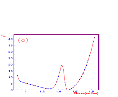
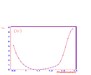
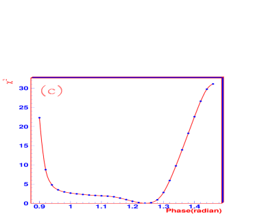
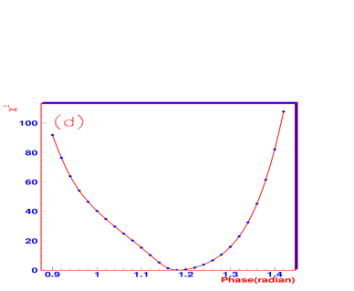
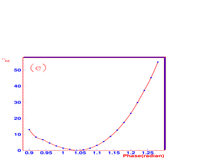
Figure 2: Scan results on I,J=0,0 phase. (a), (b), (c), (d) and (e) are scan results when D-component are 2%, 4%, 8%, 20% and 45% respectively. The value at minimum of the curve is the output phase.

Ratio of D-wave	2%	4%	8%	20%	45%
$\delta^{0}_{0}-\delta^{2}_{0}$	$1.28\pm 0.08$	$1.10\pm 0.16$	$1.24\pm 0.08$	$1.18\pm 0.04$	$1.04\pm 0.04$
	$1.52\pm 0.04$

Table 1: Scan results on $\delta^{0}_{0}-\delta^{2}_{0}$ for different D-wave components. Errors are only statistical. The input phase difference of Monte Carlo data are 1.03 for the 45% case and 1.17 for the rest.

Statistics of data is key important in the study of the phase difference. In the above study, the statistics of Monte Carlo data are 600,000, 250,000, 200,000, and 200,000 for D-wave component 2%, 4%, 8%, and 20% respectively. When the ratio of D-wave component is small, we need much higher statistics, otherwise likelihood function is not sensitive to the change of S-wave phase, or even not changed when S-wave phase is changed to any other value. In BESII data, there are only about 2,000 events in a 10 MeV bin when $m_{\pi\pi}$ is at 500 MeV. In these case, the fit is not at all sensitive to the phase shift difference. In the Monte Carlo study, we found similar results, that is, when D-wave component is 4% and statistics of the Monte Carlo data is below 10,000, the likelihood function almost kept unchanged when we change the S-wave phase to other value. Therefore, the reason that we can not obtain a reasonable result on S-wave phase shift is that the statistics of the BESII data is too few. It is expected that BESIII will collect 200 times more $\psi^{\prime}$ data in the near future. And BESIII detector has much higher selection efficiency than that of BESII detector. So, we will have more than 400,000 events in a 10 MeV bin when $m_{\pi\pi}$ is at 500 MeV. Our Monte Carlo study shows that, if the ratio of D-wave component is above 2%, a reasonable S-wave phase shift can be obtained based on BESIII data.

5 Conclusions

In this paper, a method is proposed to measure $\pi\pi$ S-wave phase shift, and this method is tested by Monte Carlo data. In the Monte Carlo study, it is found that, even if the ratio of the D-wave component is above 2% and the statistics in one 10 MeV bin is above about 200,000, a reasonable results on $\pi\pi$ S-wave phase shift can be obtained. It is expected that BESIII will collect enough data, so based on BESIII data, we can measure $\pi\pi$ S-wave phase shift in the mass region from 350 MeV to 550 MeV.

Acknowledgements: This work is support in part by National Nature Science Foundations of China under contract number 10575002,10491306 and 10721063, and by the EU-RTN Programme, Contract No MRTN-CT-2006-035482, ”Flavianet”.

Appendix A Kinematics

$\epsilon^{\prime}$ and $\epsilon$ denote the polarizations of $\Psi^{\prime}$ and $J/\Psi$ respectively. Here we choose

$$\epsilon_{0}^{\mu}=\frac{1}{M}(|\vec{p}_{3}|,0,0,-E_{3}),$$

$$\epsilon_{\pm}^{\mu}=\frac{\sqrt{2}}{2}(0,1,\pm i,0),$$

and

$$\epsilon^{{}^{\prime}\mu}_{1}=(0,-\cos\theta_{3}\cos\phi,-\cos\theta_{3}\sin\phi,-\sin\theta_{3}),$$

$$\epsilon^{{}^{\prime}\mu}_{2}=(0,-\sin\phi,\cos\phi,0).$$

$${p_{3}\cdot q}=\sqrt{s}(E_{3}+|\vec{p}_{3}|\beta),$$

$$p_{3}\cdot\epsilon^{\prime}_{1}=-|\vec{p}_{3}|\sin\theta_{3},$$

$$p\cdot\epsilon^{\prime}_{1}=2|\vec{p}_{\pi\pi}^{*}|(\cos\theta_{3}\cos\phi\sin\theta_{\pi}^{*}+\gamma\cos\theta_{\pi}^{*}\sin\theta_{3}),$$

$${q\cdot\epsilon^{\prime}_{1}}=\sqrt{s}\beta\gamma\sin\theta_{3},$$

$$p_{3}\cdot\epsilon^{\prime}_{2}=0,$$

$$p\cdot\epsilon^{\prime}_{2}=2|\vec{p}_{\pi\pi}^{*}|\sin\theta_{\pi}^{*}\sin\phi,$$

$$q\cdot\epsilon^{\prime}_{2}=0,$$

$$p\cdot\epsilon_{+}=-\sqrt{2}|\vec{p}_{\pi\pi}^{*}|\sin\theta_{\pi}^{*},$$

$$p\cdot\epsilon_{-}=-\sqrt{2}|\vec{p}_{\pi\pi}^{*}|\sin\theta_{\pi}^{*},$$

$$p\cdot\epsilon_{0}=2|\vec{p}_{\pi\pi}^{*}|\cos\theta_{\pi}^{*}\gamma(E_{3}+|\vec{p}_{3}|\beta)\frac{1}{M_{\Psi}},$$

$$q\cdot\epsilon_{+}=0,$$

$$q\cdot\epsilon_{-}=0,$$

$$q\cdot\epsilon_{0}=s\gamma(|\vec{p}_{3}|+E_{3}\beta)\frac{1}{M_{\Psi}}$$

$$\epsilon^{\prime}_{1}\cdot\epsilon_{+}=\cos\theta_{3}(\cos\phi+i\sin\phi)/\sqrt{2},$$

$$\epsilon^{\prime}_{1}\cdot\epsilon_{-}=\cos\theta_{3}(\cos\phi-i\sin\phi)/\sqrt{2},$$

$$\epsilon^{\prime}_{1}\cdot\epsilon_{0}=-E_{3}\sin\theta_{3}/M_{\Psi},$$

$$\epsilon^{\prime}_{2}\cdot\epsilon_{+}=(-i\cos\phi+\sin\phi)/\sqrt{2},$$

$$\epsilon^{\prime}_{2}\cdot\epsilon_{-}=(i\cos\phi+\sin\phi)/\sqrt{2},$$

$$\epsilon^{\prime}_{2}\cdot\epsilon_{0}=0.$$

Appendix B $G_{klm}$ and $\tilde{G}_{i}$

We have used the notations

$$P_{3}=|\vec{p}_{3}|,V=\beta,M=M_{J/\Psi},$$

and $\delta=\delta_{0}-\delta_{2}$ in the definitions of $G_{klm}$ and $\tilde{G}_{i}$  .

$$G_{224}=\frac{1}{M^{4}}(2{I_{3}}{I_{7}}\rho^{2}M^{4}+\rho^{4}(-{I_{6}}^{2}({P_{3}}+{E_{3}}V)^{4}\gamma^{4}-2{I_{6}}{I_{7}}M({P_{3}}+{E_{3}}V)^{2}({E_{3}}+{P_{3}}V)\gamma^{3}$$

$$+{I_{7}}^{2}M^{2}(M^{2}-({E_{3}}+{P_{3}}V)^{2}\gamma^{2}))),$$ (52)

$$G_{204}=-G_{224},$$ (53)

$$G_{222}=\frac{1}{3M^{4}}(\rho^{2}(3{I_{6}}^{2}\rho^{2}({P_{3}}+{E_{3}}V)^{4}\gamma^{4}-{I_{7}}^{2}M^{2}\rho^{2}(4M^{2}-3({E_{3}}+{P_{3}}V)^{2}\gamma^{2})$$

$$+2{I_{7}}M(3{\cos\delta}{I_{1}}M^{3}-4{I_{3}}M^{3}+3{I_{6}}\rho^{2}({P_{3}}+{E_{3}}V)^{2}({E_{3}}+{P_{3}}V)\gamma^{3}))),$$ (54)

$$G_{202}=-G_{222},$$ (55)

$$G_{220}=\frac{1}{3}{I_{7}}\rho^{2}({I_{7}}\rho^{2}-6{\cos\delta}{I_{1}}+2{I_{3}}),$$ (56)

$$G_{220}=-G_{200},$$ (57)

$$G_{024}=-\frac{1}{M^{4}}({E_{3}}^{4}({I_{5}}+{I_{6}})^{2}\rho^{4}V^{4}\gamma^{6}+2{E_{3}}^{3}({I_{5}}+{I_{6}})\rho^{2}V^{2}(\gamma^{2}({I_{7}}M\rho^{2}+V({P_{3}}({I_{5}}V^{2}+{I_{5}}+2{I_{6}})\gamma\rho^{2}+{I_{4}}MV))$$

$$-{I_{3}}M)\gamma^{3}+({I_{7}}^{2}M^{2}({P_{3}}^{2}V^{2}\gamma^{2}-M^{2})\rho^{4}+2{I_{7}}M{P_{3}}V\gamma({I_{5}}({P_{3}}^{2}V^{2}\gamma^{2}-M^{2})\rho^{2}+{P_{3}}\gamma({I_{6}}{P_{3}}\gamma\rho^{2}+{I_{4}}MV))\rho^{2}$$

$$+{P_{3}}^{2}\gamma^{2}((({P_{3}}^{2}V^{4}\gamma^{2}-M^{2}V^{2}){I_{5}}^{2}+2{I_{6}}{P_{3}}^{2}V^{2}\gamma^{2}{I_{5}}+{I_{6}}^{2}{P_{3}}^{2}\gamma^{2})\rho^{4}+2{I_{4}}M{P_{3}}V({I_{5}}V^{2}+{I_{6}})\gamma\rho^{2}+{I_{4}}^{2}M^{2}V^{2}))\gamma^{2}$$

$$+2{E_{3}}(\gamma({I_{5}}^{2}{P_{3}}V^{3}\gamma({P_{3}}^{2}(V^{2}+1)\gamma^{2}-M^{2})\rho^{4}+{I_{5}}V({I_{7}}MV({P_{3}}^{2}(V^{2}+2)\gamma^{2}-M^{2})\rho^{2}$$

$$+{P_{3}}^{2}\gamma^{2}({I_{6}}{P_{3}}(3V^{2}+1)\gamma\rho^{2}+{I_{4}}M(2V^{3}+V)))\rho^{2}+{P_{3}}\gamma(({I_{7}}^{2}VM^{2}+{I_{6}}{I_{7}}{P_{3}}(2V^{2}+1)\gamma M+2{I_{6}}^{2}{P_{3}}^{2}V\gamma^{2})\rho^{4}$$

$$+{I_{4}}MV({I_{7}}M(V^{2}+1)+3{I_{6}}{P_{3}}V\gamma)\rho^{2}+{I_{4}}^{2}M^{2}V^{3}))-{I_{3}}M{P_{3}}(({I_{7}}MV+{P_{3}}({I_{5}}V^{2}+{I_{6}})\gamma)\rho^{2}+{I_{4}}MV))\gamma^{2}$$

$$-{I_{3}}^{2}M^{4}+{E_{3}}^{2}(({I_{7}}^{2}M^{2}\rho^{4}+2{I_{7}}MV({P_{3}}(2{I_{5}}V^{2}+{I_{5}}+{I_{6}}(V^{2}+2))\gamma\rho^{2}+{I_{4}}MV)\rho^{2}$$

$$+V^{2}((({P_{3}}^{2}(V^{4}+4V^{2}+1)\gamma^{2}-M^{2}V^{2}){I_{5}}^{2}+6{I_{6}}{P_{3}}^{2}(V^{2}+1)\gamma^{2}{I_{5}}+6{I_{6}}^{2}{P_{3}}^{2}\gamma^{2})\rho^{4}+2{I_{4}}M{P_{3}}V(3{I_{6}}$$

$$+{I_{5}}(V^{2}+2))\gamma\rho^{2}+{I_{4}}^{2}M^{2}V^{2}))\gamma^{4}-2{I_{3}}M({I_{7}}M\rho^{2}+V({P_{3}}({I_{5}}V^{2}+{I_{5}}+2{I_{6}})\gamma\rho^{2}+{I_{4}}MV))\gamma^{2}+{I_{3}}^{2}M^{2})),$$ (58)

$$G_{004}=\frac{1}{M^{4}}({I_{6}}^{2}{P_{3}}^{4}\rho^{4}\gamma^{6}+{I_{5}}^{2}{P_{3}}^{4}\rho^{4}V^{4}\gamma^{6}+2{I_{5}}{I_{6}}{P_{3}}^{4}\rho^{4}V^{2}\gamma^{6}+2{I_{5}}{I_{7}}M{P_{3}}^{3}\rho^{4}V^{3}\gamma^{5}+2{I_{4}}{I_{5}}M{P_{3}}^{3}\rho^{2}V^{3}\gamma^{5}$$

$$+2{I_{6}}{I_{7}}M{P_{3}}^{3}\rho^{4}V\gamma^{5}+2{I_{4}}{I_{6}}M{P_{3}}^{3}\rho^{2}V\gamma^{5}-{I_{6}}^{2}{P_{3}}^{4}\rho^{4}\gamma^{4}-{I_{5}}^{2}M^{2}{P_{3}}^{2}\rho^{4}V^{2}\gamma^{4}+{I_{7}}^{2}M^{2}{P_{3}}^{2}\rho^{4}V^{2}\gamma^{4}$$

$$+{I_{4}}^{2}M^{2}{P_{3}}^{2}V^{2}\gamma^{4}+2{I_{4}}{I_{7}}M^{2}{P_{3}}^{2}\rho^{2}V^{2}\gamma^{4}+{E_{3}}^{4}\rho^{4}V^{4}((\gamma^{2}-1){I_{6}}^{2}+2{I_{5}}\gamma^{2}{I_{6}}+{I_{5}}^{2}\gamma^{2})\gamma^{4}-2{I_{6}}{I_{7}}M{P_{3}}^{3}\rho^{4}V\gamma^{3}$$

$$-2{I_{5}}{I_{7}}M^{3}{P_{3}}\rho^{4}V\gamma^{3}+2{E_{3}}^{3}\rho^{2}V^{2}(2{I_{6}}^{2}{P_{3}}V\gamma(\gamma^{2}-1)\rho^{2}-{I_{3}}({I_{5}}+{I_{6}})M+{I_{5}}\gamma^{2}({I_{7}}M\rho^{2}+V({I_{5}}{P_{3}}(V^{2}+1)\gamma\rho^{2}$$

$$+{I_{4}}MV))+{I_{6}}({I_{7}}M(\gamma^{2}-1)\rho^{2}+V\gamma^{2}({I_{5}}{P_{3}}(V^{2}+3)\gamma\rho^{2}+{I_{4}}MV)))\gamma^{3}-{I_{7}}^{2}M^{4}\rho^{4}\gamma^{2}-{I_{7}}^{2}M^{2}{P_{3}}^{2}\rho^{4}V^{2}\gamma^{2}$$

$$+2{E_{3}}({I_{7}}^{2}M^{2}{P_{3}}V(\gamma^{2}-1)\rho^{4}+{I_{7}}M\gamma({I_{6}}{P_{3}}^{2}(2V^{2}+1)(\gamma^{2}-1)\rho^{2}+V({I_{5}}V({P_{3}}^{2}(V^{2}+2)\gamma^{2}-M^{2})\rho^{2}$$

$$+{I_{4}}M{P_{3}}(V^{2}+1)\gamma))\rho^{2}-{I_{3}}M{P_{3}}(({I_{7}}MV+{P_{3}}({I_{5}}V^{2}+{I_{6}})\gamma)\rho^{2}+{I_{4}}MV)+{P_{3}}V\gamma^{2}(2{I_{6}}^{2}{P_{3}}^{2}(\gamma^{2}-1)\rho^{4}$$

$$+{I_{6}}{P_{3}}\gamma({I_{5}}{P_{3}}(3V^{2}+1)\gamma\rho^{2}+3{I_{4}}MV)\rho^{2}+V({I_{5}}^{2}V({P_{3}}^{2}(V^{2}+1)\gamma^{2}-M^{2})\rho^{4}+{I_{4}}{I_{5}}M{P_{3}}(2V^{2}+1)\gamma\rho^{2}$$

$$+{I_{4}}^{2}M^{2}V)))\gamma^{2}+{I_{3}}^{2}M^{4}+{I_{7}}^{2}M^{4}\rho^{4}+2{I_{3}}{I_{7}}M^{4}\rho^{2}+{E_{3}}^{2}({I_{3}}^{2}M^{2}-2{I_{3}}\gamma^{2}({I_{7}}M\rho^{2}+V({P_{3}}({I_{5}}V^{2}+{I_{5}}+2{I_{6}})\gamma\rho^{2}$$

$$+{I_{4}}MV))M+\gamma^{2}({I_{7}}^{2}M^{2}(\gamma^{2}-1)\rho^{4}+2{I_{7}}MV\gamma({I_{6}}{P_{3}}(V^{2}+2)(\gamma^{2}-1)\rho^{2}+\gamma({I_{5}}{P_{3}}(2V^{2}+1)\gamma\rho^{2}+{I_{4}}MV))\rho^{2}$$

$$+V^{2}\gamma^{2}(6{I_{6}}^{2}{P_{3}}^{2}(\gamma^{2}-1)\rho^{4}+{I_{5}}^{2}({P_{3}}^{2}(V^{4}+4V^{2}+1)\gamma^{2}-M^{2}V^{2})\rho^{4}+2{I_{4}}{I_{5}}M{P_{3}}V(V^{2}+2)\gamma\rho^{2}$$

$$+6{I_{6}}{P_{3}}\gamma({I_{5}}{P_{3}}(V^{2}+1)\gamma\rho^{2}+{I_{4}}MV)\rho^{2}+{I_{4}}^{2}M^{2}V^{2})))),$$ (59)

$$G_{022}=\frac{1}{3M^{4}}(2{I_{5}}^{2}{P_{3}}^{4}\rho^{4}V^{4}\gamma^{6}+2{I_{5}}{I_{6}}{P_{3}}^{4}\rho^{4}V^{4}\gamma^{6}+2{E_{3}}^{4}({I_{5}}+{I_{6}})^{2}\rho^{4}V^{4}\gamma^{6}+2{I_{6}}^{2}{P_{3}}^{4}\rho^{4}V^{2}\gamma^{6}+2{I_{5}}{I_{6}}{P_{3}}^{4}\rho^{4}V^{2}\gamma^{6}$$

$$+4{I_{5}}{I_{7}}M{P_{3}}^{3}\rho^{4}V^{3}\gamma^{5}+2{I_{6}}{I_{7}}M{P_{3}}^{3}\rho^{4}V^{3}\gamma^{5}+4{I_{4}}{I_{5}}M{P_{3}}^{3}\rho^{2}V^{3}\gamma^{5}+2{I_{4}}{I_{6}}M{P_{3}}^{3}\rho^{2}V^{3}\gamma^{5}+2{I_{6}}{I_{7}}M{P_{3}}^{3}\rho^{4}V\gamma^{5}$$

$$+2{I_{4}}{I_{6}}M{P_{3}}^{3}\rho^{2}V\gamma^{5}+2{I_{6}}^{2}{P_{3}}^{4}\rho^{4}\gamma^{4}+2{I_{5}}{I_{6}}{P_{3}}^{4}\rho^{4}V^{2}\gamma^{4}-3{I_{5}}^{2}M^{2}{P_{3}}^{2}\rho^{4}V^{2}\gamma^{4}+2{I_{7}}^{2}M^{2}{P_{3}}^{2}\rho^{4}V^{2}\gamma^{4}$$

$$+2{I_{4}}^{2}M^{2}{P_{3}}^{2}V^{2}\gamma^{4}+4{I_{4}}{I_{7}}M^{2}{P_{3}}^{2}\rho^{2}V^{2}\gamma^{4}+2{I_{6}}{I_{7}}M{P_{3}}^{3}\rho^{4}V\gamma^{3}-6{I_{5}}{I_{7}}M^{3}{P_{3}}\rho^{4}V\gamma^{3}+2{I_{4}}{I_{6}}M{P_{3}}^{3}\rho^{2}V\gamma^{3}$$

$$+2{E_{3}}^{3}({I_{5}}+{I_{6}})\rho^{2}V^{2}({I_{7}}M((V^{2}+1)\gamma^{2}+1)\rho^{2}-2{I_{3}}M+V\gamma({I_{6}}{P_{3}}((V^{2}+3)\gamma^{2}+1)\rho^{2}+2\gamma({I_{5}}{P_{3}}(V^{2}+1)\gamma\rho^{2}$$

$$+{I_{4}}MV)))\gamma^{3}-3{I_{7}}^{2}M^{4}\rho^{4}\gamma^{2}+2{E_{3}}(\gamma(({I_{7}}^{2}{P_{3}}V((V^{2}+1)\gamma^{2}+1)M^{2}+{I_{7}}\gamma({I_{6}}(\gamma^{2}V^{4}+(5\gamma^{2}+1)V^{2}+2){P_{3}}^{2}$$

$$+{I_{5}}V^{2}({P_{3}}^{2}(3(V^{2}+1)\gamma^{2}+1)-3M^{2}))M+{P_{3}}V\gamma^{2}({I_{6}}^{2}((3V^{2}+1)\gamma^{2}+3){P_{3}}^{2}+{I_{5}}{I_{6}}(2\gamma^{2}V^{4}+(5\gamma^{2}+2)V^{2}+\gamma^{2}$$

$$+1){P_{3}}^{2}+{I_{5}}^{2}V^{2}(2{P_{3}}^{2}(V^{2}+1)\gamma^{2}-3M^{2})))\rho^{4}+{I_{4}}M{P_{3}}V({I_{7}}M((3V^{2}+1)\gamma^{2}+1)+2{P_{3}}V\gamma({I_{5}}(2V^{2}+1)\gamma^{2}$$

$$+{I_{6}}((V^{2}+2)\gamma^{2}+1)))\rho^{2}+2{I_{4}}^{2}M^{2}{P_{3}}V^{3}\gamma^{2})-{I_{3}}M{P_{3}}({I_{6}}{P_{3}}((V^{2}+1)\gamma^{2}+1)\rho^{2}+2V\gamma(({I_{7}}M+{I_{5}}{P_{3}}V\gamma)\rho^{2}$$

$$+{I_{4}}M)))\gamma-2{I_{3}}^{2}M^{4}+2{I_{3}}{I_{7}}M^{4}\rho^{2}+6{\cos\delta}M(-{I_{2}}{P_{3}}^{2}V(({I_{7}}MV+{P_{3}}({I_{5}}V^{2}+{I_{6}})\gamma)\rho^{2}+{I_{4}}MV)\gamma^{4}$$

$$+{E_{3}}^{3}({I_{5}}+{I_{6}})\rho^{2}V^{2}({I_{1}}-{I_{2}}V^{2}\gamma^{2})\gamma^{3}+{E_{3}}{P_{3}}({I_{1}}(({I_{7}}MV+{P_{3}}({I_{5}}V^{2}+{I_{6}})\gamma)\rho^{2}+{I_{4}}MV)-{I_{2}}V(\gamma^{2}({I_{7}}M(V^{2}$$

$$+1)\rho^{2}+V({P_{3}}(2{I_{5}}V^{2}+{I_{5}}+3{I_{6}})\gamma\rho^{2}+2{I_{4}}MV))-{I_{3}}M))\gamma^{2}+{I_{1}}{I_{3}}M^{3}+{E_{3}}^{2}({I_{1}}(\gamma^{2}({I_{7}}M\rho^{2}$$

$$+V({P_{3}}({I_{5}}V^{2}+{I_{5}}+2{I_{6}})\gamma\rho^{2}+{I_{4}}MV))-{I_{3}}M)-{I_{2}}V^{2}\gamma^{2}(\gamma^{2}({I_{7}}M\rho^{2}+V({P_{3}}(3{I_{6}}+{I_{5}}(V^{2}+2))\gamma\rho^{2}+{I_{4}}MV))$$

$$-{I_{3}}M)))+{E_{3}}^{2}(2{I_{3}}^{2}M^{2}-2{I_{3}}({I_{7}}M((V^{2}+1)\gamma^{2}+1)\rho^{2}+V\gamma({I_{6}}{P_{3}}((V^{2}+3)\gamma^{2}+1)\rho^{2}+2\gamma({I_{5}}{P_{3}}(V^{2}+1)\gamma\rho^{2}$$

$$+{I_{4}}MV)))M+\gamma^{2}(2{I_{7}}^{2}M^{2}(V^{2}\gamma^{2}+1)\rho^{4}+2{I_{7}}MV({P_{3}}\gamma({I_{6}}(5V^{2}\gamma^{2}+\gamma^{2}+3)+{I_{5}}(\gamma^{2}V^{4}+4\gamma^{2}V^{2}+V^{2}$$

$$+\gamma^{2}+1))\rho^{2}+{I_{4}}MV((V^{2}+1)\gamma^{2}+1))\rho^{2}+V^{2}\gamma(\gamma((2{P_{3}}^{2}(V^{4}+4V^{2}+1)\gamma^{2}-3M^{2}V^{2}){I_{5}}^{2}+2{I_{6}}{P_{3}}^{2}(\gamma^{2}V^{4}$$

$$+(7\gamma^{2}+1)V^{2}+4\gamma^{2}+2){I_{5}}+6{I_{6}}^{2}{P_{3}}^{2}((V^{2}+1)\gamma^{2}+1))\rho^{4}+2{I_{4}}M{P_{3}}V(2{I_{5}}(V^{2}+2)\gamma^{2}$$

$$+{I_{6}}((V^{2}+5)\gamma^{2}+1))\rho^{2}+2{I_{4}}^{2}M^{2}V^{2}\gamma)))),$$ (60)

$$G_{002}=-\frac{1}{3M^{4}}(2{I_{5}}^{2}{P_{3}}^{4}\rho^{4}V^{4}\gamma^{6}+2{I_{5}}{I_{6}}{P_{3}}^{4}\rho^{4}V^{4}\gamma^{6}+2{I_{6}}^{2}{P_{3}}^{4}\rho^{4}V^{2}\gamma^{6}+2{I_{5}}{I_{6}}{P_{3}}^{4}\rho^{4}V^{2}\gamma^{6}+4{I_{5}}{I_{7}}M{P_{3}}^{3}\rho^{4}V^{3}\gamma^{5}$$

$$+2{I_{6}}{I_{7}}M{P_{3}}^{3}\rho^{4}V^{3}\gamma^{5}+4{I_{4}}{I_{5}}M{P_{3}}^{3}\rho^{2}V^{3}\gamma^{5}+2{I_{4}}{I_{6}}M{P_{3}}^{3}\rho^{2}V^{3}\gamma^{5}+2{I_{6}}{I_{7}}M{P_{3}}^{3}\rho^{4}V\gamma^{5}+2{I_{4}}{I_{6}}M{P_{3}}^{3}\rho^{2}V\gamma^{5}$$

$$-{I_{6}}^{2}{P_{3}}^{4}\rho^{4}\gamma^{4}+2{I_{5}}{I_{6}}{P_{3}}^{4}\rho^{4}V^{2}\gamma^{4}-3{I_{5}}^{2}M^{2}{P_{3}}^{2}\rho^{4}V^{2}\gamma^{4}+2{I_{7}}^{2}M^{2}{P_{3}}^{2}\rho^{4}V^{2}\gamma^{4}+2{I_{4}}^{2}M^{2}{P_{3}}^{2}V^{2}\gamma^{4}$$

$$+4{I_{4}}{I_{7}}M^{2}{P_{3}}^{2}\rho^{2}V^{2}\gamma^{4}+{E_{3}}^{4}\rho^{4}V^{4}((2\gamma^{2}-3){I_{6}}^{2}+4{I_{5}}\gamma^{2}{I_{6}}+2{I_{5}}^{2}\gamma^{2})\gamma^{4}-4{I_{6}}{I_{7}}M{P_{3}}^{3}\rho^{4}V\gamma^{3}-6{I_{5}}{I_{7}}M^{3}{P_{3}}\rho^{4}V\gamma^{3}$$

$$+2{I_{4}}{I_{6}}M{P_{3}}^{3}\rho^{2}V\gamma^{3}+2{E_{3}}^{3}\rho^{2}V^{2}(2{I_{5}}^{2}{P_{3}}\rho^{2}V(V^{2}+1)\gamma^{3}-2{I_{3}}({I_{5}}+{I_{6}})M+{I_{6}}({I_{7}}M((V^{2}+1)\gamma^{2}-2)\rho^{2}$$

$$+V\gamma({I_{6}}{P_{3}}((V^{2}+3)\gamma^{2}-5)\rho^{2}+2{I_{4}}MV\gamma))+{I_{5}}({I_{7}}M((V^{2}+1)\gamma^{2}+1)\rho^{2}+V\gamma({I_{6}}{P_{3}}((3V^{2}+5)\gamma^{2}+1)\rho^{2}$$

$$+2{I_{4}}MV\gamma)))\gamma^{3}-3{I_{7}}^{2}M^{4}\rho^{4}\gamma^{2}-3{I_{7}}^{2}M^{2}{P_{3}}^{2}\rho^{4}V^{2}\gamma^{2}+2{E_{3}}(\gamma(({I_{7}}^{2}{P_{3}}V((V^{2}+1)\gamma^{2}-2)M^{2}+{I_{7}}\gamma({I_{6}}(\gamma^{2}V^{4}$$

$$+5(\gamma^{2}-1)V^{2}-1){P_{3}}^{2}+{I_{5}}V^{2}({P_{3}}^{2}(3(V^{2}+1)\gamma^{2}+1)-3M^{2}))M+{P_{3}}V\gamma^{2}({I_{6}}^{2}((3V^{2}+1)\gamma^{2}-3){P_{3}}^{2}$$

$$+{I_{5}}{I_{6}}(2\gamma^{2}V^{4}+(5\gamma^{2}+2)V^{2}+\gamma^{2}+1){P_{3}}^{2}+{I_{5}}^{2}V^{2}(2{P_{3}}^{2}(V^{2}+1)\gamma^{2}-3M^{2})))\rho^{4}+{I_{4}}M{P_{3}}V({I_{7}}M((3V^{2}+1)\gamma^{2}$$

$$+1)+2{P_{3}}V\gamma({I_{5}}(2V^{2}+1)\gamma^{2}+{I_{6}}((V^{2}+2)\gamma^{2}+1)))\rho^{2}+2{I_{4}}^{2}M^{2}{P_{3}}V^{3}\gamma^{2})-{I_{3}}M{P_{3}}({I_{6}}{P_{3}}((V^{2}+1)\gamma^{2}+1)\rho^{2}$$

$$+2V\gamma(({I_{7}}M+{I_{5}}{P_{3}}V\gamma)\rho^{2}+{I_{4}}M)))\gamma+2{I_{3}}^{2}M^{4}+4{I_{7}}^{2}M^{4}\rho^{4}+6{I_{3}}{I_{7}}M^{4}\rho^{2}$$

$$-6{\cos\delta}M({I_{2}}{P_{3}}^{2}V(({I_{7}}MV+{P_{3}}({I_{5}}V^{2}+{I_{6}})\gamma)\rho^{2}+{I_{4}}MV)\gamma^{4}+{E_{3}}^{3}({I_{5}}+{I_{6}})\rho^{2}V^{2}({I_{2}}V^{2}\gamma^{2}-{I_{1}})\gamma^{3}$$

$$+{E_{3}}{P_{3}}({I_{2}}V(\gamma^{2}({I_{7}}M(V^{2}+1)\rho^{2}+V({P_{3}}(2{I_{5}}V^{2}+{I_{5}}+3{I_{6}})\gamma\rho^{2}+2{I_{4}}MV))-{I_{3}}M)$$

$$-{I_{1}}(({I_{7}}MV+{P_{3}}({I_{5}}V^{2}+{I_{6}})\gamma)\rho^{2}+{I_{4}}MV))\gamma^{2}+{I_{1}}M^{3}({I_{7}}\rho^{2}+{I_{3}})+{E_{3}}^{2}({I_{2}}V^{2}(\gamma^{2}({I_{7}}M\rho^{2}+V({P_{3}}(3{I_{6}}$$

$$+{I_{5}}(V^{2}+2))\gamma\rho^{2}+{I_{4}}MV))-{I_{3}}M)\gamma^{2}+{I_{1}}({I_{3}}M-\gamma^{2}({I_{7}}M\rho^{2}+V({P_{3}}({I_{5}}V^{2}+{I_{5}}+2{I_{6}})\gamma\rho^{2}+{I_{4}}MV)))))$$

$$+{E_{3}}^{2}(2{I_{3}}^{2}M^{2}-2{I_{3}}({I_{7}}M((V^{2}+1)\gamma^{2}+1)\rho^{2}+V\gamma({I_{6}}{P_{3}}((V^{2}+3)\gamma^{2}+1)\rho^{2}$$

$$+2\gamma({I_{5}}{P_{3}}(V^{2}+1)\gamma\rho^{2}+{I_{4}}MV)))M+\gamma^{2}({I_{7}}^{2}M^{2}(2V^{2}\gamma^{2}-1)\rho^{4}$$

$$+2{I_{7}}MV({P_{3}}\gamma({I_{5}}(\gamma^{2}V^{4}+(4\gamma^{2}+1)V^{2}+\gamma^{2}+1)+{I_{6}}((5\gamma^{2}-3)V^{2}+\gamma^{2}-3))\rho^{2}$$

$$+{I_{4}}MV((V^{2}+1)\gamma^{2}+1))\rho^{2}+V^{2}\gamma(\gamma((2{P_{3}}^{2}(V^{4}+4V^{2}+1)\gamma^{2}-3M^{2}V^{2}){I_{5}}^{2}$$

$$+2{I_{6}}{P_{3}}^{2}(\gamma^{2}V^{4}+(7\gamma^{2}+1)V^{2}+4\gamma^{2}{I_{5}}+6{I_{6}}^{2}{P_{3}}^{2}((V^{2}+1)\gamma^{2}-2))\rho^{4}$$

$$+2{I_{4}}M{P_{3}}V(2{I_{5}}(V^{2}+2)\gamma^{2}+{I_{6}}((V^{2}+5)\gamma^{2}+1))\rho^{2}+2{I_{4}}^{2}M^{2}V^{2}\gamma))))),$$ (61)

$$G_{020}=-\frac{1}{9M^{4}}({I_{5}}^{2}{P_{3}}^{4}\rho^{4}V^{4}\gamma^{6}+{I_{6}}^{2}{P_{3}}^{4}\rho^{4}V^{4}\gamma^{6}+2{I_{5}}{I_{6}}{P_{3}}^{4}\rho^{4}V^{4}\gamma^{6}+{E_{3}}^{4}({I_{5}}+{I_{6}})^{2}\rho^{4}V^{4}\gamma^{6}+2{I_{5}}{I_{7}}M{P_{3}}^{3}\rho^{4}V^{3}\gamma^{5}$$

$$+2{I_{6}}{I_{7}}M{P_{3}}^{3}\rho^{4}V^{3}\gamma^{5}-6{\cos\delta}{I_{2}}{I_{5}}M{P_{3}}^{3}\rho^{2}V^{3}\gamma^{5}+2{I_{4}}{I_{5}}M{P_{3}}^{3}\rho^{2}V^{3}\gamma^{5}-6{\cos\delta}{I_{2}}{I_{6}}M{P_{3}}^{3}\rho^{2}V^{3}\gamma^{5}$$

$$+2{I_{4}}{I_{6}}M{P_{3}}^{3}\rho^{2}V^{3}\gamma^{5}+2{I_{6}}^{2}{P_{3}}^{4}\rho^{4}V^{2}\gamma^{4}+2{I_{5}}{I_{6}}{P_{3}}^{4}\rho^{4}V^{2}\gamma^{4}+{I_{7}}^{2}M^{2}{P_{3}}^{2}\rho^{4}V^{2}\gamma^{4}+9{I_{2}}^{2}M^{2}{P_{3}}^{2}V^{2}\gamma^{4}$$

$$+{I_{4}}^{2}M^{2}{P_{3}}^{2}V^{2}\gamma^{4}-6{\cos\delta}{I_{2}}{I_{4}}M^{2}{P_{3}}^{2}V^{2}\gamma^{4}-6{\cos\delta}{I_{2}}{I_{7}}M^{2}{P_{3}}^{2}\rho^{2}V^{2}\gamma^{4}+2{I_{4}}{I_{7}}M^{2}{P_{3}}^{2}\rho^{2}V^{2}\gamma^{4}$$

$$+2{I_{6}}{I_{7}}M{P_{3}}^{3}\rho^{4}V\gamma^{3}-6{\cos\delta}{I_{2}}{I_{6}}M{P_{3}}^{3}\rho^{2}V\gamma^{3}+2{I_{4}}{I_{6}}M{P_{3}}^{3}\rho^{2}V\gamma^{3}+2{E_{3}}^{3}({I_{5}}+{I_{6}})\rho^{2}V^{2}({I_{5}}{P_{3}}\rho^{2}V^{3}\gamma^{3}$$

$$+{I_{6}}{P_{3}}\rho^{2}V^{3}\gamma^{3}+{I_{5}}{P_{3}}\rho^{2}V\gamma^{3}+{I_{6}}{P_{3}}\rho^{2}V\gamma^{3}+{I_{7}}M\rho^{2}V^{2}\gamma^{2}+{I_{4}}MV^{2}\gamma^{2}+{I_{6}}{P_{3}}\rho^{2}V\gamma+{I_{7}}M\rho^{2}$$

$$-{I_{3}}M+3{\cos\delta}M({I_{1}}-{I_{2}}V^{2}\gamma^{2}))\gamma^{3}+{I_{6}}^{2}{P_{3}}^{4}\rho^{4}\gamma^{2}+2{E_{3}}{P_{3}}({I_{5}}^{2}{P_{3}}^{2}\rho^{4}V^{5}\gamma^{5}+{I_{6}}^{2}{P_{3}}^{2}\rho^{4}V^{5}\gamma^{5}$$

$$+2{I_{5}}{I_{6}}{P_{3}}^{2}\rho^{4}V^{5}\gamma^{5}+{I_{5}}^{2}{P_{3}}^{2}\rho^{4}V^{3}\gamma^{5}+{I_{6}}^{2}{P_{3}}^{2}\rho^{4}V^{3}\gamma^{5}+2{I_{5}}{I_{6}}{P_{3}}^{2}\rho^{4}V^{3}\gamma^{5}+2{I_{5}}{I_{7}}M{P_{3}}\rho^{4}V^{4}\gamma^{4}$$

$$+2{I_{6}}{I_{7}}M{P_{3}}\rho^{4}V^{4}\gamma^{4}+2{I_{4}}{I_{5}}M{P_{3}}\rho^{2}V^{4}\gamma^{4}+2{I_{4}}{I_{6}}M{P_{3}}\rho^{2}V^{4}\gamma^{4}+{I_{5}}{I_{7}}M{P_{3}}\rho^{4}V^{2}\gamma^{4}+{I_{6}}{I_{7}}M{P_{3}}\rho^{4}V^{2}\gamma^{4}$$

$$+{I_{4}}{I_{5}}M{P_{3}}\rho^{2}V^{2}\gamma^{4}+{I_{4}}{I_{6}}M{P_{3}}\rho^{2}V^{2}\gamma^{4}+{I_{7}}^{2}M^{2}\rho^{4}V^{3}\gamma^{3}+2{I_{6}}^{2}{P_{3}}^{2}\rho^{4}V^{3}\gamma^{3}+2{I_{5}}{I_{6}}{P_{3}}^{2}\rho^{4}V^{3}\gamma^{3}$$

$$+9{I_{2}}^{2}M^{2}V^{3}\gamma^{3}+{I_{4}}^{2}M^{2}V^{3}\gamma^{3}+2{I_{4}}{I_{7}}M^{2}\rho^{2}V^{3}\gamma^{3}+{I_{6}}^{2}{P_{3}}^{2}\rho^{4}V\gamma^{3}+{I_{5}}{I_{6}}{P_{3}}^{2}\rho^{4}V\gamma^{3}+{I_{5}}{I_{7}}M{P_{3}}\rho^{4}V^{2}\gamma^{2}$$

$$+3{I_{6}}{I_{7}}M{P_{3}}\rho^{4}V^{2}\gamma^{2}+2{I_{4}}{I_{6}}M{P_{3}}\rho^{2}V^{2}\gamma^{2}+{I_{7}}^{2}M^{2}\rho^{4}V\gamma+{I_{6}}^{2}{P_{3}}^{2}\rho^{4}V\gamma-9{I_{1}}{I_{2}}M^{2}V\gamma$$

$$+{I_{4}}{I_{7}}M^{2}\rho^{2}V\gamma+{I_{6}}{I_{7}}M{P_{3}}\rho^{4}-{I_{3}}M({I_{6}}{P_{3}}(V^{2}\gamma^{2}+1)\rho^{2}+V\gamma(({I_{7}}M+{I_{5}}{P_{3}}V\gamma)\rho^{2}+{I_{4}}M))$$

$$+3{\cos\delta}M({I_{1}}({I_{6}}{P_{3}}(V^{2}\gamma^{2}+1)\rho^{2}+V\gamma(({I_{7}}M+{I_{5}}{P_{3}}V\gamma)\rho^{2}+{I_{4}}M))-{I_{2}}V\gamma({I_{7}}M(2V^{2}\gamma^{2}+1)\rho^{2}$$

$$-{I_{3}}M+V\gamma({I_{6}}{P_{3}}((2V^{2}+1)\gamma^{2}+2)\rho^{2}+\gamma({I_{5}}{P_{3}}(2V^{2}+1)\gamma\rho^{2}+2{I_{4}}MV)))))\gamma-9{I_{1}}^{2}M^{4}$$

$$-{I_{3}}^{2}M^{4}-{I_{7}}^{2}M^{4}\rho^{4}+2{I_{3}}{I_{7}}M^{4}\rho^{2}+6{\cos\delta}{I_{1}}M^{4}({I_{3}}-{I_{7}}\rho^{2})+{E_{3}}^{2}({I_{5}}^{2}{P_{3}}^{2}\rho^{4}V^{6}\gamma^{6}+{I_{6}}^{2}{P_{3}}^{2}\rho^{4}V^{6}\gamma^{6}$$

$$+2{I_{5}}{I_{6}}{P_{3}}^{2}\rho^{4}V^{6}\gamma^{6}+4{I_{5}}^{2}{P_{3}}^{2}\rho^{4}V^{4}\gamma^{6}+4{I_{6}}^{2}{P_{3}}^{2}\rho^{4}V^{4}\gamma^{6}+8{I_{5}}{I_{6}}{P_{3}}^{2}\rho^{4}V^{4}\gamma^{6}+{I_{5}}^{2}{P_{3}}^{2}\rho^{4}V^{2}\gamma^{6}$$

$$+{I_{6}}^{2}{P_{3}}^{2}\rho^{4}V^{2}\gamma^{6}+2{I_{5}}{I_{6}}{P_{3}}^{2}\rho^{4}V^{2}\gamma^{6}+2{I_{5}}{I_{7}}M{P_{3}}\rho^{4}V^{5}\gamma^{5}+2{I_{6}}{I_{7}}M{P_{3}}\rho^{4}V^{5}\gamma^{5}$$

$$-6{\cos\delta}{I_{2}}{I_{5}}M{P_{3}}\rho^{2}V^{5}\gamma^{5}+2{I_{4}}{I_{5}}M{P_{3}}\rho^{2}V^{5}\gamma^{5}-6{\cos\delta}{I_{2}}{I_{6}}M{P_{3}}\rho^{2}V^{5}\gamma^{5}+2{I_{4}}{I_{6}}M{P_{3}}\rho^{2}V^{5}\gamma^{5}$$

$$+4{I_{5}}{I_{7}}M{P_{3}}\rho^{4}V^{3}\gamma^{5}+4{I_{6}}{I_{7}}M{P_{3}}\rho^{4}V^{3}\gamma^{5}-12{\cos\delta}{I_{2}}{I_{5}}M{P_{3}}\rho^{2}V^{3}\gamma^{5}+4{I_{4}}{I_{5}}M{P_{3}}\rho^{2}V^{3}\gamma^{5}$$

$$-12{\cos\delta}{I_{2}}{I_{6}}M{P_{3}}\rho^{2}V^{3}\gamma^{5}+4{I_{4}}{I_{6}}M{P_{3}}\rho^{2}V^{3}\gamma^{5}+{I_{7}}^{2}M^{2}\rho^{4}V^{4}\gamma^{4}+2{I_{6}}^{2}{P_{3}}^{2}\rho^{4}V^{4}\gamma^{4}$$

$$+2{I_{5}}{I_{6}}{P_{3}}^{2}\rho^{4}V^{4}\gamma^{4}+9{I_{2}}^{2}M^{2}V^{4}\gamma^{4}+{I_{4}}^{2}M^{2}V^{4}\gamma^{4}-6{\cos\delta}{I_{2}}{I_{4}}M^{2}V^{4}\gamma^{4}-6{\cos\delta}{I_{2}}{I_{7}}M^{2}\rho^{2}V^{4}\gamma^{4}$$

$$+2{I_{4}}{I_{7}}M^{2}\rho^{2}V^{4}\gamma^{4}+4{I_{6}}^{2}{P_{3}}^{2}\rho^{4}V^{2}\gamma^{4}+4{I_{5}}{I_{6}}{P_{3}}^{2}\rho^{4}V^{2}\gamma^{4}+2{I_{5}}{I_{7}}M{P_{3}}\rho^{4}V^{3}\gamma^{3}+4{I_{6}}{I_{7}}M{P_{3}}\rho^{4}V^{3}\gamma^{3}$$

$$-6{\cos\delta}{I_{2}}{I_{6}}M{P_{3}}\rho^{2}V^{3}\gamma^{3}+2{I_{4}}{I_{6}}M{P_{3}}\rho^{2}V^{3}\gamma^{3}+2{I_{5}}{I_{7}}M{P_{3}}\rho^{4}V\gamma^{3}+2{I_{6}}{I_{7}}M{P_{3}}\rho^{4}V\gamma^{3}$$

$$+2{I_{7}}^{2}M^{2}\rho^{4}V^{2}\gamma^{2}+{I_{6}}^{2}{P_{3}}^{2}\rho^{4}V^{2}\gamma^{2}-6{\cos\delta}{I_{2}}{I_{7}}M^{2}\rho^{2}V^{2}\gamma^{2}+2{I_{4}}{I_{7}}M^{2}\rho^{2}V^{2}\gamma^{2}+2{I_{6}}{I_{7}}M{P_{3}}\rho^{4}V\gamma$$

$$+{I_{7}}^{2}M^{2}\rho^{4}+9{I_{1}}^{2}M^{2}+{I_{3}}^{2}M^{2}-2{I_{3}}M({I_{7}}M(V^{2}\gamma^{2}+1)\rho^{2}+V\gamma({I_{6}}{P_{3}}((V^{2}+1)\gamma^{2}+1)\rho^{2}$$

$$+\gamma({I_{5}}{P_{3}}(V^{2}+1)\gamma\rho^{2}-3{\cos\delta}{I_{2}}MV+{I_{4}}MV)))+6{I_{1}}M({\cos\delta}({I_{7}}M(V^{2}\gamma^{2}+1)\rho^{2}-{I_{3}}M$$

$$+V\gamma({I_{6}}{P_{3}}((V^{2}+1)\gamma^{2}+1)\rho^{2}+\gamma({I_{5}}{P_{3}}(V^{2}+1)\gamma\rho^{2}+{I_{4}}MV)))-3{I_{2}}MV^{2}\gamma^{2}))),$$ (62)

$$G_{000}=\frac{1}{9M^{4}s}({I_{5}}^{2}{P_{3}}^{4}\rho^{4}sV^{4}\gamma^{6}+{I_{6}}^{2}{P_{3}}^{4}\rho^{4}sV^{4}\gamma^{6}+2{I_{5}}{I_{6}}{P_{3}}^{4}\rho^{4}sV^{4}\gamma^{6}+{E_{3}}^{4}({I_{5}}+{I_{6}})^{2}\rho^{4}sV^{4}\gamma^{6}$$

$$-6{\cos\delta}{I_{2}}{I_{5}}M{P_{3}}^{3}\rho^{2}sV^{3}\gamma^{5}+2{I_{4}}{I_{5}}M{P_{3}}^{3}\rho^{2}sV^{3}\gamma^{5}-6{\cos\delta}{I_{2}}{I_{6}}M{P_{3}}^{3}\rho^{2}sV^{3}\gamma^{5}+2{I_{4}}{I_{6}}M{P_{3}}^{3}\rho^{2}sV^{3}\gamma^{5}$$

$$+2{I_{6}}^{2}{P_{3}}^{4}\rho^{4}sV^{2}\gamma^{4}+2{I_{5}}{I_{6}}{P_{3}}^{4}\rho^{4}sV^{2}\gamma^{4}+9{I_{2}}^{2}M^{2}{P_{3}}^{2}sV^{2}\gamma^{4}+{I_{4}}^{2}M^{2}{P_{3}}^{2}sV^{2}\gamma^{4}$$

$$-6{\cos\delta}{I_{2}}{I_{4}}M^{2}{P_{3}}^{2}sV^{2}\gamma^{4}-6{\cos\delta}{I_{2}}{I_{6}}M{P_{3}}^{3}\rho^{2}sV\gamma^{3}+2{I_{4}}{I_{6}}M{P_{3}}^{3}\rho^{2}sV\gamma^{3}$$

$$+2{E_{3}}^{3}({I_{5}}+{I_{6}})\rho^{2}V^{2}(-{I_{3}}Ms+3{\cos\delta}M({I_{1}}-{I_{2}}V^{2}\gamma^{2})s+V\gamma({P_{3}}({I_{5}}s(V^{2}+1)\gamma^{2}+{I_{6}}s((V^{2}+1)\gamma^{2}+1))\rho^{2}$$

$$+{I_{4}}MsV\gamma))\gamma^{3}+{I_{6}}^{2}{P_{3}}^{4}\rho^{4}s\gamma^{2}+2{E_{3}}{P_{3}}s({P_{3}}^{2}V\gamma({I_{5}}^{2}V^{2}(V^{2}+1)\gamma^{4}+{I_{5}}{I_{6}}(2\gamma^{2}V^{4}+2(\gamma^{2}+1)V^{2}+1)\gamma^{2}$$

$$+{I_{6}}^{2}((V^{4}+V^{2})\gamma^{4}+(2V^{2}+1)\gamma^{2}+1))\rho^{4}+M{P_{3}}({I_{4}}V^{2}({I_{5}}(2V^{2}+1)\gamma^{2}+{I_{6}}(2V^{2}\gamma^{2}+\gamma^{2}+2))\gamma^{2}$$

$$-{I_{3}}({I_{5}}V^{2}\gamma^{2}+{I_{6}}V^{2}\gamma^{2}+{I_{6}})+3{\cos\delta}({I_{1}}({I_{5}}V^{2}\gamma^{2}+{I_{6}}V^{2}\gamma^{2}+{I_{6}})-{I_{2}}V^{2}\gamma^{2}({I_{5}}(2V^{2}+1)\gamma^{2}$$

$$+{I_{6}}(2V^{2}\gamma^{2}+\gamma^{2}+2))))\rho^{2}+M^{2}V\gamma(9{I_{2}}^{2}V^{2}\gamma^{2}+{I_{4}}^{2}V^{2}\gamma^{2}-{I_{3}}{I_{4}}+{I_{1}}(3{\cos\delta}{I_{4}}-9{I_{2}})$$

$$+3{\cos\delta}{I_{2}}({I_{3}}-2{I_{4}}V^{2}\gamma^{2})))\gamma+9{I_{1}}^{2}M^{4}s+{I_{3}}^{2}M^{4}s-6{\cos\delta}{I_{1}}{I_{3}}M^{4}s+{I_{7}}^{2}M^{2}\rho^{4}s(4M^{2}$$

$$+({E_{3}}V^{2}\gamma^{2}+{P_{3}}V\gamma^{2}+{E_{3}})^{2})+2{I_{7}}M\rho^{2}(-{I_{3}}M({E_{3}}s({E_{3}}V^{2}\gamma^{2}+{P_{3}}V\gamma^{2}+{E_{3}})-2M^{2}s)$$

$$+({P_{3}}+{E_{3}}V)\gamma({E_{3}}V^{2}\gamma^{2}+{P_{3}}V\gamma^{2}+{E_{3}})({I_{6}}s({P_{3}}V^{2}\gamma^{2}+{E_{3}}V\gamma^{2}+{P_{3}})\rho^{2}+sV\gamma({I_{5}}({E_{3}}+{P_{3}}V)\gamma\rho^{2}+{I_{4}}M))$$

$$-3{\cos\delta}M({I_{2}}sV({P_{3}}+{E_{3}}V)\gamma^{2}({E_{3}}V^{2}\gamma^{2}+{P_{3}}V\gamma^{2}+{E_{3}})-{I_{1}}({E_{3}}s({E_{3}}V^{2}\gamma^{2}+{P_{3}}V\gamma^{2}+{E_{3}})-2M^{2}s)))$$

$$+{E_{3}}^{2}(9{I_{1}}^{2}sM^{2}+{I_{3}}^{2}sM^{2}-2{I_{3}}V\gamma({P_{3}}({I_{5}}s(V^{2}+1)\gamma^{2}+{I_{6}}s((V^{2}+1)\gamma^{2}+1))\rho^{2}$$

$$+({I_{4}}-3{\cos\delta}{I_{2}})MsV\gamma)M-6{I_{1}}(3{I_{2}}MsV^{2}\gamma^{2}+{\cos\delta}s({I_{3}}M-V\gamma({I_{6}}{P_{3}}((V^{2}+1)\gamma^{2}+1)\rho^{2}$$

$$+\gamma({I_{5}}{P_{3}}(V^{2}+1)\gamma\rho^{2}+{I_{4}}MV))))M+V^{2}\gamma^{2}({P_{3}}^{2}s({I_{5}}^{2}(V^{4}+4V^{2}+1)\gamma^{4}$$

$$+2{I_{5}}{I_{6}}(V^{2}+(V^{4}+4V^{2}+1)\gamma^{2}+2)\gamma^{2}+{I_{6}}^{2}((V^{4}+4V^{2}+1)\gamma^{4}+2(V^{2}+2)\gamma^{2}+1))\rho^{4}$$

$$-2(3{\cos\delta}{I_{2}}-{I_{4}})M{P_{3}}V\gamma({I_{5}}s(V^{2}+2)\gamma^{2}+{I_{6}}s((V^{2}+2)\gamma^{2}+1))\rho^{2}$$

$$+(9{I_{2}}^{2}-6{\cos\delta}{I_{4}}{I_{2}}+{I_{4}}^{2})M^{2}sV^{2}\gamma^{2}))),$$ (63)

$$\tilde{G}_{0}=-\frac{1}{3M^{4}}(2\rho^{2}\gamma(-2{I_{7}}^{2}\rho^{2}M^{4}-{I_{3}}{I_{7}}M^{4}-2{I_{5}}{I_{7}}{P_{3}}\rho^{2}V\gamma M^{3}-{I_{3}}{I_{5}}{P_{3}}V\gamma M^{3}+{I_{4}}{I_{7}}{P_{3}}^{2}V^{2}\gamma^{2}M^{2}$$

$$+{I_{7}}^{2}{P_{3}}^{2}\rho^{2}V^{2}\gamma^{2}M^{2}+{I_{5}}{I_{7}}{P_{3}}^{3}\rho^{2}V^{3}\gamma^{3}M+{I_{6}}{I_{7}}{P_{3}}^{3}\rho^{2}V^{3}\gamma^{3}M+{I_{4}}{I_{6}}{P_{3}}^{3}V\gamma^{3}M+{I_{6}}{I_{7}}{P_{3}}^{3}\rho^{2}V\gamma^{3}M$$

$$+{I_{6}}{I_{7}}{P_{3}}^{3}\rho^{2}V\gamma M+3{\cos\delta}({I_{6}}V^{2}\gamma({I_{1}}-{I_{2}}V^{2}\gamma^{2}){E_{3}}^{3}+({I_{1}}({I_{7}}M+2{I_{6}}{P_{3}}V\gamma)-{I_{2}}V^{2}\gamma^{2}({I_{7}}M+3{I_{6}}{P_{3}}V\gamma)){E_{3}}^{2}$$

$$+({I_{1}}({I_{6}}\gamma{P_{3}}^{2}+{I_{7}}MV{P_{3}}+{I_{5}}M^{2}V^{2}\gamma)-{I_{2}}{P_{3}}V\gamma^{2}({I_{7}}M(V^{2}+1)+3{I_{6}}{P_{3}}V\gamma)){E_{3}}$$

$$-{I_{2}}{P_{3}}^{2}V\gamma^{2}({I_{7}}MV+{I_{6}}{P_{3}}\gamma)+{I_{1}}M^{2}({I_{7}}M+{I_{5}}{P_{3}}V\gamma))M+{E_{3}}^{4}{I_{6}}({I_{5}}+{I_{6}})\rho^{2}V^{4}\gamma^{4}+{I_{6}}^{2}{P_{3}}^{4}\rho^{2}V^{2}\gamma^{4}$$

$$+{I_{5}}{I_{6}}{P_{3}}^{4}\rho^{2}V^{2}\gamma^{4}+{I_{6}}^{2}{P_{3}}^{4}\rho^{2}\gamma^{2}+{E_{3}}^{3}V^{2}\gamma({I_{5}}{I_{7}}M\gamma^{2}\rho^{2}+{I_{6}}^{2}{P_{3}}V\gamma((V^{2}+3)\gamma^{2}+1)\rho^{2}-{I_{3}}{I_{6}}M$$

$$+{I_{6}}({I_{7}}M((V^{2}+1)\gamma^{2}+1)\rho^{2}+V\gamma^{2}({I_{5}}{P_{3}}(V^{2}+3)\gamma\rho^{2}+{I_{4}}MV)))+{E_{3}}^{2}({I_{7}}^{2}M^{2}(V^{2}\gamma^{2}+1)\rho^{2}$$

$$-{I_{3}}M({I_{7}}M+2{I_{6}}{P_{3}}V\gamma)+3{I_{6}}{P_{3}}V^{2}\gamma^{2}({I_{6}}{P_{3}}((V^{2}+1)\gamma^{2}+1)\rho^{2}+\gamma({I_{5}}{P_{3}}(V^{2}+1)\gamma\rho^{2}+{I_{4}}MV))$$

$$+{I_{7}}MV\gamma({I_{6}}{P_{3}}((5V^{2}+1)\gamma^{2}+3)\rho^{2}+\gamma({I_{5}}{P_{3}}(2V^{2}+1)\gamma\rho^{2}+{I_{4}}MV)))+{E_{3}}({I_{7}}^{2}M^{2}{P_{3}}V((V^{2}+1)\gamma^{2}+1)\rho^{2}$$

$$-{I_{3}}M({I_{6}}\gamma{P_{3}}^{2}+{I_{7}}MV{P_{3}}+{I_{5}}M^{2}V^{2}\gamma)+{I_{6}}{P_{3}}^{2}V\gamma^{2}({I_{6}}{P_{3}}((3V^{2}+1)\gamma^{2}+3)\rho^{2}$$

$$+\gamma({I_{5}}{P_{3}}(3V^{2}+1)\gamma\rho^{2}+3{I_{4}}MV))+{I_{7}}M\gamma({I_{6}}{P_{3}}^{2}(\gamma^{2}V^{4}+(5\gamma^{2}+1)V^{2}+2)\rho^{2}$$

$$+V({I_{5}}V({P_{3}}^{2}(V^{2}+2)\gamma^{2}-2M^{2})\rho^{2}+{I_{4}}M{P_{3}}(V^{2}+1)\gamma))))),$$ (64)

$$\tilde{G}_{2}=\frac{1}{M^{4}}(2\rho^{2}\gamma(-{I_{7}}^{2}\rho^{2}M^{4}-{I_{5}}{I_{7}}{P_{3}}\rho^{2}V\gamma M^{3}-{I_{3}}({I_{7}}M+{I_{5}}{P_{3}}V\gamma)M^{3}+{I_{4}}{I_{7}}{P_{3}}^{2}V^{2}\gamma^{2}M^{2}$$

$$+{I_{7}}^{2}{P_{3}}^{2}\rho^{2}V^{2}\gamma^{2}M^{2}+{I_{5}}{I_{7}}{P_{3}}^{3}\rho^{2}V^{3}\gamma^{3}M+{I_{4}}{I_{6}}{P_{3}}^{3}V\gamma^{3}M+2{I_{6}}{I_{7}}{P_{3}}^{3}\rho^{2}V\gamma^{3}M+{E_{3}}^{4}{I_{6}}({I_{5}}+{I_{6}})\rho^{2}V^{4}\gamma^{4}$$

$$+{I_{6}}^{2}{P_{3}}^{4}\rho^{2}\gamma^{4}+{I_{5}}{I_{6}}{P_{3}}^{4}\rho^{2}V^{2}\gamma^{4}+{E_{3}}^{2}(\gamma^{2}({I_{7}}^{2}M^{2}\rho^{2}+3{I_{6}}{P_{3}}V^{2}\gamma({P_{3}}({I_{5}}V^{2}+{I_{5}}+2{I_{6}})\gamma\rho^{2}+{I_{4}}MV)$$

$$+{I_{7}}MV({P_{3}}(2{I_{5}}V^{2}+{I_{5}}+2{I_{6}}(V^{2}+2))\gamma\rho^{2}+{I_{4}}MV))-{I_{3}}M({I_{7}}M+2{I_{6}}{P_{3}}V\gamma))$$

$$+{E_{3}}^{3}V^{2}\gamma(\gamma^{2}({I_{5}}({I_{7}}M+{I_{6}}{P_{3}}V(V^{2}+3)\gamma)\rho^{2}+{I_{6}}(2{I_{7}}M\rho^{2}+V(4{I_{6}}{P_{3}}\gamma\rho^{2}+{I_{4}}MV)))-{I_{3}}{I_{6}}M)$$

$$+{E_{3}}(\gamma({I_{5}}V({I_{6}}{P_{3}}^{3}(3V^{2}+1)\gamma^{3}+{I_{7}}MV({P_{3}}^{2}(V^{2}+2)\gamma^{2}-M^{2}))\rho^{2}+{P_{3}}\gamma(2({I_{7}}^{2}VM^{2}+{I_{6}}{I_{7}}{P_{3}}(2V^{2}+1)\gamma M$$

$$+2{I_{6}}^{2}{P_{3}}^{2}V\gamma^{2})\rho^{2}+{I_{4}}MV({I_{7}}M(V^{2}+1)+3{I_{6}}{P_{3}}V\gamma)))-{I_{3}}M({I_{6}}\gamma{P_{3}}^{2}+{I_{7}}MV{P_{3}}+{I_{5}}M^{2}V^{2}\gamma)))).$$ (65)

References

- [1] S. Malvezzi, Invited talk at Workshop on Scalar Mesons and Related Topics Honoring 70th Birthday of Michael Scadron (SCADRON 70), Lisbon, Portugal, 11-16 Feb 2008. e-Print: arXiv:0804.3251; The FOCUS Collaboration, M.R. Pennington , arXiv:0705.2248 [hep-ex]; M. R. Pennington, Invited talk at International Workshop on Tau-Charm Physics (Charm 2006), Beijing, China, 5-7 Jun 2006; Int. J. Mod. Phys. A21(2006)5503.
- [2] B. Meadows, in the Proceedings of International Workshop on Charm Physics (Charm 2007), Ithaca, New York, 5-8 Aug 2007, e-Print: arXiv:0712.1605.
- [3] L. Edera, M. R. Pennington Phys. Lett. B623(2005)55.
- [4] I. Caprini, Phys. Lett. B638(2006)468.
- [5] J. Z. Bai et al. (BES Collaboration), Phys. Rev. D62(2002)032002.
- [6] M. Ablikim et al. (BES Collaboration), Phys. Lett. B645 (2007) 19.
- [7] L. S. Brown and R. N. Cahn, Phys. Rev. Lett. 35 (1975)1;
- [8] R. N. Cahn, Phys. Rev. D 12, 3559 (1975).
- [9] A. Pais and S. B. Treiman, Phys. Rev. 168, 1858 (1968).
- [10] S. Chakravarty and P. Ko, Phys. Rev. D 48, 1205 (1993); S. Chakravarty, S. M. Kim and P. Ko, Phys. Rev. D 50, 389 (1994).
- [11] S. U. Chung, Phys. Rev. D48(1993)1225.
- [12] T. Mannel, R. Urech, Z. Phys. C73(1997)541.
- [13] W. M. Yao et. al., J. Phys. G33(2006)1.
- [14] M. Ablikim et. al. (BES collaboration), Phys. Lett. B598 (2004) 149.
- [15] M. Ablikim et. al. (BES collaboration), Phys. Lett. B633 (2006) 681.