Quasienergy spectra of a charged particle in planar honeycomb lattices

Abstract

The low energy spectrum of a particle in planar honeycomb lattices is conical, which leads to the unusual electronic properties of graphene. In this letter we calculate the quasienergy spectra of a charged particle in honeycomb lattices driven by a strong AC field, which is of fundamental importance for its time-dependent dynamics. We find that depending on the amplitude, direction and frequency of external field, many interesting phenomena may occur, including band collapse, renormalization of velocity of “light”, gap opening etc.. Under suitable conditions, with increasing the magnitude of the AC field, a series of phase transitions from gapless phases to gapped phases appear alternatively. At the same time, the Dirac points may disappear or change to a line. We suggest possible realization of the system in Honeycomb optical lattices.

Lattice structure has important impact on the dynamics of a system through the related band structure. For many materials with square/cubic lattice, their energy spectra near the bottom of conduction band are parabolic and the low energy excitation is a quasiparticle with an effective mass. However graphene, a two-dimensional monolayer of carbon atoms, has a linear dispersion relation near so-called Dirac points due to its special honeycomb latticegraenergy . Therefore in the long distance limit, the basic excitation is a massless Dirac Fermion. There are extensive ongoing experimental and theoretical studies on graphene graphene . On one hand graphene provides an excellent condensed-matter analogue of (2+1) dimensional quantum electrodynamics, where the effective velocity of “light” is 1/300 of the real velocity of light. On the other hand the unusual energy spectrum also leads to novel transport properties, such as anomalous quantum Hall effect qhe . Besides graphene, the optical honeycomb lattice has also been realized in experiments oplhoney . The flexible tunability of optical lattices gives people much more opportunities to explore the interesting physics in two-dimensional systems with honeycomb lattices. Recently much attention has been drawn to this direction, for instance Haldane’s quantum Hall effects was proposed in ultracold atoms in optical honeycomb lattice xing , P-orbital physics in the honeycomb optical lattice was also addressed dassarma , Bose-Einstein condensation in a honeycomb optical lattice was considered in bechopl , just name a few.

An important issue here is the adjustment of band structure. One convenient and effective way is through external time-dependent field. For a system driven by a time-periodic electric field, band suppression bandsupp and band collapsebandcoll appear. There are also many other interesting phenomena, including coherent destruction of tunnelingcdt , dynamical localizationdynlocal , photovoltalic effectsphovol , and photon-assistant Fano resonance photfano etc.. Many of them have been observed in electronic system and/or optical lattices. As the energy spectrum is essential for studying the optical and electronic properties of the relevant system, the quasienergy spectrum plays a key role in understanding the time-dependent phenomena.

Thus it is of great importance and interest to study the quasienergy spectra of a particle in honeycomb lattice in the presence of an AC field. This issue is addressed in detail in this paper. We show that the quasienergy spectrum of honeycomb lattice has a quite rich structure. A series of phase transitions (from gapless phase to gapped phase) appear with changing of the amplitude, direction, and frequency of the external electric field, which is quite easy in experiments. In particular, under special conditions the particle can be localized in one direction, or two directions, thus the dimension of the system reduces effectively from two dimension (2D) to one dimension (1D) and to zero dimension (0D). The changing of external field may also lead to the effective mass generation and renormalization of the velocity of “light”.

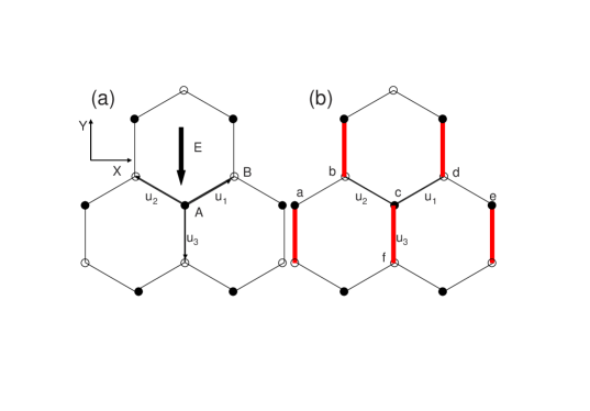
Figure 1: (a) Planar honeycomb lattice with electric field along Y direction. Black dots are sites of sublattice A and white dots are sites of sublattice B. (b) The effective dimerization bond pattern. The effective hopping constants along the (red) thick bonds are different from those along (black) thin bonds.

The planar honeycomb lattice (Fig.1(a)) consists of two equivalent sublattices A (black dots) and B (white dots). We consider the charged particle hopping between the nearest neighbor sites from different sublattices. In addition, the system under consideration is subject to a time-periodic electric field ${\bf E}(t)={\bf E}_{0}\cos(\omega t)$. The tight-binding Hamiltonian has the form

$$H=\sum_{<i,j>}V(c_{i}^{+}c_{j}+c_{j}^{+}c_{i})+\sum_{i}e{\bf E}(t)\cdot{\bf r}_{i}c_{i}^{+}c_{i},$$ (1)

where $<i,j>$ refers to the nearest neighbor lattice sites, ${\bf r}_{i}$ is the position of site $i$. The probability amplitude $\alpha({\bf r}_{i})$ for a particle at site $i$ of sublattice A (or $\beta({\bf r}_{i})$ at site of sublattice B ) can be calculated by solving the corresponding Schr$\ddot{o}$dinger equation. It is very helpful to make the unitary transformation $\alpha({\bf r}_{i})\rightarrow\alpha({\bf r}_{i})e^{-i{\bf A}(t)\cdot{\bf r}_{i}}$ ($\beta({\bf r}_{i})\rightarrow\beta({\bf r}_{i})e^{i{\bf A}(t)\cdot{\bf r}_{i}}$), where ${\bf A}(t)=\frac{\displaystyle e{\bf E}_{0}a}{\displaystyle\omega}\sin(\omega t)$, with $a$ the lattice constant. The subsequent Fourier transformation leads to

$$\begin{array}[]{l}i\frac{\displaystyle d}{\displaystyle dt}\left(\begin{array}[]{c}\alpha({\bf k})\\ \beta({\bf k})\end{array}\right)\,\par=H({\bf k},t)\left(\begin{array}[]{c}\alpha({\bf k})\\ \beta({\bf k})\end{array}\right)\,,\end{array}$$ (2)

$$\begin{array}[]{l}H=\left(\begin{array}[]{cc}0&V\sum_{j=1,2,3}e^{i(a{\bf k}-{\bf A}(t))\cdot{\bf u}_{j}}\\ V\sum_{j=1,2,3}e^{-i(a{\bf k}-{\bf A}(t))\cdot{\bf u}_{j}}&0\end{array}\right)\end{array}$$ (3)

Due to the Floquet theorem, the quasienergy can be obtained by diagonalizing the time evolution operator $\hat{T}\int_{0}^{T}dte^{-iH({\bf k},t)}$, where $\hat{T}$ refers to time ordering and T is the period of the AC field . We first consider the case of electric field along Y direction. In the high frequency limit $V/\omega<<1$, we can obtain the following analytical result for quasienergy spectrum

$$\varepsilon=\pm V\sqrt{A^{2}+4B^{2}(\cos\frac{\displaystyle\sqrt{3}}{\displaystyle 2}k_{x}a)^{2}+4AB\cos\frac{\displaystyle\sqrt{3}}{\displaystyle 2}k_{x}a\cos\frac{\displaystyle 3}{\displaystyle 2}k_{y}a},$$ (4)

where $A=J_{0}(eE_{0}a/\omega)$ and $B=J_{0}(eE_{0}a/2\omega)$, $J_{0}$ is the zero-th order Bessel function. When $E_{0}\rightarrow 0$, $A,B\rightarrow 1$, we reproduce the results for energy spectrum of a system with honeycomb lattice without AC electric field.

Quantum phase transition The conduction band and valence band may form conically shaped valleys that touch at some specific points (called conical points or Dirac points). These Dirac points are determined as $k_{y}a=2\pi/3$, $\cos(\frac{\displaystyle\sqrt{3}}{\displaystyle 2}k_{x}a)=A/2B$. It is clear that there is no solution, when $|A|>2|B|$. In this situation, an energy gap is generated. In Fig. 2 (red solid curve) we show $|A|/2|B|=|J_{0}(x)/2J_{0}(x/2)|$ versus $x=eE_{0}a/\omega$.

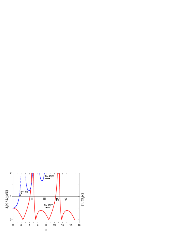
Figure 2: Red solid curve: $|A|/2|B|=|J_{0}(x)/2J_{0}(x/2)|$ versus x; Blue dotted curve: $|1/2J_{0}(x)|$ versus x.

From Fig. 2 it can be seen that gap opening happens in the regimes (for $eE_{0}a/\omega$) II=[4.1, 5.1], IV=[10.3, 11.3],…. Figures 3(a)-(f) (corresponding to regimes I to V) show the quasienergy spectra around the minimum of conduction band/maximun of valence band for different values of $eE_{0}a/\omega$, which are obtained by exact numerical calculation based on Eqs. (2) and (3).

Figure 3: Quasienergy spectra for $eE_{0}a/\omega$=3.5 (in regime I), $eE_{0}a/\omega$=4.60 (in regime II), $eE_{0}a/\omega$=4.81 (band collapse condition), $eE_{0}a/\omega$=5.52 (in regime III), $eE_{0}a/\omega$=10.8 (in regime IV), and $eE_{0}a/\omega$=12.5 (in regime V), are obtained by exact numerical calculation. $V/\omega=0.02$.

We can see from figure 3 that as $eE_{0}a/\omega$ increases, the system undergoes a series of phases corresponding to the regimes I-V, i.e., gapless phase (regime I) $\rightarrow$ gapped phase (regime II) $\rightarrow$ gapless phase (regime III) $\rightarrow$ gapped phase (regime IV) $\rightarrow$ gapless phase (regime V). The gap opening introduces a new energy scale and may also lead to the generation of an effective mass as seen in Figs. 3(b) and (e), since the quasienergy spectrum near the bottom of conduction band is parabolic. We find the gap and the effective mass are proportional to $D=(|A|-2|B|)\theta(|A|-2|B|)$. Thus D is the order parameter, which is zero in the massless phases and nonzero in the gapped phases. As one can see from figure 3, with tuning AC field, the Dirac points may disappear in the gapped phase, or change from discrete points to a line as shown in Fig. 3(d). Near $\varepsilon=0$, the density of quasienergy states $D(\varepsilon)$ is zero for gapped phases, $D(\varepsilon)\sim|\varepsilon|$ near discrete Dirac points, and $D(\varepsilon)\sim$ constant near the line. According to the generalized Kubo-Greenwood formula for time-dependent systemshi , the conductivity depends on the density of quasienergy states. Therefore by simply tuning the strength of external AC field, we can realize the transitions from “metal” phase to “semimetal” phase and to “semiconductor”/“insulator” phase.

Band collapse A typical character of Fig. 2 is that $|A|/2|B|$ is divergent at $eE_{0}a/\omega=4.81,11.0,...$. By checking Eq. (4), it is easy to see that band collapse happens and a gap opens under this condition B=0 or $J_{0}(eE_{0}a/2\omega)=0$. Figure 3(c) shows the quasienergy spectrum for $eE_{0}a/\omega=4.81$, twice of 2.405, the first zero point of $J_{0}$. As expected, we see the flat conduction and valence bands, which are drastically different from the remaining figures of Fig. 3, and the case without an AC field. Moreover we see a gap between conduction and valence bands opens. From eq. (4), one can also see that the quasienergy band collapses in the Y direction, when A=0, i.e., $eE_{0}a/\omega=2.405$,….

Time-dependent dynamics The collapse of quasienergy spectrum implies dynamical localization. To verify this picture, we calculate the time evolution of a particle initially at the origin. In our calculation, the system size is 101 $\times$ 101, time step=0.02 (in unit of $1/\omega$), and the hopping constant is $V/\omega=0.02$ as that in the calculation of quasienergy. In the long time regime, the mean square displacement of the particle shows the time-dependent behavior as $t^{\alpha}$. In figure 4(a) we show the time dependence of the mean square displacement. We can see that when the system is away from band collapse condition ($eE_{0}a/\omega=4.81$), $\alpha=2$, the dynamics is a typical ballistic motion. Under the band collapse condition, the mean quare displacement is finite ($<1$) for all the time, i.e., $\alpha=0$, indicating the dynamical localization of the particle due to the presence of an AC field. In Fig. 4(b), we show the time dependence of the mean square displacement in the X and Y directions for $eE_{0}a/\omega=2.405$, under which the quasienergy spectrum is flat in the Y direction. It is clear that the particle is localized in the Y direction ($<m^{2}_{y}><0.18$), indicating a dimension reduction from 2D to 1D.

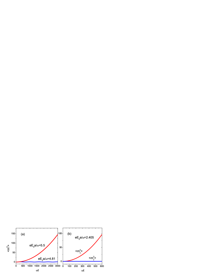
Figure 4: (a) Time dependence of the mean square-displacement for $eE_{0}a/\omega=4.81$ and $eE_{0}a/\omega=5.50$; (b)Time dependence of the mean square-displacement in the X and Y directions for $eE_{0}a/\omega=2.405$.

Renormalization of velocity of “light” For system in the gapless phases, we may obtain the velocity of “light” by expanding the quasienergy spectrum around Dirac points

$$\begin{array}[]{l}v_{x}=2Bt\sqrt{3}\sin(\frac{\displaystyle\sqrt{3}}{\displaystyle 2}\bar{k}_{x}a)\\ v_{y}=6Bt\cos(\frac{\displaystyle\sqrt{3}}{\displaystyle 2}\bar{k}_{x}a),\end{array}$$ (5)

where $\{\bar{k}_{x}a,\bar{k}_{y}a\}$ refer to the Dirac points. We can see that the velocity of “light” can be tuned by the amplitude and frequency of external electric field. From Fig. 5(a), one can see that the velocity of “light” for $eE_{0}a/\omega=3.5$ reduces to $\sim\frac{\displaystyle 1}{\displaystyle 3}$ of that without external electric field. The external field may also lead to the anisotropy of velocity of “light”, see figure 5(b) and Eq. (5). An extremal example is that the velocity in one direction is finite, while in the other direction becomes zero under the condition A=0, i.e. $\cos(\frac{\displaystyle\sqrt{3}}{\displaystyle 2}\bar{k}_{x}a)=0$, as shown in Fig. 3(d). The tunability of velocity of “light” gives us more opportunities to explore relativistic effects in electronic systems or optical lattices.

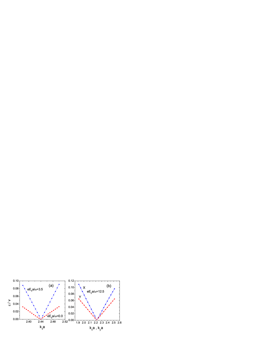
Figure 5: Renormalization of the velocity of “light”. (a) Quasienergy spectrum for $eE_{0}a/\omega$=0.0 and 3.5. (b) Anisotropy of velocity of “light”. Quasienergy spectrum for $eE_{0}a/\omega=12.5$. For the purpose of comparison, we have shifted the coordinates of Dirac points.

Dependence on the direction of electric fields The quasienergy spectrum is dependent on the direction of electric field. For the case of an electric field along X direction, the quasienergy spectrum still takes the form of Eq. (4) with A=1 and $B=J_{0}(\frac{\displaystyle\sqrt{3}}{\displaystyle 2}eE_{0}a/\omega)$. In this case the condition for the existence of Dirac points is $|2J_{0}(\frac{\displaystyle\sqrt{3}}{\displaystyle 2}eE_{0}a/\omega)|\geqslant 1$. From Figure 2(b) (dotted blue curve), we see that when $\frac{\displaystyle\sqrt{3}}{\displaystyle 2}eE_{0}a/\omega>1.52$ or $eE_{0}a/\omega>1.76$, a gap always opens, which is quite contrast to the case with electric field along Y direction discussed above. The band collapse appears under the new condition $J_{0}(\frac{\displaystyle\sqrt{3}}{\displaystyle 2}eE_{0}a/\omega)=0$.

In the more general situation, the quasienergy spectrum has the form $\varepsilon=\pm V\sqrt{|\sum_{j}a_{j}e^{-ia{\bf k}\cdot{\bf u}_{j}}|^{2}}$, where $a_{j}=J_{0}(ea{\bf E}_{0}\cdot{\bf u}_{j}/\omega)$. The general condition for the existence of Dirac points or the gapless phase is that $|a_{j}|$ can form a triangle, or $|a_{i}|+|a_{j}|\geqslant|a_{k}|,\{i,j,k\}=\{1,2,3\}$. The conditions for the band collapse/dynamical localization become $a_{i}=a_{j}=0,i,j\in\{1,2,3\}$. These conditions are two equations with two variables, which can be solved in general situation.

Now we give a simple picture of the phenomena we have found. For an electric filed ${\bf E}(t)$ in arbitrary direction, the projection of this field in three directions along the bond (i.e., directions ${\bf u}_{i},i=1,2,3$ (see figure 1)) is $E_{i}$. Then the effective hopping constants along the bonds ${\bf u}_{i}$ are $V^{eff}_{i}=VJ_{0}(eE_{i}a/\omega)$. Thus we may map our system to a system with honeycomb lattice and effective hopping constants $V^{eff}_{i}$ along bond ${\bf u}_{i}$. The dynamical localization phenomena we have found are quite clear in this picture. In fact, for the case ${\bf E}//Y$ and $eE_{0}a/\omega=4.81$, $V^{eff}_{1}=V^{eff}_{2}=0$, the particle initially staying at site c can only oscillate between site c and site f (see Fig. 1(b)). It is the dynamical localization behavior shown in Fig. 4(a). For the situation $eE_{0}a/\omega=2.405$, $V^{eff}_{3}=0$, the particle can only move through the path “abcde” shown in Fig.1(b), which is the dynamical localization in the Y direction show in Fig. 4(b). The occurrence of band gap and effective mass is also a consequence of the “bond ordering”, the dimerization pattern (see Fig. 1(b)). In the continuum limit, the fluctuation of hopping constant maps to axial vector potential jackiw . It is different from the honeycomb lattice with “Kekule pattern”, in which the fluctuation of hopping constant maps to the complex-valued Higgs field in the continuum limit. In that case the opening of energy gap is related to the spontaneous breaking of an effective axial U(1) symmetry chamon , and was proposed for the split of zero-energy Landau levels in graphene in the presence of magnetic field hatsugai . By tuning the external electric field, one may effectively obtain different bond patterns.

Realization in optical lattices The honeycomb optical lattice can be realized in experiment oplhoney by using three pairs of laser beams with co-planar propagating wavevectors $\pm{\bf q}_{i},i=1,2,3$. The magnitude of the three pairs of wavevectors are the same and their directions form the angle of 120 degree with each other. The optical potential has the form

$$U=\sum_{i}U_{i}=U_{0}\sum_{i}\cos({\bf p}_{i}\cdot{\bf r}),$$ (6)

where ${\bf p}_{1}={\bf q}_{2}-{\bf q}_{3}$, ${\bf p}_{2}={\bf q}_{3}-{\bf q}_{1}$, and ${\bf p}_{3}={\bf q}_{1}-{\bf q}_{2}$. $U_{0}$ depends on the detuning between laser frequency and atomic transition frequency, and the resonant Rabi frequency proportional to the the quare root of laser intensity opldyn . Thus $U_{0}$ can be tuned quite easily in experiments. For sufficient large detuning, we may neglect spontaneous scattering and the high frequency condition $U_{0}/\omega<<1$ can also be easily met. To simulate the electronic force in electronic system, we may let the coordinate of the mirror in each direction ${\bf p}_{i}$ , reflecting the incoming traveling light wave, oscillate around its average with $d_{i}\cos(\omega t)$. Its effect is to replace the atomic effective potential $U_{0}\cos({\bf p}_{i}\cdot{\bf r})$ with $U_{0}\cos({\bf p}_{i}\cdot{\bf r}-d_{i}\cos(\omega t))$. In the moving frame of the potential, the atoms feel an effective force proportional to $d_{i}\cos(\omega t)$, which is proportional to the electrical field component in the ${\bf p}_{i}$ direction.

In summary, we have studied the quasienergy spectra and the related dynamics of a particle in honeycomb lattices driven by an AC field. By tuning the amplitude, frequency, and direction of the electric field, we can obtain quite rich phases, including gapped and gapless phases. Moreover we may tune the velocity of the “light”, and realize band collapse and the dimension reduction from 2D to 1D and 0D (dynamical localization in one direction and two directions). In the current paper, we have focused on the high frequency regime, i.e. $V/\omega<<1$. In graphene with V around 2.8eV and the lattice constant $a$ 1.4 Å, our predictions may not be verified easily. However, they should be quite easy to be observed in optical lattices. We leave the low frequency regime for future study.

Acknowledgments This work was partially supported by the National Science Foundation of China under Grants Nos. 10574017, 10744004 and 10604010.

References

- (1)
- (2) P. R. Wallace, Phys. Rev. 71, 622 (1947).
- (3) A.K.Geim and K.S. Novoselov, Nature Materials 6, 183 (2007); A. H. Castro Neto, F. Guinea, N. M. R. Peres, K. S. Novoselov, and A. K. Geim, arXiv:0709.1163.
- (4) K.S. Novoselov, A.K. Geim, S.V. Morozov, D. Jiang, M.I. Katsnelson, I.V. Grigorieva, S.V. Dubonos, and A.A. Firsov, Nature 438, 197 (2005); Y. Zhang, Y.-W. Tan, H.L. Stormer, and P. Kim, Nature 438, 201 (2005).
- (5) G. Grynberg, B. Lounis, P. Verkerk, J.-Y. Courtois, and C. Salomon, Phys. Rev. Lett. 70, 2249 (1993).
- (6) L. B. Shao, S.-L. Zhu, L. Sheng, D. Y. Xing, and Z. D. Wang, arXiv:0804.1850.
- (7) C. Wu, D. Bergman, L. Balents and S. D. Sarma, Phys. Rev. Lett. 99, 070401 (2007); C. Wu and S. D. Sarma, arXiv:0712.4284.
- (8) L. H. Haddad and L. D. Carr, arXiv:0803.3039.
- (9) F. Grossmann, T. Dittrich, P. Jung, and P. Hänggi, Phys. Rev. Lett. 67, 516 (1991).
- (10) K. W. Madison, M. C. Fischer, R. B. Diener, Qian Niu, and M. G. Raizen Phys. Rev. Lett. 81, 5093 (1998).
- (11) M. Holthaus, Phys. Rev. Lett. 69, 351 (1992).
- (12) D. H. Dunlap and V. M. Kenkre, Phys. Rev. B 34, 3625 (1986). X.-G. Zhao, Phys. Lett. A 155, 299 (1991); 167, 291 (1992). B. J. Keay, S. Zeuner, S. J. Allen, Jr., K. D. Maranowski, A. C. Gossard, U. Bhattacharya, and M. J. W. Rodwell, Phys. Rev. Lett. 75, 4102 (1995).
- (13) Maxim G. Vavilov, Vinay Ambegaokar, and Igor L. Aleiner, Phys. Rev. B 63, 195313 (2001); M. G. Vavilov, L. DiCarlo, and C. M. Marcus, Phys. Rev. B 71, 241309 (2005).
- (14) Wanyuan Xie, Hui Pan, Weidong Chu, Wei Zhang, and Suqing Duan, arXiv: 0801.3515.
- (15) Junren Shi and X.C. Xie, Phys. Rev. Lett. 91, 086801 (2003).
- (16) R. Jackiw and S.-Y. Pi, Phys. Rev. Lett. 98, 266402 (2007); C. Chamon, C.-Y. Hou, R. Jackiw, C. Mudry, S.-Y. Pi, and A. P. Schnyder, Phys. Rev. Lett. 100, 110405 (2008).
- (17) C.-Y. Hou, C. Chamon and C. Mudry, Phys. Rev. Lett. 98, 186809 (2007).
- (18) Y. Hatsugai, T. Fukui and H. Aoki, arXiv: 0804.4762.
- (19) R. Graham, M. Schlautmann, and P. Zoller, Phys. Rev. A 45, R19 (1992).
- (20) Q. Niu, X.-G. Zhao, G. A. Georgakis, and M. G. Raizen, Phys. Rev. Lett. 76, 4504 (1996).