,

Tomography of many-body weak values: Mach-Zehnder interferometry

Abstract

We propose and study a weak value (WV) protocol in the context of a solid state setup, specifically, an electronic Mach-Zehnder interferometer. This is the first specific proposal to measure both the real and imaginary part (i.e., complete tomography) of a WV. We also analyze the manifestation of many-body physics in the WV to be measured, including finite temperature and shot-noise-like contributions.

The problem of non-invasive measurement of a quantum system is interesting both from the view point of foundations of quantum mechanics and possible applications (e.g. quantum computation). As opposed to the standard strong measurement procedure described by the projection postulate Neuman , weak measurement of an observable, while weakly disturbing the system, provides only partial information on the state of the latter. Normally the outcome of a weak measurement of an observable is its expectation value, which is the weighted average of the eigenvalues of this observable. Major step in formulating alternatives to standard measurement procedure was the proposal of a weak value protocol Aharonov , consisting of a weak measurement (of $\hat{A}$), followed by a strong one (of $\hat{B}$). The outcome of the first is conditional on the result of the second (post-selection). Specifically, if the system is prepared (preselected) in the state $\left|\chi_{i}\right\rangle$, and is postselected in the state $\left|\chi_{f}\right\rangle$, the weak value of the operator $\hat{A}$ is

$${}_{\chi_{f}}\left\langle A\right\rangle_{\chi_{i}}=\frac{\langle\chi_{f}|\hat{A}|\chi_{i}\rangle}{\langle\chi_{f}|\chi_{i}\rangle}=\frac{\langle\chi_{i}|\Pi_{\chi_{f}}\hat{A}|\chi_{i}\rangle}{\langle\chi_{i}|\Pi_{\chi_{f}}|\chi_{i}\rangle},$$ (1)

where $\Pi_{\chi_{f}}=\left|\chi_{f}\right\rangle\left\langle\chi_{f}\right|$ is a projection operator.

In general, the weak value is a complex number and (as opposed to a projective expectation value) its real part can be out of the range of the eigenvalues of $\hat{A}$. In order to obtain non-trivial weak values (e.g., outside the range of the eigenvalues of $\hat{A}$; complex; negative when $\hat{A}$ is positive definite), the preselected state should not be an eigenstate of the measured operator, and $[\hat{A},\hat{B}]\neq 0$.

WV may allow us to explore some fundamental aspects of quantum measurement, including access to simultaneous measurement of non-commuting variables Hongduo:2007aa ; Jordan:2005aa ; dephasing and phase recovery Neder:2007a ; correlation between measurements Sukhorukov:2007aa ; and even new horizons in metrology Aharonov ; Hosten:2008 . While some aspects of WVs have been demonstrated in optics based setups Pryde:2005 , the implementation of weak values in the context of solid state physics is very new Romito:2008 ; Williams:2007 .

Weak values are not just an artifact of a convoluted definition, but indeed do emerge as the outcome of weak measurement of a pre- and post-selected states. Microscopically we consider the coupling of a system to a detector with a Hamiltonian $H=H_{\textrm{S}}+H_{\textrm{D}}+H_{\textrm{int}}$. The interaction Hamiltonian is $H_{\textrm{int}}=\lambda g(t)\hat{p}\hat{A}$. Here $\hat{p}$ is the momentum canonically conjugate to the position of the detector’s pointer, $\hat{q}$, and $\lambda g(t)$ ($\lambda\ll 1$) is a time dependent coupling constant foot1 . Following the weak measurement and the post-selection steps, the expectation value of the coordinate of the pointer (initially equal to $q_{0}$) is given by $\langle\hat{q}\rangle=q_{0}-\lambda\operatorname{Re}[_{\psi}\langle A\rangle_{\phi}]$, i.e., the shift in the pointer is proportional to the real part of the WV. Under more general conditions (i.e., $\hat{p}$, $\hat{q}$ are not canonically conjugated)the imaginary part of the WV may be meaningful too Steinberg:1995 . An experimental procedure which will provide for a full ”tomography” of (both the real and imaginary parts of) the weak value remains a challenge.

Here we report the first systematic study of complex WVs in the context of many electron solid state system, proposing an experimental procedure which will provide for the full “tomography” of (both the real and imaginary part of) WVs. Employing building blocks which are accessible within current technology Ji:2003 , our proposed protocol and the ensuing predictions are amenable to experimental test. In particular, addressing a “system” and a “detector” which are represented by an electronic Mach-Zehnder interferometer (MZI) Ji:2003 (Fig. 1), (i) We propose how to retrieve both the real and the imaginary parts; (ii) We show that the introduction of both a non-pure state and finite temperature ($T$) modify the WV and reduce the visibility of Aharonov-Bohm (AB) oscillations; (iii) We show how many-body effects lead to reduction of the weak value’s visibility, as a function of voltage bias. In particular $\mbox{\rm Im}[{}_{\chi_{f}}\left\langle A\right\rangle_{\chi_{i}}]$ maintains its single particle value while $\mbox{\rm Re}[{}_{\chi_{f}}\left\langle A\right\rangle_{\chi_{i}}]$ is modified by an excess (non-equilibrium) noise and thermal noise terms; (iv) We show that for the system at hand the WV is related to a system-detector current-current cross correlator foot2 .

The chiral leads of the MZI are realized by the edge states of an integer quantum Hall setup. Throughout this analysis we will consider non-interacting single edge channels ($\nu=1$) foot6 . We do account here for the system-detector interaction and for the inherent many-fermion physics.

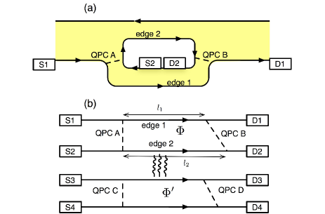
Figure 1: (a) Electronic MZI represented by edge states (full lines) in a Hall bar. Inter-edge tunneling (dashed lines) takes place at the quantum point contacts. (b) Scheme of a double electronic MZI. Electrons on edge states 2 and 3 interact via Coulomb interaction.

Our model Hamiltonian for the system (S) and the detector (D) is Chalker:2007

$$H_{S}=-iv\sum_{m=1}^{2}\int dx:\psi^{{\dagger}}_{m}(x)\partial_{x}\psi_{m}(x):$$

$$+\Gamma_{a}\psi^{{\dagger}}_{1}(0)\psi_{2}(0)+\Gamma_{b}\psi^{{\dagger}}_{1}(l_{1})\psi_{2}(l_{2})+H.c.\,,$$ (2)

$$H_{D}=-iv\sum_{m=3}^{4}\int dx:\psi^{{\dagger}}_{m}(x)\partial_{x}\psi_{m}(x):$$

$$+\Gamma_{c}\psi^{{\dagger}}_{3}(0)\psi_{4}(0)+\Gamma_{d}\psi^{{\dagger}}_{3}(l_{3})\psi_{4}(l_{4})+H.c.$$ (3)

Here $\psi^{{\dagger}}_{m}(x)=\frac{1}{\sqrt{L}}\sum_{k=-\infty}^{\infty}e^{ikx}d^{{\dagger}}_{km}$ is the creation operator at point $x$ on arm $m$ (the system’s length, $L$, is assumed to be much larger than any other length scale in the problem). The $\Gamma$’s are inter-edge tunneling amplitudes, normal ordering is with respect to the vacuum (states are occupied for $k\leq 0$ and empty otherwise), $v$ is the edge velocity and $\hbar=1$. We assume a weak capacitive interaction between the system and the detector:

$$H_{\textrm{int}}=\int dx\,dye^{2}U(x,y):\psi^{{\dagger}}_{2}(x)\psi_{2}(x)::\psi^{{\dagger}}_{3}(y)\psi_{3}(y):\,,$$

where the support of $U(x,y)$ is $0<x,y<\min_{m}{(l_{m})}$. Without loss of generality we assume that sources $S1$ and $S3$ are voltage biased ($V$ and $V_{3}$), and use the current at $D4$ as the weak measurement’s pointer.

$H_{S}$ is readily diagonalized. In the Heisenberg representation the system’s $\psi$ operators are

$$\psi_{m}(x,t)=\frac{1}{\sqrt{L}}\sum_{k}e^{ik(x-vt)}\left\{\begin{array}[]{ll}a_{km},&\hbox{$x<0;$}\\ b_{km},&\hbox{$0<x<l_{m};$}\\ c_{km},&\hbox{$l_{m}<x.$}\\ \end{array}\right.$$ (7)

where $m=1,2$ and $\mathbf{b}_{k}=\mathcal{S}_{A}\mathbf{a}_{k}$, $\mathbf{c}_{k}=\mathcal{S}_{B}\mathbf{b}_{k}$ with scattering matrices $\mathcal{S}_{i}=\left(\begin{array}[]{cc}r_{i}&t_{i}\\ -t_{i}^{*}&r_{i}\\ \end{array}\right)$ ($i=a,b$) and, for equal arm lengths, $r_{i}=[(2v)^{2}-|\Gamma_{i}|^{2}]/[(2v)^{2}+|\Gamma_{i}|^{2}]$, $t_{i}=4iv\Gamma_{i}/[(2v)^{2}+|\Gamma_{i}|^{2}]$. The effect of the system’s AB phase and unequal arm’s lengths can be absorbed into $\tilde{\Gamma}_{A}\equiv\Gamma_{A}e^{i\tilde{\phi}/2}$, $\Gamma_{B}\equiv\Gamma_{B}e^{-i\tilde{\phi}/2}$. Here $\tilde{\phi}$ includes the contributions of both the AB flux, $\Phi$, and the orbital phase: $\tilde{\phi}\equiv\phi+k(l_{2}-l_{1})$, $\phi\equiv 2\pi\frac{\Phi}{\Phi_{0}}$ ($\Gamma_{A},\Gamma_{B}>0$). A similar expression is available for $H_{D}$ as well.

As a first step we consider the injection of a single particle (in the scattering state $k$) into the system foot3 (e.g., at the source S1). The preselected state is then $\left|S_{1}\right\rangle=a_{k1}^{{\dagger}}\left|0\right\rangle$. The post-selected state is $\left|D_{2}\right\rangle=c_{k2}^{{\dagger}}\left|0\right\rangle$ (detection at D2). By definition (1) the WV of the charge at the intermediate segment of arm $i$ is ${}_{D2}\langle\hat{Q}_{i}\rangle_{S1}^{\textrm{SP}}/e=\frac{\langle c_{k2}b^{{\dagger}}_{ki}b_{ki}a^{{\dagger}}_{k1}\rangle}{\langle c_{k2}a^{{\dagger}}_{k1}\rangle}$, yielding ${}_{D2}\langle\hat{Q}_{2}\rangle_{S1}^{\textrm{SP}}/e=\frac{t_{A}^{*}r_{B}}{t_{A}^{*}r_{B}+e^{i\tilde{\phi}}r_{A}t_{B}^{*}}$ (pure state). This quantity may assume complex values depending on the choice of parameters (transmission and reflection amplitudes and $\Phi$). In particular, its real part may be larger than $1$ or even negative, clearly outside the allowed range of the number operator expectation value. But, as expected, ${}_{D2}\langle Q_{1}\rangle_{S1}^{\textrm{SP}}+_{D2}\langle Q_{2}\rangle_{S1}^{\textrm{SP}}=e$. The individual weak values are $\Phi_{0}$ periodic with the flux.

In a more general case, when the system is initially not in a pure state (e.g., finite temperature, entanglement, etc.), eq. (1) is not applicable, and we have to rewrite it in terms of the density matrix, $\rho$, of the initial state, yielding Romito:2008 :

$${}_{\chi_{f}}\left\langle A\right\rangle_{\chi_{i}}\equiv\frac{\mathop{Tr}(\Pi_{\chi_{f}}\hat{A}\rho)}{\mathop{Tr}(\Pi_{\chi_{f}}\rho)}=\frac{\langle\chi_{f}|\hat{A}\rho|\chi_{f}\rangle}{\langle\chi_{f}|\rho|\chi_{f}\rangle}\,.$$

For example assume that a voltage bias $V$ is applied to the source S1, which is held at temperature $T$. Then $\rho=1/L\sum_{k}[f(vk-eV)-f(vk)]a_{k1}^{{\dagger}}a_{k1}$, with $f(x)$ the Fermi-Dirac distribution at zero voltage bias, and

$${}_{D2}\langle Q_{2}\rangle_{S1}^{\textrm{SP}}=\frac{t_{A}^{*}r_{B}(t_{A}r_{B}+K(V,T)e^{-i\varphi}r_{A}t_{B})}{|r_{A}t_{B}|^{2}+|t_{A}r_{B}|^{2}+2K(V,T)\mbox{\rm{Re}}[e^{i\varphi}r_{A}t_{B}^{*}t_{A}r_{B}]}\,,$$ (8)

where $\varphi=eV\Delta l/(2v)+\phi$, $K(V,T)\equiv\frac{2\pi k_{B}T\sin(eV\Delta l/(2v))}{eV\sinh(\pi k_{B}T\Delta l/v)}$ and $\Delta l=l_{2}-l_{1}$. We observe that the broadening of the energy and non-pure nature of the initial state lead to the suppression of the interference term, which in turn leads to the suppression of the imaginary part of the WV and reduces the real part to a ”standard” value lying in the interval $[0,1]$.

We next study the generalization of this protocol to a many-body (albeit non-interacting) system. The preselected state is given by the stationary voltage biased ($V$) non-equilibrium state of the system. Post-selection will be defined by the detection of one electron at the drain D2, i.e. within $[x-\varepsilon,x+\varepsilon]$, $\epsilon\rightarrow 0$ around $x>l_{1},l_{2}$. The projection operator for this state is $:\psi_{2}^{{\dagger}}(x)\psi_{2}(x):$. For a system with linear dispersion relation, the current operator is $\hat{I}_{2}(x,t)=ev:\psi_{2}^{{\dagger}}(x,t)\psi_{2}(x,t):$; it follows that we can employ $\hat{I}_{2}/(ev)$ as a projection operator for the post-selection. We consider the WV of charge (or current) at the intermediate segment of arm $2$. It is given by the operator $\hat{Q}_{2}(x_{0})=ev\int_{-\tau/2}^{\tau/2}dt:\psi^{{\dagger}}_{2}(x_{0},t)\psi_{2}(x_{0},t):$, where $\tau$ is an infrared cut-off, $\tau\gg\frac{L}{v}$, and $0<x_{0}<l_{2}$. Such an operator can be measured e.g. by adiabatically switching on (off) the coupling to the measurement device at $t<0$ ($t>0$) foot4 . From (1), and employing $\langle a^{{\dagger}}_{ki}a_{ki}\rangle=f(vk-\mu_{i})$ with $\mu_{1}=eV,~{}\mu_{2}=0$, we obtain foot5 :

$${}_{D2}\left\langle Q_{2}\right\rangle_{S1}^{\textrm{MB}}=\frac{\langle I_{2}(x,0)Q_{2}(x_{0})\rangle}{\langle I_{2}(x,0)\rangle}=\frac{e}{1/L\sum_{k}(f_{eV}-f_{0})\mathcal{A}_{11}}\Bigl{[}\sum_{i,j=1,2}\frac{1}{L}\sum_{k}\mathcal{A}_{ij}\mathcal{B}_{ji}f_{\mu_{i}}(1-f_{\mu_{j}})\Bigr{]}+v\tau\sum_{k}(f_{eV}-f_{0})\mathcal{B}_{11}\Bigr{]}\,.$$ (9)

Here $\mathcal{A}_{ij}\equiv(\mathcal{S}_{A}^{{\dagger}}\mathcal{S}_{B}^{{\dagger}})_{i2}(\mathcal{S}_{B}\mathcal{S}_{A})_{2j}$, $\mathcal{B}_{ij}\equiv(\mathcal{S}_{A}^{{\dagger}})_{i2}(\mathcal{S}_{A})_{2j}$ and $f_{\mu}$ stands for the Fermi distribution function $f(vk-\mu)$. The summation over $k$ is replaced by energy integrals, $1/L\sum_{k}\rightarrow 1/(2\pi v)\int dE$. At zero temperature the WV (9) is:

$${}_{D2}\left\langle Q_{2}\right\rangle_{S1}^{\textrm{MB}}={}_{D2}\left\langle Q_{2}\right\rangle_{S1}^{\textrm{SP}}+(N-1)\langle Q_{2}\rangle\,\,\,\,(T=0)\,.$$ (10)

Here $N=\frac{eV\tau}{2\pi}$ is the number of electrons injected into the MZI during the measurement time. The first term on the r.h.s is the single particle WV (8). The second term is proportional to the single particle expectation value of $\hat{Q}_{2}=|t_{A}|^{2}$. This can be interpreted in the following way: the post-selection enforces a detection of one electron at point $x$ at time $t$. The correlation between $\hat{Q}_{2}$ and a post-selection yields the first term. All other electrons which are injected into the system during the measurement are not constrained by the postselection and therefore give rise to an additional contribution to ${}_{D2}\left\langle Q_{2}\right\rangle_{S1}^{\textrm{MB}}$.

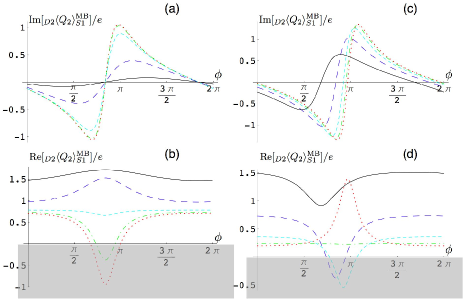
Figure 2: Real and Imaginary part of the many-body WV as a function of the Aharanov-Bohm phase. Panels (a), (b) correspond to different plots for different values of temperature: $T\Delta/l/(\hbar v)=$$0$ (dotted), $0.05$ (dash-dotted), $0.15$ (dashed), $0.5$ (long-dashed), $1.2$ (full). $V=5\mu e$V. Panels (c), (d) correspond to different plots for different voltage biases: $V\Delta l/(\hbar v)=$$0.2$ (dotted), $0.3$ (dash-dotted), $0.5$ (dashed), $1$ (long-dashed), $2$ (full). $T=3$mK. In all plots $\hbar v/\Delta l=5\times 10^{-6}e$V, $\tau=2\times 10^{-10}$ $s$, $t_{A}=r_{A}=1/\sqrt{2}$, $t_{B}=\sqrt{2}r_{B}=\sqrt{2}/\sqrt{3}$. The range for which $\mbox{\rm{Re}}[_{D2}\langle Q_{2}\rangle_{S1}^{\textrm{SP}}]$ is beyond the interval of standard (strong) values is shadowed.

Consider now a finite temperature. Using $\frac{1}{L}\sum_{k}f_{i}(k)(1-f_{i}(k))\simeq-k_{B}T\int\frac{dE}{2\pi v}\frac{\partial f}{\partial E}$ we can write the weak value as

$$\frac{{}_{D2}\left\langle Q_{2}\right\rangle_{S1}^{\textrm{MB}}}{e} = \mbox{\rm{Re}}\left[\frac{F(V,T)\left(|r_{B}r_{A}t_{A}|^{2}-|t_{B}t_{A}r_{A}|^{2}\right)+\left(|r_{A}|^{2}-|t_{A}|^{2}\right)\bar{K}(V,T)e^{i\varphi}r_{A}t_{A}r_{B}t_{B}^{*}}{|r_{A}t_{B}|^{2}+|t_{A}r_{B}|^{2}+2K(V,T)\mbox{\rm{Re}}(e^{i\varphi}t_{A}r_{B}r_{A}t_{B}^{*})}+|t_{A}|^{2}\right]$$ (11)

$$+i\mbox{\rm{Im}}[\frac{{}_{D2}\left\langle Q_{2}\right\rangle_{S1}^{\textrm{SP}}}{e}]+\frac{k_{B}T|r_{B}|^{2}}{eV\left(|r_{A}t_{B}|^{2}+|t_{A}r_{B}|^{2}+2K(V,T)\mbox{\rm{Re}}(e^{i\varphi}t_{A}r_{B}r_{A}t_{B}^{*})\right)}+\langle Q_{2}\rangle(N-1).$$

Here $F(V,T)=\coth[eV/(2k_{B}T)]-2k_{B}T/(eV)$, $K(V,T)$ is given by Eq. (8), and Chung:2005 $\bar{K}(V,T)=2\pi k_{B}T[\sin(eV\Delta l/2v)\coth(eV/2k_{B}T)-k_{B}T\Delta l/v\cos(eV\Delta l/2v)]/[eV\sinh(\pi k_{B}T\Delta l/v)]$. This is the central result of the letter. The many body weak value in electronic MZI consists of four terms: (i) A term which is related to the real part of the single particle weak value corrected by finite temperature Fermi sea effects; (ii) The imaginary part of the single particle weak value; (iii) A contribution due to thermal fluctuations Martin:1992 ; (iv) Many body “excess noise”. The dependence of the many-body WV on voltage and temperature is presented in Fig. 2. Note the asymmetry between the imaginary and the real parts of the WV: the former coincides with the imaginary part of the single particle weak independently on the voltage bias and temperature. When the temperature is smaller than the voltage bias, $k_{B}T\ll eV$ the many-body VW reduces to the expression in Eq.(10), while at high temperature the third term dominates and thermal fluctuations wash out the SP weak values.

We now describe the measurement procedure leading to the WVs. We should calculate the expectation value of the pointer’s variable, which, in our case, is the time average of the outgoing current in the drain D4. The latter is given by the expectation value of $\hat{I}_{4}(x^{\prime})=1/\tau\int_{-\tau/2}^{\tau/2}dt\,\hat{I}_{4}(x^{\prime},t)$ ($x^{\prime}>l_{4}$), in the detector’s state after postselection. Post-selection is realized by acting on the system’s state with the projection operator $\hat{I}_{2}(x,t)$. Therefore the effective action of the detector after performing the post-selection and tracing over the system’s state is

$$e^{iS_{D}^{(\textrm{eff})}}=\int\mathcal{D}[\bar{\psi}_{1}\psi_{1}]\mathcal{D}[\bar{\psi}_{2}\psi_{2}]\,I_{2}(x,t)e^{iS},$$ (12)

and the effective partition function is $Z_{D}^{(\textrm{eff})}=\int\mathcal{D}[\bar{\psi}_{3}\psi_{3}]\mathcal{D}[\bar{\psi}_{4}\psi_{4}]\,e^{iS_{D}^{(\textrm{eff})}}$. We calculate the expectation value of $\hat{I}_{4}(x^{\prime},t)$ using this effective partition function, which yields $\left\langle\hat{I}_{4}(x^{\prime})\right\rangle=1/Z_{D}^{(\textrm{eff})}\int\mathcal{D}[\bar{\psi}_{3}\psi_{3}]\mathcal{D}[\bar{\psi}_{4}\psi_{4}]\,I_{4}(x^{\prime})e^{iS_{D}^{(\textrm{eff})}}=\left\langle\hat{I}_{4}(x^{\prime})\hat{I}_{2}(x,t)\right\rangle/\left\langle\hat{I}_{2}(x,t)\right\rangle$. Hence, in order to obtain a weak value we consider the correlator $\left\langle I_{2}(t)I_{4}(t^{\prime})\right\rangle$. Since the system is out of equilibrium we employ the Keldysh technique to calculate this correlator. After some algebra we obtain to first order in the interaction

$$\frac{1}{\tau}\int_{t-\tau/2}^{t+\tau/2}dt^{\prime}\,\left\langle I_{2}(t)I_{4}(t^{\prime})\right\rangle=\left\langle I_{2}\right\rangle_{0}\langle I_{4}\rangle_{0}$$ (13)

$$\times\Bigl{(}1+\frac{2\lambda}{e^{2}\tau}\operatorname{Im}\Bigl{\{}(_{D2}\left\langle Q_{2}\right\rangle_{S1}^{\textrm{MB}})(_{D4}\left\langle Q_{2}\right\rangle_{S3}^{\textrm{MB}})\Bigr{\}}\Bigr{)}\,,$$ (14)

where $\lambda=e^{2}\int dx\,dy\,U(x,y)$, and $\left\langle\phantom{i}\right\rangle_{0}$ refers to the $\lambda=0$ expectation value. Indeed , dividing by $\left\langle I_{2}\right\rangle$, we see that the shift in the detector’s current is proportional to the WV (9). Since here the “system” and the “detector” play a symmetric role, the result can be stated in a system-detector symmetric fashion: for weak enough interaction, the current-current correlator is proportional to the product of WV of the respective system and detector operators which appear in $H_{\textrm{int}}$. Notice that varying the Aharonov-Bohm flux in the ”detector” MZI one can explore the real and the imaginary parts of the ”system’s” WV.

The analysis presented here is the first significant step towards a complete characterization of weak values in interacting systems. The visibility of flux sensitive many-body WVs is reduced by both $T$ and $V$: The single particle WV is supplemented by thermal noise and by a voltage dependent many fermion term. This WV tomography and the tuning of the respective noise terms are all amenable to experimental verification.

We acknowledge illuminating discussions with Y. Aharonov, A. Stern, and L. Vaidmann. This work was supported by the Minerva Foundation, US-Israel BSF and the DFG project SPP 1285, and DFG Priority Programme ”Semiconductor Spintronics”.

References

(1)
J. von Neuman,
Mathematische Grusndlagen der Quantemachanik
(Springler-Verlag, Berlin 1932)
(2)
Y. Aharonov, D. Z. Albert, and L. Vaidman,
Phys. Rev. Lett. 60, 1351 (1988); Y. Aharonov and L. Vaidman,
Phys. Rev. A, 41, 11 (1990).
(3)
W. Hongduo and Y. V. Nazarov, cond-mat/0703344 (2007).
(4)
A. Jordan and M. Buttiker, Phys. Rev. Lett. 95,
220401(2005).
(5)
I. Neder, F. Marquardt, M. Heiblum, D. Mahalu, and
V.Umansky,
Nature Phys. 3, 534 (2007);
I. Neder, M. Heiblum, D. Mahalu, and V. Umansky,
Phys. Rev. Lett. 98, 036803 (2007).
(6)
E. Sukhorukov, A. Jordan, S. Gustavsson, R. Leturcq, T. Ihn and
K.Ensslin, Nature Phys. 3, 243 (2007);
A. Di Lorenzo and Y. V. Nazarov, Phys. Rev. Lett. 93,
046601(2004).
(7)
O. Hosten, and P. Kwiat,
Science 319, 787 (2008)
(8)
G. J. Pryde, J. L. O’Brien, A. G. White, T. C. Ralph, and H. M. Wiseman,
Phys. Rev. Lett. 94, 220405 (2005);
A. M. Steinberg,
Phys. Rev. Lett. 74, 2405 (1995);
H. M. Wiseman,
Phys. Rev. A 65, 032111 (2002).
(9)
Alessandro Romito, Yuval Gefen, and Yaroslav M. Blanter,
Phys. Rev. Lett. 100, 056801 (2008).
(10)
N. S. Williams and A. N. Jordan,
Phys. Rev. Lett. 100, 026804 (2008).
(11)
In this example we have assumed that the free Hamiltonians of the
system and the detector vanish and that .
(12)
See e.g., A. M. Steinberg,
Phys. Rev. A 52, 32 (1995);
L. M. Johansen,
Phys. Lett. A 322, 298 (2004);
R. Jozsa,
Phys. Rev. A 76, 044103 (2007);
We have learned of the interesting work of A. Di Lorenzo and J. C. Egues, [arXiv:0801.1814].
(13)
Y. Ji, Y. Chung, D. Sprinzak, M. Heiblum, D. Mahalu and
H. Shtrikman,
Nature 422, 415 (2003);
P. Roulleau, F. Portier, D. C. Glattli, P. Roche, A. Cavanna, G. Faini, U. Gennser, and D.
Mailly,
[arXiv:0704.0746v2];
I. Neder, N. Ofek, Y. Chung, M. Heiblum, D. Mahalu, and V. Umansky,
Nature 448, 333 (2007).
(14)
We believe that a qualitatively similar statement
(concerning a system-detector two operator cross-correlator)
applies to weak value protocols at large.
(15)
While this simplified picture may not account for some aspects of the
problem [dephasing (cf. F. Marquardt and C. Bruder,
Phys. Rev. Lett. 92, 056805 (2004)), ”lobe” structure, etc.],
we find it as a relevant reference model to account
for the weak value physics
(16)
J. T. Chalker, Yuval Gefen, and M. Y. Veillette,
Phys. Rev. B 76, 085320 (2007)
(17)
Note that a single particle MZI can be mapped onto the problem of spin particle.
Indeed, choose the -axis such that and
. Then ,
the scattering matrices rotate the spin in, say, the plane and the AB flux rotate the spin around the -axis.
(18)
allows us to replace the weak
measurement signal taken over a finite segment by an operator defined at a point ().
(19)
This expression is readily generalized to the situation in which bias is applied to
the source Sα, the post-selected electron is detected at Dβ, and the
weakly measured operator is . In this case one has to replace the index
in the definition of by , and in by .
The index in , , and is replaced by
the index .
(20)
V. S. -W. Chung, P. Samuelsson, M. Buttiker,
Phys. Rev. B 72, 125320 (2005).
(21)
Th. Martin, R. Landauer,
Phys. Rev. B 45, 1742 (1992).