On the applicability of bosonization and the Anderson-Yuval methods at the strong-coupling limit of quantum impurity problems

Abstract

The applicability of bosonization and the Anderson-Yuval (AY) approach at strong coupling is investigated by considering two generic impurity models: the interacting resonant-level model and the anisotropic Kondo model. The two methods differ in the renormalization of the conduction-electron density of states (DoS) near the impurity site. Reduction of the DoS, absent in bosonization but accounted for in the AY approach, is shown to be vital in some models yet superfluous in others. The criterion being the stability of the strong-coupling fixed point. Renormalization of the DoS is essential for an unstable fixed point, but superfluous when a decoupled entity with local dynamics is formed. This rule can be used to boost the accuracy of both methods at strong coupling.

—Introduction. Several classic models in condensed-matter physics show logarithmic behavior at high energies, followed by qualitatively different behavior at low energies. Notable examples include the x-ray absorption problem, NozieresDeDominicis69 the Kondo Hamiltonian, Kondo64 the interacting resonant-level model (IRLM), VigmanFinkelstein78 ; Schlottmann82 and different variants of two-level systems (TLS). YuAnderson84 ; VladarZimanyi88 Historically devised to model real impurities in bulk samples, many of these Hamiltonians have recently found new realizations and generalizations in quantum dots and other confined nanostructures.

A distinguished place in the theory of such quantum impurities is reserved to Abelian bosonization bosonization and the Anderson-Yuval (AY) approach, AndersonYuval70 ; AndersonHamann70 which remain among the most powerful and versatile analytical tools in this realm. With numerous applications over the last forty years, it is surprising that the applicability of neither approach has ever been studied systematically for strong couplings. In bosonization, the bare couplings are generally assumed to be weak. Strong static interactions are often included ad hoc in terms of their scattering phase shift. The AY method, which maps the original impurity problem onto an effective Coulomb gas, is presumably nonperturbative in certain couplings. However, it typically fails to reproduce the correct scaling equations even at the next-to-leading order. FowlerZawadowski71 ; Schlottmann82 A reliable extension of these approaches to strong couplings is highly desirable.

The goal of the present paper is to critically test the accuracy of these leading analytic methods away from weak coupling, and to propose an operational extension to strong couplings. To this end, we resort to Wilson’s numerical renormalization group Wilson75 (NRG), and to two generic classes of models as test beds: the IRLM and the anisotropic Kondo model. Our analysis highlights the role of the reduction in the conduction-electron density of states (DoS) near the impurity site, which may hinder the efficiency of other essential couplings (e.g., tunneling in the IRLM). This reduction of the DoS, absent in bosonization but included in the AY approach, proves vital in some models and superfluous in others. It is essential in cases where the strong-coupling fixed point is unstable, but superfluous in models where a decoupled entity with local dynamics is formed at strong coupling. Hence, the accuracy of bosonization and the AY approach can be significantly enhanced by selectively incorporating the DoS renormalization factor to match the case in question.

The reduction of the local conduction-electron DoS is best seen for a simple model where electrons scatter elastically off a point-like impurity ($s$-wave scattering). The renormalized DoS at the impurity site takes the form MezeiZawadowski71

$$\varrho(\omega\approx E_{\rm F})=\varrho_{0}\cos^{2}\delta\;,$$ (1)

where $\varrho_{0}$ is the unperturbed DoS, $E_{\rm F}$ is the Fermi energy, and $\delta$ is the scattering phase shift. Since $\delta\to\pi/2$ for resonant scattering, this implies $\varrho(\omega\approx E_{\rm F})\to 0$. This fact may have a dramatic effect, as exemplified below by the two-channel IRLM. A strong local Coulomb repulsion suppresses the DoS at the vicinity of the impurity, reducing the hopping rate between the impurity and the bands. Since reduction of the DoS is independent of the interaction sign, it equally applies to an alternating potential. The case of a TLS with a single coupling (the commutative model YuAnderson84 ; VladarZimanyi88 ) is qualitatively similar.

One may expect the same to occur in the anisotropic Kondo model or the non-commutative TLS with electron-assisted hopping. For example, consider the single-channel Kondo model (1CKM) with a large $XXZ$ anisotropy: $J_{z}\gg|J_{\perp}|$, with $J_{x}=J_{y}=J_{\perp}$. In the spirit of the AY philosophy, AndersonYuval70 one may first treat the larger coupling $J_{z}$ before incorporating the smaller $J_{\perp}$. In the absence of $J_{\perp}$, a large $J_{z}$ reduces the local DoS at the impurity site independent of the orientation of the impurity spin. Incorporating $J_{\perp}$ at the next step, its efficiency is expected to be hindered by the reduced DoS, to the extent that it diminishes in the limit $J_{z}\to\infty$ [when $\delta\to\pi/2$ and $\varrho(\omega\approx E_{\rm F})\to 0$]. Surprisingly, this is not what we find with the NRG. Rather, spin flips remain governed at large $J_{z}$ by the bare transverse coupling $J_{\perp}$.

To unravel the governing rule, we conduct a detailed comparison between Wilson’s NRG, bosonization, and the AY method, applied separately to the multichannel Kondo and IRLM models. Applicability of the latter two approaches at strong coupling is shown to depend crucially on the stability of the strong-coupling limit. Whenever a decoupled entity with local dynamics is formed (i.e., a stable strong-coupling fixed point is reached), then the DoS renormalization factor is superfluous and bosonization works well. If, however, the strong-coupling limit is unstable, then the DoS renormalization factor is essential and the AY approach works well. The above classification pertains to non-commutative models. For commutative couplings the AY method always applies as one can always reorder the perturbation series.

Prompted by these findings we proceed to re-examine the “intimate relation” between the IRLM and the anisotropic 1CKM. Schlottmann82 Close correspondence is established between the models in case of the single-channel IRLM, but not in the case of multiple screening channels.

—Interacting resonant-level model. In the IRLM, VigmanFinkelstein78 ; Schlottmann82 a 1D electron gas is coupled to a spinless impurity level by two distinct mechanisms: a hopping matrix element $V$ and a short-range Coulomb repulsion $U$. The hopping rate is enhanced for weak repulsion, but is generally suppressed at large $U$ due to a reduction in the conduction-electron overlap integrals between a vacant level and an occupied one GiamarchiNozieres93 ; BordaZawadowski07 (the so-called orthogonality catastrophe Anderson67 ). Consequently, the hopping rate tends to develop a maximum at some intermediate coupling $U$, whose value is pushed toward weak coupling as the number of screening bands $N$ is increased. BordaZawadowski07 This behavior stems from an enhancement of the orthogonality effect with increasing $N$.

Interest in the IRLM has been recently rekindled by a Bethe Ansatz solution of a two-lead version of the model under nonequilibrium conditions. MehtaAndrei06 In its multichannel form, the Hamiltonian reads ${\cal H}={\cal H}_{0}+{\cal H}_{1}+{\cal H}_{2}$, with

$${\cal H}_{0} = \sum_{n=0}^{N-1}\sum_{0<k<2k_{F}}v_{F}(k-k_{F})a^{\dagger}_{kn}a^{\phantom{\dagger}}_{kn}+\epsilon_{d}d^{\dagger}d\;,$$ (2)

$${\cal H}_{1} = U\sum_{n=0}^{N-1}\bigg{(}a^{\dagger}_{n}a^{\phantom{\dagger}}_{n}-\frac{1}{2}\bigg{)}\bigg{(}d^{\dagger}d-\frac{1}{2}\bigg{)}\;,$$ (3)

$${\cal H}_{2} = V\left(d^{\dagger}a^{\phantom{\dagger}}_{0}+a^{{\dagger}}_{0}d\right)\;.$$ (4)

Here, $a^{\dagger}_{kn}$ creates an electron with momentum $k$ in the $n$th band, $d^{\dagger}$ creates an electron on the level, $k_{F}$ and $v_{F}$ are the Fermi momentum and Fermi velocity, respectively, $\epsilon_{d}$ is the level energy, $U$ is the Coulomb repulsion, and $V$ is the tunneling amplitude into the $n=0$ band. The operator $a^{\dagger}_{n}=(1/\sqrt{\cal N})\sum_{k}a^{\dagger}_{kn}$, where ${\cal N}$ is the number of lattice sites, creates a localized band electron at the impurity site. Note that ${\cal H}$ is particle-hole symmetric for $\epsilon_{d}=0$, the case of interest here.

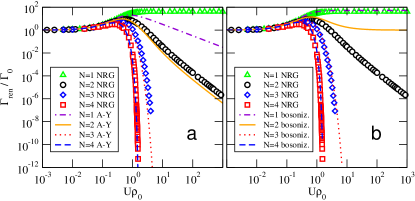
Figure 1: (Color online) Renormalized level width for the IRLM with up to $4$ screening channels, as obtained by the NRG, bosonization, and the AY approach. Here $\Gamma_{0}=\pi\varrho_{0}V^{2}$ with $V/D_{0}=0.02$ (we use $\varrho_{0}D_{0}=1/2$). The AY approach (panel a) works quite well for $N=2,3,4$, but fails for $N=1$. Bosonization (panel b) works well for $N=1,3,4$, but predicts an exact mapping SchillerAndrei07 between $U\to 0$ and $U\to\infty$ for $N=2$, and thus a saturated width. Note that the AY approach systematically underestimates $\Gamma_{\rm ren}$ at large $U$ whereas the opposite is true of bosonization.

We study the IRLM using Wilson’s NRG, bosonization and the AY approach. Since bosonization and the NRG are frequently used, we refer the reader to Refs. bosonization, and Wilson75, for details of these methods. In the following we briefly review the AY approach, which relies on a mapping of the impurity problem onto an effective 1D Coulomb gas of multicomponent charges. The AY mapping is nonperturbative in the Coulomb repulsion $U$, which determines the different charge components through its associated phase shift $\delta=-\arctan(\pi\varrho_{0}U/2)$. Here $\varrho_{0}$ is the bare conduction-electron DoS. The hopping amplitude $V$ fixes the fugacity of the gas, which is given in turn by

$$y=V(\varrho_{0}\tau_{0})^{1/2}\cos\delta.$$ (5)

Here $\tau_{0}=1/D_{0}$ is a short-time cutoff, with $D_{0}$ the bare bandwidth. The $\cos\delta$ that appears in Eq.(5) encodes the DoS renormalization. A similar mapping, only without the $\cos\delta$, can be derived using Abelian bosonization. Incorporating $U$ by means of its associated phase shift, SchillerAndrei07 an identical 1D gas is obtained with $y=V(\varrho_{0}\tau_{0})^{1/2}$.

The Coulomb gas is next treated by progressively increasing the short-time cutoff while simultaneously renormalizing the gas parameters so as to leave the partition function invariant. This results in renormalization-group (RG) equations for the parameters of the Coulomb gas BordaZawadowski07 which are perturbative in the fugacity $y$ (namely, $V$) but nonperturbative in $U$. To illustrate the basic iterative step, suppose that the short-time cutoff has already been increased from its bare value $\tau_{0}=1/D_{0}$ to $\tau>\tau_{0}$. Further increasing the cutoff to $\tau+\delta\tau$ requires two operations: (i) integration over charge pairs whose separation falls in the interval $(\tau,\tau+\delta\tau)$, and (ii) rescaling of $\tau$ by $\tau+\delta\tau$. Consecutive charges, having opposite signs, leave no net charge behind. However, they do possess a dipole moment that acts to screen the interaction between the charges that remain. Integration over the close-by charge pairs can therefore be absorbed into a renormalization of the remaining charges. On the other hand, the rescaling of $\tau$ is absorbed into a renormalization of the fugacity $y$, as described by the following set of RG equations: BordaZawadowski07

$$\frac{dy}{d\ln\tau} = y\left(\frac{1}{2}-z_{0}-\frac{1}{2}\sum_{n=0}^{N-1}z_{n}^{2}\right)\;,$$ (6)

$$\frac{dz_{n}}{d\ln\tau} = 2\left(\delta_{n0}+z_{n}\right)y^{2}\;.$$ (7)

Here $\delta_{n0}$ is the Kronecker delta, while the charge components $z_{n}$ take the bare value $z=2\delta/\pi$. Contrary to usual dynamical scaling equations, the DoS is also modified in this procedure due to the rescaling of $\tau$. However, this difference is only formal. Either strategy can be pursued.

Equation (6) pertains to the fugacity $y$. It can equally be written as a scaling equation for the level width $\Gamma=\pi y^{2}/\tau$, which serves as the low-energy cutoff in the problem. Specifically, the perturbative RG procedure terminates at $1/\tau\sim\Gamma$, when the fugacity $y$ becomes of order $1$. Whether this condition is met or not depends on the values of $N$ and $\delta$. To see this, consider a sufficiently small $y_{0}$ such that the renormalizations of $z_{n}$ can be ignored. Equation (6) then becomes

$$\frac{dy}{d\ln\tau}=\frac{1}{2}\left(1-2z-Nz^{2}\right)y.$$ (8)

Whether $y$ is relevant or not depends on the sign of the expression in the brackets. Since $-1<z<0$ for repulsive interactions, $y$ is always relevant for $N\leq 3$. However, it turns irrelevant for $N>3$ if $U$ is made sufficiently large. The system flows then to a decoupled level. Careful analysis of the transition between a strongly coupled and a decoupled level shows that it is of the Kosterlitz-Thouless type, SBZA08 analogous to the ferromagnetic-antiferromagnetic transition line of the anisotropic Kondo model. Importantly, bosonization and the AY approach predict the same critical coupling $U_{\rm c}$ as $V\to 0$.

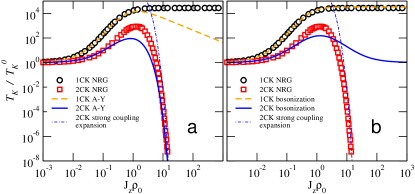
Figure 2: (Color online) The Kondo temperature of the one- and two-channel Kondo model as a function of $J_{z}$ for fixed $\varrho_{0}J_{\perp}=0.1$. While bosonization works quite well for the 1CKM, the AY approach incorrectly predicts a vanishing $T_{K}$ as $J_{z}\to\infty$. The roles are reversed for the 2CKM. Here the AY method is qualitatively correct, whereas bosonization predicts SchillerDeLeo08 an exact mapping between $J_{z}\to 0$ and $J_{z}\to\infty$, and thus a saturated $T_{K}$. The dotted-dashed line shows a one-parameter fit [the prefactor of $\Lambda_{\perp}$ in Eq.(47) of Ref. SchillerDeLeo08, ] to the strong-coupling expansion of the 2CKM.

Solution of Eq.(8) in the regime where $y$ is relevant yields the renormalized level width, or cutoff scale,

$$\Gamma_{\rm ren}\sim D_{0}y_{0}^{2/(1-2z-Nz^{2})}.$$ (9)

Here $y_{0}$ is the bare fugacity of Eq.(5). For either $N=1$ or $N=2$, one can substitute $z\simeq-1$ in Eq.(9) to obtain $\Gamma_{\rm ren}\sim D_{0}y_{0}^{2/(3-N)}$ at large $\varrho_{0}U$. Hence $\Gamma_{\rm ren}$ is strongly suppressed as $\varrho_{0}U\to\infty$ due to the $\cos\delta$ that appears in $y_{0}$. By contrast, $\Gamma_{\rm ren}$ saturates in bosonization, where the DoS renormalization factor is absent.

Figure 1 compares the renormalized level width $\Gamma_{\rm ren}$ of the multichannel IRLM, as obtained by our three methods of interest. Within the NRG, $\Gamma_{\rm ren}$ was defined from the $T\to 0$ charge susceptibility of the level according to $\Gamma_{\rm ren}=1/\pi\chi_{\rm c}$. In the AY approach and bosonization, $\Gamma_{\rm ren}$ was obtained from a full numerical solution of Eqs.(6) and (7), with and without the $\cos\delta$ in Eq.(5).

While both the AY method and bosonization work quite well for $N>2$, only the former approach succeeds in tracing the NRG for $N=2$. Bosonization fails to produce the suppression in $\Gamma_{\rm ren}$ at large $U$, which stems from the renormalized DoS. By contrast, the AY approach fails to generate the saturation in $\Gamma_{\rm ren}$ for $N=1$ and large $U$, which bosonization captures quite well. Hence, the DoS renormalization factor is superfluous in this case. The source of distinction between $N=1$ and $N=2$ is nicely elucidated by a strong-coupling expansion SchillerAndrei07 in $1/U$. Whereas a decoupled entity with local dynamics is formed when $N=1$, for $N=2$ the strong-coupling fixed point is unstable. A renormalized IRLM is recovered, SchillerAndrei07 with dynamics that depends on the renormalized DoS. Relevance of the DoS renormalization depends then on the stability of the strong-coupling fixed point. As shown below, the same criterion applies to the Kondo model.

—Anisotropic single-channel Kondo model. The anisotropic 1CKM has been intensely studied over the years AndersonYuval70 ; FowlerZawadowski71 ; AndersonHamann70 ; Solyom74 as a paradigmatic example for strong correlations. It describes the spin-exchange interaction of an impurity spin $\vec{S}$ with the local conduction-electron spin-density $\vec{s}$, as modeled by the Hamiltonian term

$${\cal H}_{\rm int}=J_{z}S^{z}s^{z}+\frac{J_{\perp}}{2}\left(S^{-}s^{+}+S^{+}s^{-}\right).$$ (10)

In the antiferromagnetic regime, $J_{z}>-|J_{\perp}|$, the system flows to the strong-coupling fixed point of the isotropic model regardless how large the anisotropy is.

Similar to the hopping $V$ in the IRLM, the transverse Kondo coupling $J_{\perp}$ is attached a factor of $\cos^{2}\delta$ with $\delta=-\arctan(\pi\varrho_{0}J_{z}/4)$ upon mapping the 1CKM onto an effective 1D Coulomb gas using the AY approach. This factor, which stems from the form of the electronic Green function, VladarZimanyi88 is absent in bosonization, and is omitted in the original works of Anderson and collaborators. AndersonYuval70 ; AndersonHamann70 Its inclusion has profound implications, as the effect of spin flips (and consequently the Kondo temperature) vanishes in the limit $\delta\to\frac{\pi}{2}$ (i.e., $J_{z}\to\infty$). If these considerations are correct, then the NRG should give the same result as $J_{z}\to\infty$, which turns out not to be the case.

Figure 2 compares the Kondo temperature $T_{K}$ obtained by our three methods of interest. Within the NRG, $T_{K}$ was defined from the $T\to 0$ impurity spin susceptibility according to $T_{K}=1/4\chi_{s}$. In the AY approach and bosonization, it followed from a full numerical solution of the RG equations AndersonHamann70 with and without the $\cos^{2}\delta$ factor attached to $J_{\perp}$. Evidently, bosonization works quite well for the 1CKM, reproducing the saturation of the Kondo temperature as $J_{z}\to\infty$. The AY prediction of a vanishing $T_{K}$ is clearly discredited by the NRG, proving the redundancy of the DoS renormalization factor. As anticipated, a decoupled entity is formed at large $J_{z}$, signaling the stability of the strong-coupling fixed point.

A critical test of our picture is provided by the anisotropic two-channel Kondo model (2CKM), whose strong-coupling fixed point is known to be unstable. Instead, the model flows to an intermediate-coupling, non-Fermi-liquid fixed point, characterized by anomalous thermodynamic and dynamic properties. CoxZawadowski98 Similar to the two-channel IRLM, we expect the DoS renormalization to be essential in this case. The results shown in Fig.2 well support our picture. While bosonization predicts SchillerDeLeo08 an exact mapping between $J_{z}\to 0$ and $J_{z}\to\infty$, and thus a saturated $T_{K}$, the AY approach correctly reproduces the vanishing of $T_{K}$. Though quantitatively less accurate at intermediate $J_{z}$, agreement with the NRG is clearly very good both at small and large coupling.

Above two screening channels, the anisotropic Kondo model undergoes a Kosterlitz-Thouless transition with increasing $J_{z}>0$ to a ferromagnetic-like state. SchillerDeLeo08 Since spin flips are suppressed to zero, the distinction between bosonization and the AY approach looses its significance at strong coupling, similar to the IRLM with $N>3$.

Figure 3: (Color online) Renormalized level width of the one- and two-channel IRLM vs the Kondo temperature of the 1CKM, obtained using the NRG. Here $J_{\perp}=\sqrt{8}V$. As predicted by bosonization, there is close correspondence between the 1CKM and the $N=1$ IRLM upon equating $\sqrt{2}\delta_{z}+\pi(\sqrt{2}-1)/2$ with $\delta_{\rm U}$.

—Comparison of the two models. Prompted by these results, we have set out to carefully test the accepted mapping Schlottmann82 of the one-channel IRLM onto the 1CKM, as the mapping involves large couplings. Within bosonization, one finds the following correspondence of parameters: Mapping $V\leftrightarrow J_{\perp}/\sqrt{8}$ and $\delta_{\rm U}\leftrightarrow\sqrt{2}\delta_{z}+\pi(\sqrt{2}-1)/2$, with $\delta_{\rm U}=-\arctan(\pi\varrho_{0}U/2)$ and $\delta_{z}=-\arctan(\pi\varrho_{0}J_{z}/4)$. Our NRG results for the low-energy scales of both models are summarized in Fig.3. Evidently, there is close correspondence between the two models using the above mapping of parameters, confirming the predictions of bosonization. Note that $T_{K}$ varies by a factor of $30$ in Fig.3. The agreement does not extend to the two-channel IRLM, which similarly flows to a strong-coupling Fermi-liquid fixed point (unlike the non-Fermi-liquid fixed point of the 2CKM). The DoS renormalization factor, absent in the 1CKM, proves essential in this case.

—Conclusions. We have critically examined the accuracy of the AY and bosonization methods away from weak coupling by considering two generic impurity models. Reduction of the conduction-electron DoS, accounted for by the AY approach but absent in bosonization, was shown to be vital in the case of an unstable strong-coupling fixed point, yet superfluous in models where a decoupled entity with local dynamics is formed. The two methods thus display complementary accuracies at strong coupling, controlled by the stability of the strong-coupling fixed point. Accuracy of these powerful methods can thus be significantly enhanced by selectively incorporating the DoS renormalization factor, making them adequate tools for tackling strong-coupling physics.

—Acknowledgments. We are grateful to Natan Andrei for stimulating discussions. This research was supported in part by Hungarian Grants OTKA through project T048782 (L.B. and A.Z.), by the János Bolyai Foundation and the Alexander von Humboldt Foundation (L.B), and by the Israel Science Foundation (A.S.).

References

- (1) See, e.g., P. Nozières and C.T. De Dominicis, Phys. Rev. 178, 1097 (1969).
- (2) J. Kondo, Prog. Theor. Phys. 32, 37 (1964).
- (3) P.W. Vigman and A.M. Finkelstein, Zh. Eksp. Theor. Fiz. 75, 204 (1978) [Sov. Phys. JETP 48, 102 (1978)].
- (4) P. Schlottmann, Phys. Rev. B 25, 4815 (1982).
- (5) C.C. Yu and P.W. Anderson, Phys. Rev B 29, 6165 (1984).
- (6) K. Vladár, A. Zawadowski, and G.T. Zimányi, Phys. Rev. B 37, 2001 (1988), and references therein.
- (7) See, e.g., A.O. Gogolin, A.A. Nersesyan, and A.M. Tsvelik, Bosonization and Strongly Correlated Systems, Cambridge University Press 2004; J. Sólyom, Adv. Phys. 28, 201 (1979).
- (8) P.W. Anderson and G. Yuval, Phys. Rev. B 1, 1522 (1970).
- (9) P.W. Anderson, G. Yuval, and D.R. Hamann, Phys. Rev. B 1, 4464 (1970).
- (10) M. Fowler and A. Zawadowski, Solid State Comm. 9, 471 (1971); A.A. Abrikosov and A.A. Migdal, J. Low Temp. Phys. 3, 471 (1971).
- (11) K.G. Wilson, Rev. Mod. Phys. 47, 773 (1975). For a recent review, see R. Bulla, T. Costi, and T. Pruschke, Rev. Mod. Phys. 80, 395 (2008).
- (12) F. Mezei and A. Zawadowski, Phys. Rev. B 3, 167 (1971).
- (13) T. Giamarchi, C.V. Varma, A.E. Ruckenstein, and P. Nozières, Phys. Rev. Lett 70, 3967 (1993).
- (14) L. Borda, K. Vladár, and A. Zawadowski, Phys. Rev. B 75, 125107 (2007).
- (15) P.W. Anderson, Phys. Rev. Lett. 18, 1049 (1967).
- (16) P. Mehta and N. Andrei, Phys. Rev. Lett. 96, 216802 (2006).
- (17) A. Schiller and N. Andrei, preprint arXiv:0710.0249.
- (18) A. Schiller, L. Borda, A. Zawadowski, and N. Andrei, in preparation.
- (19) J. Sólyom, J. Phys. F: Met. Phys. 4, 2269 (1974).
- (20) D.L. Cox and A. Zawadowski, Adv. Phys. 47, 599 (1998).
- (21) A. Schiller and L. De Leo, Phys. Rev. B 77, 075114 (2008).
- (22) Note that Ref. Schlottmann82, settled with linearizing the phase shifts. It also lacks a factor of in .