The problem of superluminal diffusion of relativistic particles and its phenomenological solution

Abstract

We discuss the problem of superluminal propagation in diffusion of ultra-high energy protons with energy losses taken into account. The phenomenological solution of this problem is found with help of generalized Jüttner propagator, originally proposed for the relativization of Maxwellian gas distribution. It is demonstrated that the generalized Jüttner propagator gives correct expressions in limits of diffusive and rectilinear propagation of the charged particles in magnetic fields, together with the intermediate regime, in all cases without superluminal velocities. This solution, very general for the diffusion, is considered for two particular cases: the diffusion inside stationary objects, like e.g. galaxies, clusters of galaxies etc, and for the expanding universe. The comparison with previously obtained solutions for propagation of UHE protons in magnetic fields is performed.

1 Introduction

Diffusion equation describes many physical processes: thermal conductivity, the Brownian motion, the viscous motion in gases, propagation of charged particles in magnetic field and others. Our main interest is the diffusion of charged relativistic particles (cosmic rays). For collisional processes in gas, the diffusion equation can be obtained from kinetic equations (Landau & Lifshitz, v.10, 2001). The derivation of diffusion equation for motion of charged particles in magnetic fields is given in (Berezinsky et al., 1990).

In the extreme case, neglecting energy losses of particles and convection, assuming the diffusion coefficient $D(t,\vec{r})$ independent of the time and space coordinates, the diffusion equation for the space density of particles $n(\vec{r},t)$ has a simple form:

$$\frac{\partial}{\partial t}n(\vec{r},t)-D\nabla^{2}n(\vec{r},t)=Q(\vec{r},t),$$ (1)

where $Q(\vec{r},t)$ is the generation function. The diffusion coefficient is defined phenomenologically through the flux density of particles as

$$\vec{j}(\vec{r},t)=-D\nabla n(\vec{r},t).$$ (2)

Both diffusion equation (1) and definition of the flux density do not know about light speed $c$ and in fact result in superluminal motion. A common example demonstrating it (see e.g. (Dunkel et al., 2007)) can be described as follows. From Eq. (2) one can find the streaming velocity $\vec{u}(\vec{r},t)$, determined from $\vec{j}=n\vec{u}$, as

$$\vec{u}=-D\nabla n/n.$$ (3)

For the stationary ($\partial n/\partial t=0$) spherically symmetric diffusion one has from Eq. (1)

$$n=\frac{Q}{4\pi rD}\;\;\;\mbox{and}\;\;\;\frac{\partial n}{\partial r}=-\frac{Q}{4\pi r^{2}D},$$ (4)

and finally, using the definition of the diffusion length $l_{d}$ from $D\sim cl_{d}$ for diffusion of relativistic particles with velocities $v\sim c$, one obtains from (3) and (4)

$$u\sim c\;\frac{l_{d}}{r},$$ (5)

which at $r<l_{d}$ results in $u>c$.

Another way to demonstrate the problem of superluminal propagation in diffusion is given by consideration of the average displacement of a particle in the diffusive regime, $r^{2}\sim Dt$. One obtains for average velocity of displacement $v\sim r/t\sim c(l_{d}/r)$ with the same problem as above. From now on we shall refer to this problem as superluminal diffusion.

From the practical point of view the described problem of superluminal diffusion, widely discussed in the literature, can be in many cases easily avoided. In particular, for diffusion of charged particles in magnetic fields, a particle deflects at length $l_{d}$ on average by angle $\theta\sim 1$ and the movement of a particle at $r\lesssim l_{d}$ can be considered as quasi-rectilinear as long as the energy spectra are concerned and as we did in our works (Berezinsky & Gazizov, 2006, 2007). In these works, discussing the diffusion of ultra-high energy cosmic ray (UHECR) protons, we have met a more serious problem of superluminal propagation connected with inclusion of proton energy losses.

The diffusion equation for protons with a source at $\vec{r}=\vec{r}_{g}$, energy losses in the form $dE/dt=-b(E)$ and with time-independent diffusion coefficient $D(E)$, reads

$$\frac{\partial}{\partial t}n_{p}(E,\vec{r},t)-D(E)\nabla^{2}n_{p}(E,\vec{r},t)-\frac{\partial}{\partial E}\left[b(E)n_{p}(E,\vec{r},t)\right]=Q(E,t)\delta^{3}(\vec{r}-\vec{r}_{g}).$$ (6)

The solution of this equation was found by Syrovatsky (Syrovatsky, 1959) as

$$n_{p}(E,\vec{r},\vec{r}_{g})=\frac{1}{b(E)}\int\limits_{E}^{\infty}dE_{g}Q(E_{g})\frac{\exp\left[-(\vec{r}-\vec{r}_{g})^{2}/4\lambda(E,E_{g})\right]}{\left[4\pi\lambda(E,E_{g})\right]^{3/2}},$$ (7)

where $n_{p}$ is the space density of relativistic protons, $E$ is the observed energy, $E_{g}$ is the generation energy of a proton in the source, and $\lambda(E,E_{g})$ given by

$$\lambda(E,E_{g})=\int\limits_{E}^{E_{g}}dE^{\prime}\;\frac{D(E^{\prime})}{b(E^{\prime})},$$ (8)

has a meaning of a distance squared traversed by a proton in a given direction during the time, when the proton energy decreases from $E_{g}$ to $E$.

The superluminal diffusion in solution (7) is immediately seen from the fact that it is the solution of Eq. (6) only when the lower limit of integration is the observed energy $E_{g}^{{\rm min}}=E$. One may prove it substituting (7) into (6). In particular, at any other lower limit $E_{g}^{\rm min}$ the delta-function in the r.h.s. of Eq. (6) is not reproduced.

Thus, the minimum generation energy at distance $r$ in the solution of Eq. (6) equals to the observed energy $E$ and it can be interpreted in the unique way: the propagation time $\tau\rightarrow 0$ and thus the energy loss of a particle is absent. It implies the velocity of a particle $v\rightarrow\infty$.

The physical value of the minimal generation energy $E_{g}^{{\rm min}}(E,r)$ is given by the rectilinear propagation and it can be easily calculated if $b(E)=-dE/dt$ is known. But with this $E_{g}^{{\rm min}}$ Eq. (7) is not any more the solution of Eq. (6). In the left panel of Fig. 1 the unphysical region of the solution (7) with superluminal velocity is shown as the hatched area.

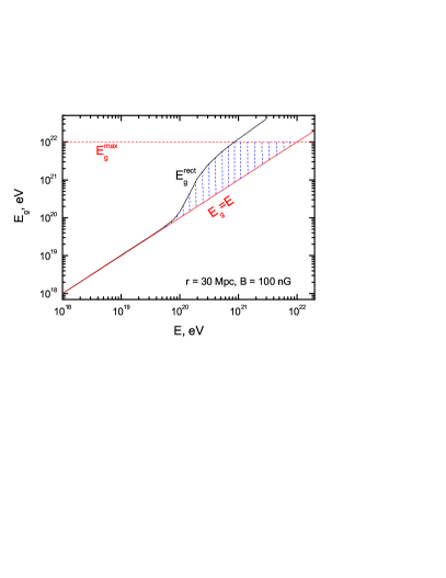
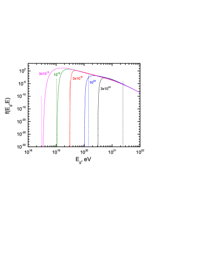
Figure 1: The superluminal propagation problem in the Syrovatsky solution caused by energy losses of UHE protons for $B_{c}=100$ nG and distance to the source $r=30$ Mpc. In the left panel is shown the region in ($E_{g}\;,E$) plane (above $E_{g}=E$ line) allowed by Eq. (7). The line $E_{g}=E_{g}^{{\rm rect}}(E,r)$ corresponds to rectilinear propagation and to the physical lower limit in the solution (7). The hatched region between $E_{g}=E$ and $E_{g}=E_{g}^{\rm rect}$ corresponds to superluminal velocities. For $E\lesssim 1\times 10^{20}$ eV the solutions practically do not have superluminal velocities. In the right panel the integrand of Eq. (7) is shown as function of $E_{g}$ for fixed $E$ with values indicated by the numbers, given in eV. The dashed lines show the rectilinear physical lower limits $E_{g}^{\rm min}$. At $E\lesssim 1\times 10^{20}$ eV the regions below these limits, i.e. with $v>c$ are negligibly small, while at $E>1\times 10^{20}$ eV they give considerable contribution to Eq. (7).

2 The problem of superluminal diffusive propagation of UHECR and how it has been eliminated

From the formal mathematical point of view the superluminal propagation exists always in the solutions of the non-relativistic diffusion equations, but very often the contribution of unphysical regions to the solution is negligibly small (e.g. in heat conductivity). In these cases one may say that diffusion equation gives the correct description of the considered physical phenomenon. It is similar to validity of the Maxwell distribution for molecules in low-temperature gas (this analogy will be considered in the next section), where formally there are particles with velocities $v\to\infty$.

In our works (Aloisio & Berezinsky, 2004, 2005) on diffusion of UHE protons in static universe and in the works (Berezinsky & Gazizov, 2006, 2007) on diffusion in the expanding universe we recognized the problem of superluminal propagation and eliminated it using the following recipes:

(i) For calculation of flux from a source at distance $r\lesssim l_{d}(E)$ for protons with energies $E$ we used the rectilinear propagation. Then the problem of superluminal diffusion disappears, but a technical problem of sewing the rectilinear and diffusive solutions arises, since the rectilinear propagation starts at $r\sim l_{d}(E)$, while diffusive regime begins at $r\sim 6l_{d}(E)$. In the paper (Aloisio & Berezinsky, 2005) we used some smooth interpolation between two regimes, while in the paper (Berezinsky & Gazizov, 2007) we used for transition the fixed energy $E_{t}(r)$, where rectilinear and diffusive fluxes are equal. It was done intentionally, because the energy of transition appeared in the calculated diffuse spectrum as a feature, which indicates the change of the propagation regime.

(ii) The superluminal propagation is caused also by energy losses of particles during diffusion, and it appears as $E_{g}^{\rm min}=E$ in Eq. (7). This problem is ameliorated by presence of the magnetic horizon (see below): the problem of superluminal diffusion is most severe for the sources at largest distances beyond the magnetic horizon, while contribution of these sources to the observed diffuse flux is small.

According to our calculations the picture for propagation of UHE protons in extragalactic magnetic fields looks as follows. At low energies diffusion dominates. At high energies, determined by energy dependence of the diffusion length $l_{d}(E)$ and by size of horizon $r_{\rm hor}(E)$, the propagation changes to (quasi)rectilinear, which has no problem with superluminal propagation. This picture is valid for magnetic fields with the critical values $B_{c}$ (see below) between $0.01-10$ nG. For the fields $B_{c}\gtrsim 100$ nG the superluminal signal appears at the highest energies in the diffuse spectrum (see Fig. 1). The fields $B_{c}\lesssim 1.6\times 10^{-3}$ nG provide quasi-rectilinear propagation for all protons at energies $E\geq 1\times 10^{17}$ eV, while at lower energies the diffusion becomes unavoidable (Berezinsky & Gazizov, 2007). For a reasonably low field $B_{c}\approx 0.01$ nG, diffusion becomes valid at $E\lesssim 1\times 10^{18}$ eV.

Some technical details and numerical results on the problem of superluminal diffusion are in order.

We have considered diffusion of UHECR in magnetized turbulent plasma with random magnetic field, and with the coherent magnetic field $B_{c}$ on the basic linear scale $l_{c}$. It determines the critical energy $E_{c}\approx 1\times 10^{18}(B_{c}/1~{}{\rm nG})(l_{c}/1~{}{\rm Mpc})$ eV, calculated from relation $r_{L}(E_{c})\approx l_{c}$, where $r_{L}(E)$ is the Larmor radius of particle in magnetic field $B_{c}$. The diffusion length $l_{d}(E)=l_{c}(E/E_{c})^{2}$ at $E>E_{c}$ for all spectra of turbulence and $l_{d}(E)=l_{c}(E/E_{c})^{n}$ at $E<E_{c}$ with $n=1/3$ and $n=1$ for the Kolmogorov and Bohm diffusion, respectively. At intermediate energies the interpolation of $l_{d}(E)$ between these two regimes was used. For low magnetic field $B_{c}\leq 1$ nG and at $E>E_{c}$ the diffusion length $l_{d}(E)$ becomes very large at high energy and propagation of UHE protons becomes rectilinear at all highest energies. The superluminal propagation thus disappears at all energies above the energy of transition $E_{tr}$ from diffusive to rectilinear regime. In calculation of $E_{{\rm tr}}$ the magnetic horizon is involved (Aloisio & Berezinsky, 2005; Aloisio et al., 2007) (for physical discussion of magnetic horizon see (Parizot, 2004)). Magnetic horizon is determined as a distance traversed by a particle during the age of a universe $t_{0}$:

$$r^{2}_{{\rm hor}}=\int\limits_{0}^{t_{0}}dt\;D[E_{g}(E,t)],$$ (9)

where $E_{g}(E,t)$ is the energy that a particle has at time $t$, if its energy at $t=t_{0}$ is $E$. Putting $dt=-dE_{g}/b(E_{g})$ in Eq. (9) we obtain

$$r^{2}_{{\rm hor}}=\int\limits_{E}^{E_{{\rm max}}}dE_{g}\frac{D(E_{g})}{b(E_{g})},$$ (10)

where $E_{\max}=\min[E_{g}(E,t_{0}),E_{\max}^{{\rm acc}}]$, and $E_{\max}^{{\rm acc}}$ is the maximum acceleration energy.

In $r^{2}_{{\rm hor}}$ one may recognize the Syrovatsky variable $\lambda(E,E_{g})$ at $E_{g}=E_{\max}$. The Syrovatsky solution (7) knows about the horizon suppression of $n(E,r)$ at distance $r\geq\sqrt{\lambda(E,E_{g})}$ by exponential factor $\exp(-r^{2}/4\lambda)$.

The energy of transition from diffusive to rectilinear propagation is determined for diffuse fluxes by condition $l_{d}(E)\gtrsim r_{{\rm hor}}(E)$, or $l_{d}^{2}(E_{{\rm tr}})\sim\lambda(E_{{\rm tr}},E_{\max})$ with $E_{\max}$ defined as above.

If magnetic field is very strong, $B_{c}\sim 100$ nG (Aloisio & Berezinsky, 2004), and hence $E_{c}\sim 10^{20}$ eV, the diffusive regime continues up to very high energies and contribution of unphysical solutions (with $v>c$) appears. In Fig. 1 the integrand of Eq. (7) is shown as a function of $E_{g}$ for $B_{c}=100$ nG and distance to a source $r=30$ Mpc. The unphysical regions with $v>c$ are negligibly small at $E\leq 3\times 10^{19}$ eV, but is large at $E=3\times 10^{20}$ eV. In this case we limited our consideration by energies $E<1.2\times 10^{20}$ eV (see Fig. 6 in (Aloisio & Berezinsky, 2004)).

3 Approach to solution of the superluminal propagation problem

The most radical way to eliminate the superluminal signal in non-relativistic diffusion equation is given by relativization of the diffusion equation similar to relativization of the Schrödinger equation in quantum mechanics. However, after more than 70 years of efforts in this direction no successful solution has been found (see (Dunkel et al., 2007) for review and references). In this paper we shall follow another approach first suggested by F. Jüttner (Jüttner, 1911) for the relativization of the Maxwellian distribution of particles. We apply this method to the Green function of the diffusion equation.

In the work (Dunkel et al., 2007) it was observed that the problem of relativization of the Maxwell distribution is identical to the relativization of diffusion propagator (the Green function). The normalized (per unit phase volume) probability density function of the Maxwell distribution of particles with mass $m$ and temperature $T$ is given by

$$P_{M}(v)=\left(\frac{m}{2\pi kT}\right)^{3/2}\exp\left(-\frac{mv^{2}}{2kT}\right).$$ (11)

Changing $v\to x$ and $kT/m\to 2Dt$ one obtains the Green function of the diffusion equation (1):

$$P_{\rm diff}(r,t)=\frac{1}{(4\pi Dt)^{3/2}}\;\exp\left(-\frac{r^{2}}{4Dt}\right),$$ (12)

where $r$ is a distance to the source and $D$ is time-independent diffusion coefficient.

Therefore, one can use for the diffusive Green function the Jüttner distribution, where superluminal velocities are absent.

We start with the phenomenological definition of the propagation function (propagator). Let us consider first the static universe or more generically an extended stationary object like a galaxy or a cluster of galaxies. The propagation of the charged particles in magnetic fields may be described with help of propagator $P(E,t,r)$, where $E$ is the observed energy, $t$ is the propagation time and $r$ is the distance to a source. The definition of the propagator is given by

$$n(E,r)=\int_{0}^{\infty}dt\;Q[E_{g}(E,t),t]\;P(E,t,r)\;\frac{dE_{g}}{dE}(E,t),$$ (13)

where $n(E,r)$ is the observed space density of particles, $E_{g}(E,t)$ is energy of a particle at time $t$, analytic expression for $dE_{g}/dE$ is given in (Berezinsky, Gazizov & Grigorieva, 2006), and $Q(E,t)$ is the source generation function.

The propagator $P(E,t,r)$ can be thought of as a Green function of an unknown relativistic equation.

For rectilinear propagation of ultrarelativistic particles with $v\approx c$ the propagator is given by

$$P(E,t,r)=\frac{1}{4\pi c^{3}t^{2}}\;\delta(t-\frac{r}{c})\;,$$ (14)

and Eq. (13) results in

$$n(E,r)=\frac{Q[E_{g}(E,r/c),r/c]}{4\pi cr^{2}}\;\frac{dE_{g}}{dE},$$ (15)

which coincides with the expression obtained from conservation of number of particles.

For diffusive propagation the propagator can be obtained from the Syrovatsky solution (7) as

$$P(r,t)=\frac{1}{[4\pi\lambda(E,t)]^{3/2}}\exp\left[-\frac{r^{2}}{4\lambda(E,t)}\right],$$ (16)

where

$$\lambda(E,t)=\int_{0}^{t}dt^{\prime}D[E(t^{\prime})]=\int_{E}^{E_{g}(t)}dE^{\prime}\;\frac{D(E^{\prime})}{b(E^{\prime})}$$ (17)

and $D(E)$ is the diffusion coefficient; $b(E)=-dE/dt$ is the energy loss of a particle. The density of particles $n_{\rm diff}(E,r)$ is given by Eq. (13).

Both propagation functions $P_{\rm rec}(E,t,r)$ and $P_{\rm diff}(E,t,r)$ are normalized by unity

$$\int dVP(E,t,r)=1$$ (18)

and thus they have a meaning of probability to find a particle in a unit volume at distance $r$ from a source at time $t$ after emission. It is easy to see from Eqs. (14) and (15) that $P(E,t,r)$ has the correct dimension $[P]=L^{-3}$.

The Jüttner distribution in terms of $r=v$ and $2Dt=kT/m$, as was described above, has been given in (Dunkel et al., 2006) as

$$P_{J}(E,t,r)=\frac{\theta(ct-r)}{(ct)^{3}Z\left(\frac{c^{2}t}{2D}\right)\left[1-\left(\frac{r}{ct}\right)^{2}\right]^{2}}\;\exp\left[-\frac{\frac{c^{2}t}{2D}}{\sqrt{1-\left(\frac{r}{ct}\right)^{2}}}\right],$$ (19)

where

$$Z(y)=4\pi K_{1}(y)/y$$ (20)

with $K_{1}(y)$ being the modified Bessel function. One may observe that the superluminal propagation with $v=r/t>c$ is forbidden for this propagator.

Instead of the Jüttner function (19) we introduce the generalized Jüttner function $P_{gJ}(E,t,r)$, imposing to it two limiting conditions of transition to rectilinear propagator (14) and the Syrovatsky propagator (12), and keeping the condition of subluminal velocities $r\leq ct$. For this purpose we transform the Eq. (19) as follows:

$$\frac{c^{2}t}{2D}\rightarrow\frac{c^{2}t^{2}}{2\lambda[E_{g}(E,t)]}\equiv\alpha(t),$$ (21)

and use instead of $t$ the new variable

$$\xi(t)=r/ct,$$ (22)

where $\lambda[E_{g}(E,t)]$ is given by Eq. (17). Note that the both new quantities are dimensionless.

The generalization imposed by Eq. (21) is motivated by the time-dependent diffusion coefficient $D[E_{g}(t)]$ and by the presence of energy losses. In this case we generalize the implicit quantity $D\times t$ in the Jüttner distribution (19) to $\int D(t)dt=\lambda(E,t)$ given by Eq. (17). As a result we have

$$\frac{c^{2}t}{2D}=\frac{c^{2}t^{2}}{2Dt}\rightarrow\frac{c^{2}t^{2}}{2\int D(E,t)dt}=\frac{c^{2}t^{2}}{2\lambda(E,t)}\equiv\alpha(E,t).$$ (23)

In terms of $\xi$ and $\alpha(E,t)$ the generalized Jüttner function $P_{gJ}(E,t,x)$ and density of particles $n(E,r)$ are given by:

$$P_{gJ}(E,t,r)=\frac{\theta(1-\xi)}{4\pi(ct)^{3}}\;\frac{1}{(1-\xi^{2})^{2}}\;\frac{\alpha(E,\xi)}{K_{1}[\alpha(E,\xi)]}\;\exp\left[-\frac{\alpha(E,\xi)}{\sqrt{1-\xi^{2}}}\right],$$ (24)

$$n(E,r)=\frac{1}{4\pi cr^{2}}\int\limits_{\xi_{{\rm min}}}^{1}d\xi\;\frac{Q[E_{g}(E,\xi)]}{(1-\xi^{2})^{2}}\;\xi\;\frac{\alpha(E,\xi)}{K_{1}[\alpha(E,\xi)]}\;\exp\left[-\frac{\alpha(E,\xi)}{\sqrt{1-\xi^{2}}}\right]\frac{dE_{g}}{dE}.$$ (25)

Now we prove that Eqs. (24) and (25) have the correct rectilinear and diffusive asymptotic behavior.

Consider first the high energy regime, where rectilinear propagation is expected. At $E^{\prime}>E_{c}$ the diffusion coefficient increases with $E^{\prime}$ as $D(E^{\prime})\propto(E^{\prime}/E_{c})^{2}$, while $E^{\prime}(t)$ increases exponentially with time (Aloisio & Berezinsky, 2004). As a result $\lambda(E,t)$ increases exponentially with time too, providing small $\alpha$ from Eq. (23) and (quasi)rectilinear propagation. On the other hand from Eq. (22) we have $\xi(t)\approx 1$ as the second condition of thus (quasi)rectilinear propagation. We impose both of these conditions to Eq. (25). Using $\xi_{{\rm min}}=1-\varepsilon$ with $\varepsilon\ll 1$ and

$$\alpha/K_{1}(\alpha)\approx\alpha^{2},$$ (26)

valid for $\alpha\ll 1$, one obtains

$$n(E,r)=\frac{A}{4\pi cr^{2}}\;Q\left[E_{g}\left(\frac{r}{c}\right)\right]\frac{dE_{g}}{dE}$$ (27)

with

$$A=\int\limits_{1-\varepsilon}^{1}\xi d\xi\frac{\alpha^{2}}{(1-\xi^{2})^{2}}\;\exp\left(-\frac{\alpha}{\sqrt{1-\xi^{2}}}\right)=\int\limits_{y_{{\rm min}}}^{\infty}ye^{-y}dy=1,$$ (28)

where $y=\alpha/\sqrt{1-\xi^{2}}$, $y_{{\rm min}}\rightarrow 0$ with $\alpha\rightarrow 0$. Thus, the regime (27) is indeed rectilinear.

Now consider the low-energy regime in Eq. (24). At small $E$ and $r\gg l_{\rm diff}(E)$ the diffusive regime, free of the superluminal-signal problem, is valid, and we demonstrate that the generalized Jüttner propagator reproduces the Syrovatsky propagator, given by Eq. (7). Let us first determine the range of parameters $\xi$ and $\alpha$ which corresponds to the diffusion, described by the Syrovatsky solution. The low $E$ corresponds to small $\lambda(E,t)$, and large enough $t$ provides $r\gg l_{\rm diff}(E)$. Therefore we have $\alpha=ct/\sqrt{\lambda}\gg 1$. On the other hand $\sqrt{\lambda(E,t)}>r$ provides the considerable contribution to the observed flux from a source at distance $r$ and thus we have

$$\xi=\frac{r}{ct}<\frac{\sqrt{\lambda}}{ct}=\frac{1}{\sqrt{\alpha}}\ll 1.$$ (29)

With these restrictions on $\alpha$ and $\xi$ we compute now $P_{gJ}(E,t,r)$ using Eq. (24). At $\alpha\gg 1$ one has

$$\alpha/K_{1}(\alpha)\approx\sqrt{\frac{2}{\pi}}\alpha^{3/2}e^{\alpha}.$$ (30)

Using $\exp(-\alpha/\sqrt{1-\xi^{2}})\approx\exp[-\alpha(1+\xi^{2}/2)]$ we obtain from (24) after simple calculations

$$P(E,t,r)=\frac{\theta(ct-r)}{\left[4\pi\lambda(E,t)\right]^{3/2}}\;\exp\left[-\frac{r^{2}}{4\lambda(E,t)}\right],$$ (31)

which coincides with the Syrovatsky propagator (16).

However, it should be demonstrated that the space density of particles is also reproduced correctly. Putting $P(E,t,r)$ from (31) into (13) we obtain indeed the Syrovatsky solution (7), but with $E_{g}^{\rm min}(r)$ as lower limit of integration instead of $E$ in the Syrovatsky solution, where $E_{g}^{\rm min}(r)$ corresponds to the rectilinear propagation $ct=r$. At very low energy $E_{g}^{\rm min}(r)\to E$ (see e.g. Fig. 1) and both solutions coincide.

As a matter of fact Jüttner found two versions of relativization of the Maxwell distribution. His second propagator results in the generalized propagator given by

$$P_{gJ}(E,t,r)=\frac{\theta(1-\xi)}{4\pi(ct)^{3}}\;\frac{1}{(1-\xi^{2})^{5/2}}\;\frac{\alpha(E,\xi)}{K_{2}[\alpha(E,\xi)]}\;\exp\left[-\frac{\alpha(E,\xi)}{\sqrt{1-\xi^{2}}}\right].$$ (32)

The difference between calculated UHE proton fluxes for both cases is less than 0.2%. In the following we discuss the case of propagator (24).

Therefore, the proposed generalized Jüttner propagator (24) has the correct asymptotic behavior (rectilinear at high energies and diffusive at low energies). It interpolates between these two regimes without superluminal velocities. The recent numerical simulations have confirmed the Jüttner distribution of relativistic particles (Cubero et al., 2007), which is generalized in our paper for the time distribution of the charged particles propagating in magnetic fields.

4 Propagation of ultra-relativistic particles in magnetic fields in expanding universe

Charged ultra-relativistic particles propagating in the expanding universe scatter in magnetic fields. Like in the previous section, where stationary flat space was considered (e.g. a galaxy, or static universe), in the expanding universe there are two extreme modes for propagation in magnetic field: the (quasi)rectilinear in the highest energy limit and the diffusive in the low-energy limit. For these limits we follow the works (Berezinsky & Gazizov, 2006, 2007), where cosmological effects have been properly included.

For diffusive propagation of particles from a single source located at the comoving coordinate $\vec{x}_{g}$ with a generation function $Q(E,t)$ the diffusion equation has been derived in the form:

$$\frac{\partial n}{\partial t}-b(E,t)\;\frac{\partial n}{\partial E}+3H(t)\;n-\frac{\partial b(E,t)}{\partial E}\;n-\frac{D(E,t)}{a^{2}(t)}\;\nabla^{2}_{x}n=\frac{Q(E,t)}{a^{3}(t)}\;\delta^{3}(\vec{x}-\vec{x}_{g}),$$ (33)

where the cosmological basis $(\vec{x},t)$ is used, $n(E,t,\vec{x})$ is the space density of the particles, $b(E,t)=-dE/dt$ gives the sum of collisional energy losses, $b_{{\rm int}}(E)$, and adiabatic energy losses $H(t)E$, $H(t)$ is the Hubble parameter, $D(E,t)$ is a diffusion coefficient and $a(t)$ is the scaling factor of the expanding universe.

It was shown that the solution to Eq. (33) reduces to a quadrature. Introducing the analog of the Syrovatsky variable

$$\lambda(E,t,t^{\prime})=\int\limits_{t^{\prime}}^{t}dt^{\prime\prime}\;\frac{D(\mathcal{E}^{\prime\prime},t^{\prime\prime})}{a^{2}(t^{\prime\prime})},$$ (34)

where $\mathcal{E}=E_{g}(E,t,t^{\prime})$ is a solution of the characteristic equation, the solution to Eq. (33) is given by

$$n(t_{0},\vec{x},E)=\int_{0}^{z_{g}}dz\left|\frac{dt}{dz}\right|Q[E_{g}(E,z),z]\times\frac{\exp\left[-(\vec{x}-\vec{x}_{g})^{2}/4\lambda(E,z)\right]}{\left[4\pi\lambda(E,z)\right]^{3/2}},$$ (35)

where $z$ is a redshift, $t_{0}$ is an age of the universe corresponding to $z=0$, $z_{g}$ is the maximum redshift at which a source is present, $dt/dz=-1/[(1+z)H(z)]$, and $E_{g}(E,z)$ is the generation energy in the source.

The equation describing the rectilinear propagation reads (Berezinsky & Gazizov, 2006):

$$\frac{\partial n}{\partial t}-b(E,t)\frac{\partial n}{\partial E}+3H(t)\;n-\frac{\partial b(E,t)}{\partial E}\;n+\frac{c\vec{e}}{a(t)}\;\frac{\partial n}{\partial\vec{x}}=\frac{Q(E,t)}{a^{3}(t)}\;\delta^{3}(\vec{x}-\vec{x}_{g}),$$ (36)

where $\vec{e}$ is a unit vector in the direction of propagation. The solution of Eq. (36) is given by

$$n(t_{0},E)=\frac{Q(E_{g},t_{g})}{4\pi c\;x_{s}^{2}\;(1+z_{g})}\frac{dE_{g}}{dE},$$ (37)

where $x_{s}$ is the comoving distance to a source.

To use the generalized Jüttner distribution for the expanding universe we must modify the parameters $\alpha(t)$ and $\xi(t)$ introduced in Section 3.

To provide cosmologically invariant character of the parameters it is natural to substitute $ct$ by the comoving length of the particle trajectory $\zeta(t)$:

$$\zeta(t)=\int_{t}^{t_{0}}\frac{cdt}{a(t)}=\frac{c}{H_{0}}\int_{0}^{z_{g}}\frac{dz}{\sqrt{\Omega_{m}(1+z)^{3}+\Omega_{\Lambda}}}.$$ (38)

Now we obtain $\alpha(t)$ from the original quantity $c^{2}\tau/2D$ in the Jüttner distribution (Dunkel et al., 2006), where $\tau$ is propagation time, as

$$\frac{c^{2}\tau}{2D}=\frac{c^{2}\tau^{2}}{2D\tau}\rightarrow\frac{\zeta^{2}(t)}{2\lambda(E,t)}\equiv\alpha(E,t),$$ (39)

and use a new variable $\xi$ instead of $t$:

$$\xi(t)=x_{s}/\zeta(t).$$ (40)

For rectilinear propagation $\xi(t)=1$ holds as before.

In terms of the variables $\alpha$ and $\xi$ defined by Eqs. (39), (40) the propagator $P_{J}(E,t,x_{s})$ and particle space density $n(E,x_{s})$ have the form similar to Eqs. (24) and (25):

$$P_{gJ}(E,t,x_{s})=\theta(1-\xi)\;\frac{\xi^{3}}{x_{s}^{3}(1-\xi^{2})^{2}}\;\frac{\alpha}{4\pi K_{1}(\alpha)}\exp\left(-\frac{\alpha}{\sqrt{1-\xi^{2}}}\right).$$ (41)

$$n(E,x_{s})=\frac{1}{4\pi cx_{s}^{2}}\int\limits_{\xi_{{\rm min}}}^{1}\frac{\xi d\xi}{1+z(\xi)}\;\frac{Q[E_{g}(E,\xi)]}{(1-\xi^{2})^{2}}\;\frac{\alpha}{K_{1}(\alpha)}\exp\left(-\frac{\alpha}{\sqrt{1-\xi^{2}}}\right)\frac{dE_{g}}{dE}.$$ (42)

The rectilinear case corresponds to $\xi\approx 1$ and $\alpha\ll 1$. Integral (42) can be evaluated using $\alpha/K_{1}(\alpha)\approx\alpha^{2}$ at $\alpha\ll 1$ and integrating over $\xi$ in a narrow range over $\xi\approx 1$. One obtains Eq. (37) as it is expected.

The diffusive regime corresponds to $\alpha\gg 1$ and $\xi<1$. Using $\alpha/K_{1}(\alpha)$ as given by Eq. (30) one obtains for the propagator the correct diffusion expression

$$P_{gJ}(E,x)=\frac{\exp\left[-x^{2}/4\lambda(E,t)\right]}{[4\pi\lambda(E,t)]^{3/2}}.$$ (43)

Thus, the generalized Jüttner propagator (24) has the correct asymptotic form in rectilinear and diffusive regimes again, providing the interpolation between them without superluminal velocities.

5 UHECR diffuse spectra in the generalized Jüttner approximation

In this section we calculate the diffuse spectra of UHE protons propagating in magnetic fields in the expanding universe and compare them with the calculations of (Berezinsky & Gazizov, 2007), where such spectra have been calculated for diffusive propagation with transition to rectilinear propagation at highest energies. The proposed generalized Jüttner approximation allows both for diffusive and rectilinear propagation at low and high energies, respectively, and provides the interpolation between them based on mathematical analogy between Maxwellian and diffusion distribution (see (Dunkel et al., 2006) and Eqs. (11), (12)).

We start our discussion with the universal diffuse spectrum valid for homogeneous distribution of the sources and for all modes of propagation. This spectrum can be calculated from the conservation of number of particles as

$$n(E)dE=\int_{t_{\rm min}}^{t_{0}}dt\;n_{s}\;Q[E_{g}(E,t)]\;dE_{g},$$ (44)

where $n_{s}$ is the source density per unit comoving volume. According to the propagation theorem (Aloisio & Berezinsky, 2004) this spectrum is independent of mode of particle propagation, and spectrum calculated for any specific mode of propagation must converge to the universal one, when distances between sources become less than any characteristic length involved, e.g. the diffusion length. Therefore, the spectrum (42) integrated over space coordinates $x_{s}$ as

$$n(E)=\int_{0}^{\infty}4\pi x_{s}^{2}dx_{s}n_{s}n(E,x_{s})$$ (45)

must coincide with the universal spectrum (44). This fact can be easily demonstrated using

$$\int_{0}^{\infty}4\pi x_{s}^{2}\;dx_{s}\;P_{gJ}(E,t_{0},x_{s})=1\;,$$ (46)

and relations

$$\xi=\frac{x_{s}}{\zeta}\;\;\;{\rm and}\;\;\;d\xi=-\frac{x_{s}}{\zeta^{2}}\;\frac{c\;dt}{a(t)}.$$ (47)

The calculated universal spectrum is plotted in Fig. 2.

We calculate now the diffuse flux using the particle density from a single source given by Eq. (42) and assuming the lattice distribution of the sources in the coordinate space $x$ with lattice parameter (the source separation) $d$ and a power-law generation spectrum for a single source,

$$Q_{s}(E)=\frac{q_{0}(\gamma_{g}-2)}{E_{0}^{2}}\left(\frac{E}{E_{0}}\right)^{-\gamma_{g}},$$ (48)

where $E_{0}$ is the normalizing energy, for which we will use $1\times 10^{18}$ eV and $q_{0}$ has a physical meaning of a source luminosity in protons with energies $E\geq E_{0}$, $L_{p}(\geq E_{0})$. The corresponding emissivity $\mathcal{L}_{0}=q_{0}/d^{3}$, i.e. the energy production rate in particles with $E\geq E_{0}$ per unit comoving volume, may be used to fit the observed spectrum by the calculated one.

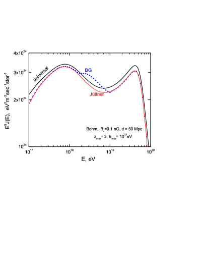
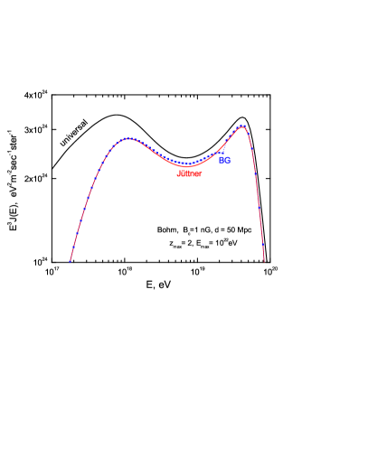
Figure 2: Comparison of the Jüttner solution with the combined diffusive and rectilinear solution (BG dotted curves) from work (Berezinsky & Gazizov, 2007). The left panel shows the case $B_{c}=0.1$ nG, and the right panel $B_{c}=1$ nG, the distance between sources $d=50$ Mpc in both cases and $\gamma_{g}=2.7$. The universal spectrum is also presented for $\gamma_{g}=2.7$. The features seen in the BG spectra are artifacts produced by assumption about transition from diffusive to rectilinear propagation (see text). These features are small: note the large scale on the ordinate axis.

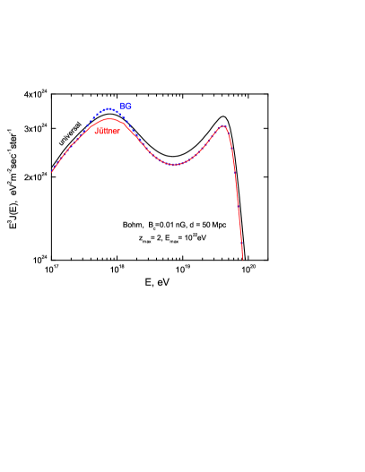
Figure 3: The same as in Fig. 2 for $B_{c}=0.01$ nG.

Using Eq. (42) we obtain the diffuse spectrum as

$$J_{p}(E)=\frac{c}{4\pi H_{0}}\ \frac{q_{0}(\gamma_{g}-2)}{E_{0}^{2}}\sum_{s}\frac{1}{4\pi cx_{s}^{2}}\int\limits_{\xi_{{\rm min}}}^{1}\frac{\xi_{s}d\xi_{s}}{1+z(\xi_{s})}\;\frac{[E_{g}(E,\xi_{s})]^{-\gamma_{g}}}{(1-\xi_{s}^{2})^{2}}\;\frac{\alpha}{K_{1}(\alpha)}\;\exp\left(-\frac{\alpha}{\sqrt{1-\xi_{s}^{2}}}\right)\frac{dE_{g}}{dE}.$$ (49)

For the aim of comparison we use in calculations the same magnetic field and its evolution with redshift $z$ as in the paper (Berezinsky & Gazizov, 2007), namely we parametrize the evolution of magnetic configuration $(l_{c},B_{c})$ as

$$l_{c}(z)=l_{c}/(1+z),\ \ \ B_{c}(z)=B_{c}\ (1+z)^{2-m},$$

where factor $(1+z)^{2}$ describes the diminishing of the magnetic field with time due to magnetic flux conservation and $(1+z)^{-m}$  due to MHD amplification of the field. The critical energy $E_{c}(z)$ found from $r_{L}(E)=l_{c}(z)$ is given by

$$E_{c}(z)=0.93\times 10^{18}\ (1+z)^{1-m}\ \frac{B_{c}}{1~{}\mbox{nG}}$$

for $l_{c}=1$ Mpc. The maximum redshift used in the calculations is $z_{\rm max}=2$.

In Fig. 2 we compare the generalized Jüttner solution with the combined diffusion-rectilinear solution from (Berezinsky & Gazizov, 2007). Anticipating the present paper, the sewing of the two solutions, diffusive and rectilinear, has been done in (Berezinsky & Gazizov, 2007) intentionally under over-simplified assumption that for each distance to the source $x_{g}$ the transition occurs at the fixed energy $E_{\rm tr}(x_{g})$, where the calculated density of particles $n(E,x)$ for diffusive and rectilinear propagation are equal. This was done to mark the energy (or energy region) of transition in the diffuse spectrum. In our earlier paper (Aloisio & Berezinsky, 2005) the transition was made smoothly. In Fig. 2 one can see that transition in the generalized Jüttner solution occurs very smoothly and the feature in (Berezinsky & Gazizov, 2007) solution is useful to indicate the transition.

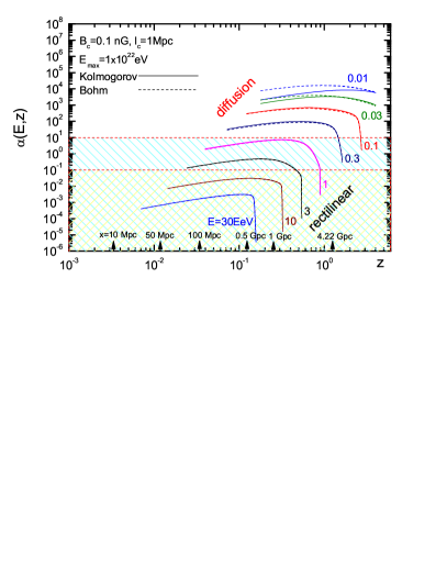
Figure 4: Parameter $\alpha(E,z)$ as a function of redshift $z$ for the magnetic field configuration $(B_{c},l_{c})=$ (0.1 nG, 1 Mpc). The observed energies in EeV are shown at the evolutionary curves. Parameter $\alpha$ changes along the particle energy trajectory $E_{g}={\mathcal{E}}(E,z)$. The mode of space propagation (diffusive, intermediate, rectilinear) is changing accordingly. The regions of propagation correspond to diffusion ($\alpha\geq 10$), rectilinear ($\alpha\leq 0.1$) and intermediate $(0.1\leq\alpha\leq 10)$. Along each trajectory the energy $E_{g}$ increases and $\alpha$ typically decreases due to increasing of $\lambda(E,E_{g})$.

As was explained in section 3, the various regimes of propagation are defined mostly by values of parameters $\alpha$, in particular, $\alpha\ll 1$ corresponds to rectilinear propagation and $\alpha\gg 1$ to diffusion. For the expanding universe $\alpha(E,t)$ is given by Eq. (39).

In Fig. 4 the evolution of $\alpha(E,z)$ is presented as function of redshift $z$, along the energy trajectories $E_{g}={\mathcal{E}}(E,z)$, where E is the observed energy. The evolution is shown for different $E$ and magnetic field configuration $(B_{c},l_{c})=$(0.1 nG, 1 Mpc).

Fig. 4 illustrates how protons with different observed energies $E$ propagate in different regimes (diffusive and rectilinear) and how the regimes are changing. The region with $\alpha\geq 10$ can be considered as diffusion, $\alpha\leq 0.1$ as rectilinear, and $0.1\leq\alpha\leq 10$ as intermediate. The protons with energy $E>1\times 10^{19}$ eV propagate only rectilinearly, $E\leq 3\times 10^{16}$ eV only diffusively, and with other energies – changing a regime of propagation. Equation for particle space density (42) takes into account automatically this changing of the propagation regimes.

6 Conclusion

Diffusion equations are intrinsically non-relativistic and superluminal velocities appear naturally there. The cardinal solution of this problem – the relativistic generalization of the diffusion equation – still expects to be found after more than 70 years of unsuccessful attempts.

The phenomenological approach in its most general form consists in transition of the diffusive regime to the rectilinear one in all cases where superluminal propagation appears. We study here this problem for diffusion of relativistic particles in magnetic fields. This transition has a problem: there is no extreme limit in which solution of diffusion equation, e.g. in the form of Eq. (7) or Eq. (35), obtains the form of rectilinear propagation. It requires an intermediate mode of propagation between two considered extreme regimes. This in principle follows from the numerical simulations. Diffusive regime is one where number of particles arriving from the different directions are equal with great precision and the resulting flux is given by $\vec{j}=-D\nabla n$. In the rectilinear propagation all particles arrive from the direction to a source. It is clear that in intermediate regime the particles are arriving from different direction with noticeable asymmetry which increases as energy rises, and analytic solution for such regime does not exists.

Although there is no way to obtain the rectilinear propagation as an extreme form of solution to diffusion equation, we do know that at high energy diffusion passes to rectilinear propagation. It follows from unlimited increase of $D(E)$ with $E$. For example, in the case of diffusion in turbulent magnetized plasma with maximum scale $l_{c}$,  $D(E)\propto E^{2}$ at $E>E_{c}$ (see section 2). Physically it is clear that very large diffusion coefficient means rectilinear propagation, but this argument says nothing about possibility of the formal transition of the diffusive solution to the rectilinear solution.

Our phenomenological approach for arbitrary mode of propagation is based on the definition of the propagator in the form of Eq. (13):

$$n(E,r)=\int_{0}^{\infty}dt\;Q[E_{g}(E,t),t]\;P(E,t,r)\;\frac{dE_{g}}{dE}(E,t),$$

where $n(E,r)$ is density of particles at distance $r$ from a source with the rate of particle generation $Q(E_{g})$. In principle the propagator $P(E,t,r)$ must be found as the Green function of the relativistic diffusion equation, but following the work (Dunkel et al., 2006) we found it from the mathematical analogy with the Maxwell distribution, given by Eqs. (11) and (12). Then the propagator $P(E,t,r)$ is found as relativistic Jüttner propagator, obtained for relativization of the Maxwell distribution, and expressed in the terms of diffusion variables (Dunkel et al., 2006). We generalized the parameters of the Jüttner distribution (19) to meet the more general requirements of particle propagation: arbitrary dependence of diffusion coefficient on energy and time and including the energy losses of the particles. We proved that our generalized Jüttner propagator $P_{gJ}(E,t,r)$ given by Eqs. (24) and (41) satisfies the following conditions:

• provides in all regimes velocities $v\leq c$,

• gives in extreme cases (in particular at low and high energies) the diffusive and rectilinear propagators,

• provides the normalized probability to find a particle in a unit volume at distance $r$ from a source at time $t$ after emission. Equality of this probability integrated over space to 1 guarantees the conservation of number of particles,

• gives the universal spectrum for homogeneous distribution of the sources, as it must be according to the propagation theorem (Aloisio & Berezinsky, 2004).

In other words, following in principle (Dunkel et al., 2006), we found the propagator $P_{gJ}(E,t,r)$ from the general requirements listed above, which include however as the main element the Jüttner propagator found from the mathematical analogy between the Maxwell non-relativistic distribution and diffusion equation (Dunkel et al., 2007). This strategy reminds the axiomatic approach to finding S-matrix in quantum theory, which is built on the basis of axioms without equations of propagation. Thus, the generalized Jüttner propagator gives much more than a simple interpolation between the diffusive and rectilinear regimes of propagation in magnetic fields. As one may see from the results, it successfully describes many features of the unified propagation and may be thought of as a reasonable approximation to the Green function of unknown fully relativistic equation for particle propagation, which includes the diffusion as a low-energy limit.

We have described in this paper the calculation of UHE proton fluxes in two cases. One is valid for propagation in stationary objects like e.g. galaxies and clusters of galaxies. This solution is described in section 3. The flux from a single source at a distance $r$ from an observer is given by Eq. (25) in terms of the new variable $\xi(t)$ and parameter $\alpha(E,\xi)$. The diffuse flux can be calculated by summation over the sources located in vertices of the space lattice with the source separation $d$.

The second case is given by propagation of UHE protons in the expanding universe. The diffuse flux is given by Eq. (49), where variable $\xi(t)$ and parameter $\alpha(E,t)$ are defined by the comoving length of a proton trajectory $\zeta(t)$ (see Eq. 39). In these calculations one does not need to take care of the propagation regime: it is selected automatically by values of $\xi$ and $\alpha$ in the process of integration.

7 Acknowledgments

We are grateful to Eugeny Babichev for discussions. This work is partially funded by the contract ASI-INAF I/088/06/0 for theoretical studies in High Energy Astrophysics.

References

- Aloisio et al. (2007) Aloisio, R. et al. 2007, Astropart. Phys., 27, 76
- Aloisio & Berezinsky (2004) Aloisio, R., & Berezinsky, V. 2004, ApJ, 612, 900
- Aloisio & Berezinsky (2005) Aloisio, R., & Berezinsky, V. 2005, ApJ, 625, 249
- Berezinsky et al. (1990) Berezinsky, V. S., Bulanov, S. V., Dogiel, V. A., Ginzburg, V. L., & Ptuskin, V. S. 1990, Astrophysics of Cosmic Rays, North-Holland
- Berezinsky & Gazizov (2006) Berezinsky, V., & Gazizov, A. Z. 2006, ApJ, 643, 8
- Berezinsky & Gazizov (2007) Berezinsky, V., & Gazizov, A. Z. 2007, ApJ, 669, 684
- Berezinsky, Gazizov & Grigorieva (2006) Berezinsky, V., Gazizov, A., & Grigorieva, S. 2006, Phys. Rev. D, 74, 043005
- Cubero et al. (2007) Cubero, D., Casado-Pascual, J., Dunkel, J., Talkner, P., & Hänggi, P. 2007, Phys. Rev. Lett., 99, 170601
- Dunkel et al. (2006) Dunkel, J., Talkner P., & Hänggi, P. 2006, arXiv:cond-mat/0608023v2
- Dunkel et al. (2007) Dunkel, J., Talkner, P., & Hänggi, P. 2007, Phys. Rev. D, 75, 043001
- Jüttner (1911) Jüttner, F. 1911, Ann. Phys. (Leipzig), 34, 856
- Landau & Lifshitz, v.10 (2001) Landau, L. D., & Lifshitz, E. M. 2001, Theoretcal Physics, vol. 10, Lifshitz, E. M., & Pitaevskii, L. P., Physics Kinetics, Fizmatlit
- Parizot (2004) Parizot, E. 2004, Nucl. Phys. B (Proc. Suppl.), 136, 169
- Syrovatsky (1959) Syrovatskii, S. I. 1959, Astron. Zh., 36, 17 [Astron. J., 3, 22]