Boundary conditions in local electrostatics algorithms

Abstract

We study the simulation of charged systems in the presence of general boundary conditions in a local Monte Carlo algorithm based on a constrained electric field. We firstly show how to implement constant-potential, Dirichlet, boundary conditions by introducing extra Monte Carlo moves to the algorithm. Secondly, we show the interest of the algorithm for studying systems which require anisotropic electrostatic boundary conditions for simulating planar geometries such as membranes.

I Introduction

In the simulation of condensed matter one very often imposes periodic boundary conditions in order to minimize surface artefacts which give rise to slow convergence of energies to their bulk values. While such boundary conditions are simple to understand for short-ranged potentials they lead to many subtleties when working with charged systems de Leeuw et al. (1980); Fraser et al. (1996). Attempts at simplifying the problem by using truncated potentials lead to violations of basic sum rules on the structure factor Stillinger and Lovett (1968), incorrect number fluctuations in finite systems Lebowitz (1983) or even loss of electrical conductivity Marchetti and Kirkpatrick (1985). The correct treatment of charged media requires a full treatment of the long-ranged Coulomb interaction.

Classical methods of treating the Coulomb interaction use careful mathematical analysis to convert the conditionally convergent Coulomb sum into a well defined mathematical object such as the Ewald sum de Leeuw et al. (1980). Recently we introduced an alternative treatment of the Coulomb problem that allows one to replace the global calculation of the interaction energy by a local dynamic process Maggs and Rossetto (2002); Maggs (2002); Levrel et al. (2005). The main interest in this transformation is that it enables one to perform a local Monte Carlo simulation in the presence of charges and dielectrics, without ever solving the Poisson equation. The algorithm works by evolving the electric field in time (in a manner similar to Maxwell’s equations) while eliminating “uninteresting” degrees of freedom such as the magnetic field. The algorithm uses the energy

$$U=\int\frac{\epsilon_{0}\mathbf{E}^{2}}{2}\>\mathrm{d}{{}^{3}}r$$ (1)

where $\mathbf{E}$ is the electric field while implementing Gauss’ law

$$\epsilon_{0}\nabla\cdot\mathbf{E}-\rho=0$$ (2)

as a dynamic constraint. We showed Maggs (2004) that the algorithm can be used to generate tin-foil or vacuum boundary conditions if one chooses appropriate dynamics for the $\mathbf{q}=0$ component of the electric field. Until now applications have been to the properties of bulk, three dimensional media Pasichnyk and Dünweg (2004); Rottler and Maggs (2004a) in periodic systems.

This paper generalizes the method to a broader class of physical systems and boundary conditions. Firstly we consider the case, particularly important in devices and electrodes, of imposition of an external potential on a metallic surface; a case which requires the use of Dirichlet boundary conditions for the potential. Again we find that the locality of the formulation allows the simulation of a broader class of geometries, including those for which the use of fast Fourier techniques is difficult.

A second generalization of the method is required to treat anisotropic systems, in particular membranes. The simulation of thin, quasi two-dimensional systems in three-dimensional space is surprisingly difficult Yeh and Berkowitz (1999); Arnold and Holm (2002); Arnold et al. (2002). The use of a purely local algorithm requires only small modifications in order to minimize finite size effects; we argue that it will also give rather favorable complexity in the limit of large number of particles, $N$.

Our paper contains two, independent, self-contained theoretical sections. Firstly in II we treat the problem of metallic boundary conditions including certain subtleties as to how a true metal behaves. Secondly in III we consider electrostatics in anisotropic $2+1$ dimensional geometries. Implementation of the ideas has been performed by Thompson and Rottler Thompson and Rottler (2008) using off lattice techniques suitable for atomistic simulation. In their paper they compare detailed simulations with available theories.

II Metallic boundary conditions

We begin by emphasizing the difference between idealized metallic boundaries and true physical systems in which screening occurs over a small but finite Debye length. We then show how to impose Dirichlet conditions on the potential, $\phi$ while still keeping $\mathbf{E}$ as the main dynamic variable.

The nature of metallic boundary conditions

There are two different, self-consistent ways of calculating the energy of charges in the presence of a dielectric or conducting interfaces. In the first treatment we calculate the potential energy arising from the solution of the Poisson equation

$$\nabla\cdot(\epsilon\nabla\phi)=-\rho$$

with $\rho$ the density of free charges, with the appropriate boundary conditions for each configuration. The boundary condition at a metallic surface is that the tangential electric field vanishes, while the normal field at the surface satisfies

$$\mathbf{D}\cdot\mathbf{n}=\epsilon\mathbf{E}\cdot\mathbf{n}=-\sigma$$ (3)

where $\sigma$ is the surface charge density. The field is identically zero within a conductor Landau et al. (1998). The internal energy is then

$$U=\frac{1}{2}\int\phi\rho\>\mathrm{d}{{}^{3}}r.$$ (4)

In this case the longitudinal electric field is static, and is given by $\mathbf{E}=-\nabla\phi$. We note that in this treatment thermal fluctuations play no role so that certain fluctuation phenomena such as thermal Casimir interactions are neglected.

A physical system at a non-zero temperature always presents polarization or charge fluctuations; superposed on the interaction energy Eq. (4) is an effective potential coming from these fluctuations. We now work in the Debye–Hückel limit to calculate an approximate correlation function for the electric field in a conducting system at finite temperatures. This illustrative calculation shows that transverse field fluctuations become important as soon as the temperature $T>0$.

We consider a one component plasma, with neutralizing background. We approximate the free energy of a conductor as a sum of the electric field energy Eq. (1) and the configurational entropy of the charges with the functional Maggs (2004)

$$F=\int\left\{\frac{\epsilon_{0}\mathbf{E}^{2}}{2}+k_{B}T\;c\ln{c}\right\}\>\mathrm{d}{{}^{3}}r$$ (5)

where $c(\mathbf{r})=\rho(\mathbf{r})/e$ is the number density of mobile ions and $e$ the charge of the particles. In the limit of small fluctuations of density $\delta c(\mathbf{r})$ we expand to second order and use charge conservation so that $\int\delta c\>\mathrm{d}{{}^{3}}r=0$. Then

$$F(\delta c,\mathbf{E})=\int\left\{\frac{\epsilon_{0}\mathbf{E}^{2}}{2}+k_{B}T\;\frac{(\delta c)^{2}}{2c_{0}}\right\}\>\mathrm{d}{{}^{3}}r$$

where $c_{0}$ is the mean background density of the ions. We now eliminate the charge fluctuation with the help of Gauss’ law and find an effective action for the electric field

$$F_{E}=\int\epsilon_{0}\left\{\frac{\mathbf{E}^{2}}{2}+\frac{(\nabla\cdot\mathbf{E})^{2}}{2\kappa^{2}}\right\}\>\mathrm{d}{{}^{3}}r$$ (6)

with $\kappa$ the inverse Debye length. From Eq. (6) we read off the longitudinal and transverse correlations of the electric field,

$$\epsilon_{0}\langle\mathbf{E}(q)\mathbf{E}(q)\rangle_{long} =\frac{k_{B}T}{1+q^{2}/\kappa^{2}},$$

$$\epsilon_{0}\langle\mathbf{E}(q)\mathbf{E}(q)\rangle_{tran} =k_{B}T.$$

On wavelengths large compared with the screening length ($q/\kappa<<1$) all longitudinal and transverse electric modes fluctuate with the same amplitude.

It is instructive to compare with similar calculations for an explicit model of dielectric in terms of polarization fluctuations Maggs and Everaers (2006). We find that

$$\epsilon_{0}\langle\mathbf{E}(q)\mathbf{E}(q)\rangle_{long} =k_{B}T\;\frac{\epsilon-\epsilon_{0}}{\epsilon},$$

$$\epsilon_{0}\langle\mathbf{E}(q)\mathbf{E}(q)\rangle_{tran} =k_{B}T.$$

Again transverse field correlations are unchanged in the presence of a dielectric or classical charged fluid, longitudinal fluctuations depend on the material properties. In the limit $\epsilon\rightarrow\infty$ the fluctuations of a dielectric are the same as those of a metal for $q\ll\kappa$.

From these expressions in Fourier space we calculate the correlations of the electric field in real space. For a dielectric (with $\epsilon<\infty$) we find that the field displays dipolar correlations so that

$$\langle E_{i}(\mathbf{r})E_{j}(\mathbf{r}^{\prime})\rangle\sim\frac{1}{|\mathbf{r}-\mathbf{r}^{\prime}|^{3}},$$

field correlations are long-ranged. This dipolar correlation in the fields leads to long-ranged Casimir/Lifshitz interactions between dielectrics. For a conducting system field correlations decay exponentially with characteristic length the Debye length,

$$\langle E_{i}(\mathbf{r})E_{j}(\mathbf{r}^{\prime})\rangle\sim e^{-\kappa|\mathbf{r}-\mathbf{r}^{\prime}|}.$$

From these considerations we see that different strategies are needed to simulate the idealized classical metallic boundary condition Eq. (3) or a true fluctuating charged fluid. In the first situation one only needs information on the fields in the nonconducting regions. In the second case the surface field is influenced by fluctuations that occur within a few Debye lengths of the surface. The surface must then be simulated explicitly with an expression such as Eq. (5) in order to obtain results including Casimir/Lifshitz type interactions. We note that such interactions are very weak on the macroscopic scale. Between two plates of area $A$ separated by a distance $H$ the thermal interactions are given by Kardar and Golestanian (1999)

$${U}=-Ak_{B}T\frac{\zeta(3)}{16\pi H^{2}}$$

with $\zeta(3)\approx 1.20$

In this paper we will only consider the case of imposing the first type of metallic boundary conditions in which fluctuation forces are neglected.

Fixed-potential boundary conditions

Minimization principle

We now apply our local simulation algorithm to fixed-potential boundary conditions of the type Eq. (3). The method of attack is a generalization of the methods of Ref. Maggs and Rossetto, 2002. Firstly we seek a variational principle for the electric field for which the energy is a true minimum for the geometry of interest. We then promote the constraints of the minimization principle to $\delta$-functions in a partition function. This partition function is then shown to generate the same relative statistical weights as the original variational energy, but is much more convenient for the purposes of simulation since it allows the local update of fields in a Monte Carlo algorithm.

As noted in the introduction electrostatic interaction is calculated by minimizing the electric field energy Eq. (1) in the presence of the constraint of Gauss’ law, Eq. (2), using the functional

$$A[\mathbf{E}]=\int\left[\frac{\epsilon_{0}\mathbf{E}^{2}}{2}+\lambda(\epsilon_{0}\nabla\cdot\mathbf{E}-\rho)\right]\>\mathrm{d}{{}^{3}}r,$$

where $\lambda$ is a Lagrange multiplier. We now generalize Ref. Schwinger et al., 1998 and consider a system with both free charges and conductors, $i$. These conductors are maintained by external sources at fixed potentials $\phi^{\text{(ext)}}_{i}$. This is most conveniently done by performing Legendre transform Landau et al. (1998) in order to eliminate for the unknown surface charge densities $\sigma=\{\sigma_{i}\}$ on the surfaces $S=\{S_{i}\}$ in order to replace them by the potentials $\phi^{\text{(ext)}}=\{\phi^{\text{(ext)}}_{i}\}$:

$$U_{2}[\mathbf{E},\sigma]=U[\mathbf{E}]-\oint\sigma\phi^{\text{(ext)}}\mathrm{d}S.$$ (7)

We now impose the boundary condition Eq. (3) with a further Lagrange multiplier $\mu$ living on each surface and consider the functional

$$A_{2}=U_{2}+\int\lambda(\epsilon_{0}\nabla\cdot\mathbf{E}-\rho)\>\mathrm{d}{{}^{3}}r+\oint\mu(\epsilon_{0}\mathbf{n}\cdot\mathbf{E}+\sigma)\;\mathrm{d}S.$$ (8)

In order to find the stationary point of $A_{2}$ we vary all the fields, and integrate by parts using $\lambda\nabla\cdot\delta\mathbf{E}=\nabla\cdot(\lambda\delta\mathbf{E})-(\nabla\lambda)\cdot\delta\mathbf{E}$ and find

$$\delta A_{2}=\int[\epsilon_{0}\;\delta\mathbf{E}\cdot(\mathbf{E}-\nabla\lambda)+\delta\lambda\;(\epsilon_{0}\nabla\cdot\mathbf{E}-\rho)]\>\mathrm{d}{{}^{3}}r\\ -\oint[\delta\sigma(\phi^{\text{(ext)}}+\mu)+\delta\mu(\epsilon_{0}\mathbf{n}\cdot\mathbf{E}+\sigma)-\epsilon_{0}(\lambda-\mu)\delta\mathbf{E}\cdot\mathbf{n}]\;\mathrm{d}S.$$

At the stationary point we find

$$\delta\mathbf{E} :\quad\left\{\begin{aligned} &\mathbf{E}-\nabla\lambda=0\\ &\lambda-\mu=0\end{aligned}\right. \begin{aligned} &\text{in $V$,}\\ &\text{on $S$,}\end{aligned}$$

$$\delta\sigma :\quad\phi^{\text{(ext)}}+\mu=0 S$$  on ,

$$\delta\lambda :\quad\epsilon_{0}\nabla\cdot\mathbf{E}-\rho=0 V$$  in ,

$$\delta\mu :\quad\epsilon_{0}\mathbf{n}\cdot\mathbf{E}+\sigma=0 S$$  on .

The first equation implies that $\mathbf{E}$ is the gradient of a potential, $\phi=-\lambda$. The next two imply that $\phi=\phi^{\text{(ext)}}$ on $S$ so that we indeed generate Dirichlet conditions. Finally the last two equations impose Gauss’ law. At the stationary point thus we have $\mathbf{E}=\mathbf{E}_{p}=-\nabla\phi_{p}$ and $\sigma=\sigma_{p}$, where the index $p$ signals the solution to Poisson’s equation with Dirichlet boundary conditions.

Partition function

We now generalize the stationary principle to finite temperatures and replace the Lagrange multipliers of Eq. (8) by $\delta$-functions in a functional integral. Let us define a partial partition function, where the bulk charge distribution $\rho$ is given, as

$$Z_{\rho}=\int\mathcal{D}\mathbf{E}\ \mathcal{D}\sigma\;\delta(\epsilon_{0}\nabla\cdot\mathbf{E}-\rho)\>\delta(\epsilon_{0}\mathbf{n}\cdot\mathbf{E}+\sigma)\>\mathrm{e}^{-\beta U_{2}[\mathbf{E},\sigma]}.$$ (9)

We integrate over the electric field, constrained by Gauss’ law and also all values of the surface charge $\sigma$ compatible with the flux condition at the surface of the conductors.

The full partition function is calculated by integrating over the position of all mobile charges. In order to find the interaction in terms of the minimum of the functional it is convenient to change integration variables so that $\mathbf{E}=\mathbf{E}_{p}+\mathbf{e}$ and $\sigma=\sigma_{p}+s$. After noting that $\sigma_{p}=-\epsilon_{0}\mathbf{n}\cdot\mathbf{E}_{p}$ we find

$$Z_{\rho} =\int\mathcal{D}\mathbf{e}\ \mathcal{D}s\;\delta(\nabla\cdot\mathbf{e})\>\delta(\epsilon_{0}\mathbf{n}\cdot\mathbf{e}+s)$$

$$\times\qquad\mathrm{e}^{-\beta\left[\int\frac{\epsilon_{0}}{2}(\mathbf{E}_{p}+\mathbf{e})^{2}\>\mathrm{d}{{}^{3}}r-\oint(\sigma_{p}+s)\phi^{\text{(ext)}}\>\mathrm{d}S\right]}.$$

With the help of the constraint equations we find

$$Z_{\rho} = \mathrm{e}^{-\beta U_{2}[\mathbf{E}_{p},\sigma_{p}]}$$

$$\times \int\mathcal{D}\mathbf{e}\ \mathcal{D}s\;\delta(\nabla\cdot\mathbf{e})\>\delta(\epsilon_{0}\mathbf{n}\cdot\mathbf{e}+s)\>\mathrm{e}^{-\beta U_{2}[\mathbf{e},s]}$$

so that

$$Z_{\rho}=\mathrm{e}^{-\beta U_{2}[\mathbf{E}_{p},\sigma_{p}]}\>{Z}_{\text{fluct}},$$ (10)

with ${Z}_{\text{fluct}}$ independent of positions of the mobile charges. This results in a complete factorization of the statistical weights of charge configurations and of field and surface charge fluctuations

$$Z=\biggl{[}\int\Bigl{(}\prod_{j}\>\mathrm{d}{{}^{3}}r_{j}\Bigr{)}\mathrm{e}^{-\beta U_{2}[\mathbf{E}_{p},\sigma_{p}]}\biggr{]}{Z}_{\text{fluct}}={Z}_{\text{Coulomb}}{Z}_{\text{fluct}}.$$

We note, however, that following the discussion of Section II, this fluctuation partition function is not necessarily the true physical fluctuation partition function that one would calculate for a true physical metal. Thus sampling with the partition function Eq. (9) will not necessarily give the correct fluctuation forces acting on electrodes even if, by construction, it generates the correct relative weight for configurations of free charges.

Algorithm

The result Eq. (10) is the analytical basis for an algorithm that simulates fixed-potential surfaces. Sampling the partition function requires updates generating fluctuations of the variables, $\{\mathbf{r}_{j}\}$, $\mathbf{E}$ and $\sigma$. We refer the reader to previous work Maggs and Rossetto (2002); Levrel et al. (2005); Levrel and Maggs (2005) for particle updates and bulk field updates. We note that the demonstration requires an integral over the surface charge $\sigma$; thus even if charges in the volume are discrete those on surfaces should be sampled continuously.

In order to sample the partition function Eq. (9) two new moves need to be introduced. Firstly, fluctuation in the charge density in the surface of a given conductor that conserve its total charge. This move is implemented by a variation of the simplest update for volume charges. A random charge amplitude $\delta$ is generated to make a charge pair of $+\delta$ at one site and $-\delta$ at a second site. Since field lines must lie outside the conductor, Fig. 1, we update the field on three links connecting the modified sites. To sample the integral Eq. (9) the charges should be chosen from a continuum distribution. Secondly, each conductor $i$ bears a net charge $\int_{S_{i}}\sigma_{i}$ which should also fluctuate. This is achieved by transferring charges between pairs of conductors. Gauss’ law then requires modifying the total electric flux between the two surfaces.

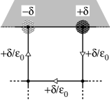
Figure 1: Local update for integrating surface charge fluctuations. Grey region represents the conductor volume (where $\mathbf{E}=0$); the white region is the dielectric.

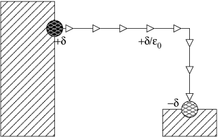
Figure 2: Updating the total charge of conductors implies updating the field along a line connecting them. This update is not local.

We now demonstrate that despite the need to transfer charge large distances between conductors this does not dominate the time need to simulate the system. We start by noting that fluctuations on a conductor can be estimated using an argument based on the capacitance of an isolated conductor Jancovici (2003). In three dimensions the capacitance of an object of size $d$ scales as $C=\epsilon_{0}d$. If we equate the charging energy to the thermal energy scale we find

$$k_{B}T=\frac{Q^{2}}{2C}\sim\frac{Q^{2}}{\epsilon_{0}d}$$

so that the amplitude of charge fluctuation of a conductor is $Q^{2}\sim k_{B}T\epsilon_{0}d$. Consider a Monte Carlo trial in which a charge $\delta$ is sent along a path of length $\ell$, Fig. 2. Then Levrel and Maggs (2005) we estimate the energy change as $\ell\delta^{2}/\epsilon_{0}a^{2}$, with $a$ the mesh spacing. For this trial to be successful we again require that this energy is matched to the thermal fluctuations giving $\delta^{2}\sim\epsilon_{0}a^{2}k_{B}T/\ell$. Thus the amplitude of the charge transfer over large distances must be small.

We now consider $M$ such exchanges. Since charges are transferred in each direction we require that $M\delta^{2}=Q^{2}$, or $M\sim\ell d/a^{2}$. Each transfer requires a numerical effort that is also $O(\ell/a)$ to update the links so that a total computational effort ${\eta}=\ell^{2}d/a^{3}$ is needed to equilibrate the charge fluctuations between the conductors. In any practical simulation in a box of dimension $L$ we expect that ${\eta}<L^{3}/a^{3}$, so that the effort need to equilibrate charges between conductors is less than that required to perform a single sweep of the bulk of the simulation.

We thus have the basis for the generalization of a local Monte Carlo algorithm for simulating charges in the presence of Dirichlet boundary conditions. Conventional methods for treating this problem use fast Fourier techniques in simple separable geometries, such as regular simulation cells. The use of a local formulation of the electrostatics allows one to implement such boundary conditions in arbitrary geometries — including rough surfaces or irregular electrodes where Fourier analysis does not work.

III Simulating systems with slab geometries

We now pass to consideration of a second important class of boundary conditions that should be imposed in the study of systems with planar geometries. Examples include thin quasi two-dimensional slabs isolated in three-dimensional space, or in the biophysical field simulation of proteins in a lipid membrane with an implicit solvent. In order to generate the correct Coulomb interactions between particles with grid based methods the thin sample must be embedded in a thick three-dimensional simulation box. This box then contains many more degrees of freedom than the original particle system. For reasons of efficiency one wishes to make the repeat distance perpendicular to the thin sample as small as possible, however if this repeat distance is too small multiple copies of the sheet “see” each other and introduce artefacts in the simulation.

Imposition of tin-foil or vacuum boundary conditions gives rise to simulations that converge very slowly as the system size is increased. The crucial insight into how to accelerate this convergence was provided in Ref. Yeh and Berkowitz, 1999 and efficient implementations are now available that translate these ideas Arnold et al. (2002); de Joannis et al. (2002) in molecular dynamics. Our aim here is to reproduce this rapid convergence in a local formulation of electrostatics, and to argue that the asymptotic complexity is at least as good as $N^{3/2}$ and in many systems $N^{1}$.

In standard approaches to the electrostatic energy all the complexity comes from the transformation from an ambiguous, conditionally convergent sum (a sum whose answer depends on the order of evaluation) into a rapidly converging, unambiguous expression, such as the Ewald formula de Leeuw et al. (1980). In local formulations there is no equivalent to the conditional convergence. Instead one is left with different, inequivalent, choices for the treatment of the zero wavevector component of the electric field $\mathbf{E}(q=0)$ Maggs (2004). Let us first review the origin of these different choices.

Periodic boundary conditions in local algorithms

In periodic boundary conditions an arbitrary vector field can be decomposed into three terms

$$\mathbf{E}=-\nabla\phi+\nabla\times\mathbf{G}+\bar{\mathbf{E}}$$

where the potential $\phi$ is periodic, as is $\mathbf{G}$. $\bar{\mathbf{E}}$ is a constant; it is the zero wavevector component of the electric field, $\mathbf{E}(q=0)$. With this decomposition the energy is given by the sum of three independent terms

$$U=\frac{\epsilon_{0}}{2}\left\{\int(\nabla\phi)^{2}\>\mathrm{d}{{}^{3}}r+\int(\nabla\times\mathbf{G})^{2}\>\mathrm{d}{{}^{3}}r+V\>\bar{\mathbf{E}}^{2}\right\}$$

with $V$ the volume of the simulation cell. Cross-terms are shown to be zero on integration by parts. The simplest version of the local Monte Carlo algorithm uses two updates Maggs and Rossetto (2002).

• Motion of charges $q$ along links $l$ together with a slaved update of the electric field on the link according to $E_{l}\rightarrow E_{l}-q/\epsilon_{0}$. Both the longitudinal and transverse components of the field are modified, as well as the $q=0$ component, $\bar{\mathbf{E}}$.

• A plaquette update which leaves unchanged both $\bar{\mathbf{E}}$ and the longitudinal field $-\nabla\phi$, modifying only $\mathbf{G}$.

This pair of updates are respectively a discretized analog of the two terms on the right hand side of the Maxwell equation

$$\epsilon_{0}\frac{\partial\mathbf{E}}{\partial t}=-\mathbf{J}+\nabla\times\mathbf{H}.$$

Integrating the Maxwell equation over both time and the simulation volume we see that the $q=0$ component of the field and the dipole moment of the system of charges $\mathbf{d}=\int\!\!\mathrm{d}t\int\!\!\>\mathrm{d}{{}^{3}}r\mathbf{J}$ are linked by $\epsilon_{0}V\bar{\mathbf{E}}+\mathbf{d}=\mathrm{const}$, a conservation law which remains valid for the discretized equations.

Thus the simplest form of the algorithm samples the partition function

$$Z=\int\mathcal{D}\mathbf{E}\;\delta(\nabla\cdot\mathbf{E}-\rho)\>\delta(\epsilon_{0}V\bar{\mathbf{E}}+\mathbf{d})\>e^{-\beta\int\epsilon_{0}\mathbf{E}^{2}/2\>\mathrm{d}{{}^{3}}r}.$$ (11)

If we introduce the solution to the Poisson equation in periodic boundary conditions $\phi_{p}$ then we see that this partition function samples configurations with the effective energy

$$U_{\mathit{eff}}=\int\frac{\epsilon_{0}(\nabla\phi_{p})^{2}}{2}\>\mathrm{d}{{}^{3}}r+\frac{\mathbf{d}^{2}}{2\epsilon_{0}V}.$$ (12)

This result is very similar to that found using careful evaluation of the Coulomb sum de Leeuw et al. (1980) which gives

$$U_{lps}=\int\frac{\epsilon_{0}(\nabla\phi_{p})^{2}}{2}\>\mathrm{d}{{}^{3}}r+\frac{\mathbf{p}^{2}}{2(1+2\epsilon_{s})\epsilon_{0}V}$$

where $\mathbf{p}$ is the cell dipole moment and $\epsilon_{s}$ the relative dielectric constant of an “exterior” reference medium, two common choices being $\epsilon_{s}=1$ for vacuum boundary conditions and $\epsilon_{s}=\infty$ for metallic or tin-foil boundary conditions. The expression resulting from the local algorithm is very similar to that found in the summation method if we take $\epsilon_{s}=0$ and we notice that $\mathbf{d}$ and $\mathbf{p}$ are almost identical. $\mathbf{p}$ is the dipole moment of the charge images inside the Bravais cell being used in the simulation; when a particle crosses the boundary of the cell it is replaced by that of its periodic images which enters the cell so that $\mathbf{p}$ is discontinuous. $\mathbf{d}$ is a dipole moment which is continuous on crossing Bravais cell boundaries, thus it keeps track of how many times the particles wind around the simulation box:

$$\mathbf{p}=\mathbf{d}-\sum_{i}\mathbf{a}_{i}q_{i}$$

where $q_{i}$ is the charge of each particle in the simulation cell and $\mathbf{a}_{i}$ is a Bravais lattice vector.

The authors of Ref. Levrel et al., 2005 introduced another update scheme for the electric field based on a worm algorithm widely used in the simulation of quantum spins Alet and Sørensen (2004). The algorithm nucleates a pair of virtual charges $\pm q_{v}$. One of these charges diffuses until it returns to its companion where the two charges annihilate. If the mobile charge is confined to the periodic cell then during the move only the transverse field $\nabla\times\mathbf{G}$ is updated. If the particle is allowed to wind around the cell it breaks the conservation law on $\epsilon_{0}V\bar{\mathbf{E}}+\mathbf{d}$, removing the second $\delta$-function in Eq. (11). We then find that the effective energy Eq. (12) is independent of $\mathbf{d}$; we have effectively periodic, that is tin-foil, boundary conditions. A similar result is found by including $\bar{\mathbf{E}}$ as a single extra dynamic variable which must be updated with a third, independent Monte Carlo move Maggs and Rossetto (2002); Rottler and Maggs (2004b).

Finite size effects in slab geometries

We now give a short argument for the slow convergence of the interaction energy for systems which are simulated in slab geometries. Rigorous calculations which provide the full justification are to be found in the literature Fraser et al. (1996); Yeh and Berkowitz (1999); Arnold et al. (2002). Consider a thin, quasi two-dimensional system embedded in a simulation box of dimensions $L^{2}\times L_{z}$; usually one is interested in the case $L_{z}/L>1$ so that successive periodic images do not interact too strongly.

The slow convergence of the energy can be understood by considering the electrostatic potential in a mixed real-space/Fourier representation, $\hat{\phi}(\mathbf{q}_{\parallel},z)$ where $\mathbf{q}_{\parallel}$ denotes the transverse wavevector in the $(x,y)$ plane. Using the fact that polarization of a sample is equivalent to a space charge $\rho=-\nabla\cdot\mathbf{P}$ the mean polarization of the thin sample in the $z$ direction is equivalent to two charge sheets of strength $\sigma=\pm p_{z}/L^{2}h$ where $p_{z}$ is the $z$ component of the dipole moment and $h$ the sample thickness. The interesting physics occurs in the equation for $q_{\parallel}=0$. We consider a single cell in the $z$ direction, placing the source $-\sigma$ at $z=0$ and the second $+\sigma$ at $z=h$. Then

$$\epsilon_{0}\frac{\partial^{2}\hat{\phi}(0,z)}{\partial z^{2}}=\sigma\left[\delta(z)-\delta(z-h)\right].$$

This has as a solution

$$\hat{\phi}(0,z) =(-e_{0}+\sigma/\epsilon_{0})z 0 <z<h$$

$$=(-e_{0}+\sigma/\epsilon_{0})h-e_{0}(z-h) h <z<L_{z}$$

where we have used continuity, but not periodicity, of the potential. $e_{0}$ is a yet to be determined integration constant; it corresponds to the electric field flowing between two copies of the simulation cell, Fig. 3. The $z$ component of the electric field is

$$E_{z} =E^{int}=e_{0}-\sigma/\epsilon_{0}\quad 0 <z<h$$

$$=E^{ext}=e_{0}\quad h <z<L.$$

The energy of this simulation cell is the integral of $\epsilon_{0}E_{z}^{2}/2$,

$$U_{\mathit{Coulomb}}=\frac{\epsilon_{0}L^{2}}{2}\left\{(e_{0}-\sigma/\epsilon_{0})^{2}h+(L_{z}-h)e_{0}^{2}\right\}.$$

The classical tin-foil solution is recovered by setting $e_{0}=\sigma h/\epsilon_{0}L_{z}$ so that the potential is periodic, $\phi(0)=\phi(L_{z})$, Fig. 3, and the average field $\bar{E}_{z}=\frac{1}{L_{z}}\int\mathrm{d}z\,E_{z}(z)=0$. But the energy then depends on $L_{z}$,

$$U_{\mathit{Coulomb}}=U_{\infty}-\frac{p_{z}^{2}}{2\epsilon_{0}L^{2}L_{z}}$$ (13)

where $U_{\infty}$ is the energy in the limit of large $L_{z}$. If one considers a series of slabs with identical dipole moment and transverse dimensions and vary $L_{z}$ then the energy converges as only $1/L_{z}$; very large, and mostly empty boxes must be simulated in order to reduce finite size artefacts.

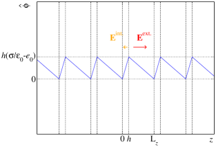
Figure 3: Plot of $\hat{\phi}(0,z)$ in the presence of a double layer. $E^{int}=e_{0}-\sigma/\epsilon_{0}$, $E^{ext}=e_{0}$, with $e_{0}=\sigma h/\epsilon_{0}L_{z}$. Potential plotted over several simulation cells. The non-zero $E^{ext}$ couples successive periodic images.

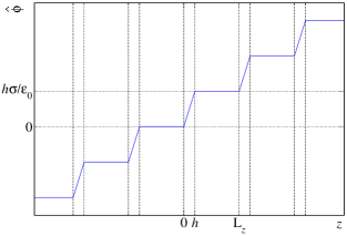
Figure 4: Plot of $\hat{\phi}$ with $e_{0}=0$. The field between slabs, $E^{ext}$, is zero. There is no dipolar interaction between the slabs.

There is no such convergence problem when using anisotropic electrostatic boundary conditions in which the exterior field is always zero: $e_{0}=0$, Fig. 4. The energy is $U_{\mathit{Coulomb}}=U_{\infty}$, independent of $L_{z}$. The local algorithm automatically gives $e_{0}=0$, as do Maxwell’s equations; in order to still have $\bar{E}_{x}=\bar{E}_{y}=0$ we require tin-foil boundary conditions in the $(x,y)$ plane. Our method implicitly includes the $+p_{z}^{2}/2\epsilon_{0}V$ correction that potential-based algorithms need to add to the tin-foil energy. Since the particles remain confined to a single lattice cell in the $z$ direction there is no distinction between $d_{z}$ and $p_{z}$.

Let us now consider the effect of density fluctuations with the plane, by studying the Poisson equation for wavevectors $\mathbf{q}_{\parallel}\neq 0$:

$$-q_{\parallel}{}^{2}\hat{\phi}+\frac{\partial^{2}\hat{\phi}}{\partial z^{2}}=-\frac{{\hat{\rho}(\mathbf{q}_{\parallel},z)}}{\epsilon_{0}}.$$

Outside of the slab where $\hat{\rho}=0$ we conclude that

$$\hat{\phi}(\mathbf{q}_{\parallel}\neq 0,z>h)\sim\mathrm{e}^{\pm q_{\parallel}z}$$

where $\mathbf{q}_{\parallel}=0$ corresponds to the special case treated above. The next longest-ranged component to the interaction must come from modes of the form $(2\pi/L,0,0)$ and lead to interactions decaying as $\mathrm{e}^{-2\pi L_{z}/L}$. Already when $L_{z}/L=3$ one finds a reduction in the interaction by a factor $7\times 10^{-9}$.

Numerical tests

To test these ideas we simulated a lattice gas with a slab geometry using the local algorithm. The lattice spacing $a$ is set to unity. We start a simulation with all positive and negative charges superposed at $z=0$ and $\mathbf{E}=0$ in the whole simulation volume. We then displaced positive charges to $z=1$, creating a dipolar sheet, updating the fields according to the constrained algorithm. We simulated the fields using several different temperatures, $T$ and cell heights, $L_{z}$. The total energy can be decomposed into a static, electrostatic contribution plus a thermal energy $N_{pl}k_{B}T/2$ coming from equipartition in the $N_{pl}$ degrees of freedom associated with the transverse excitations. On fitting the total energy to the form

$$\langle U\rangle=U_{\mathit{Coulomb}}(L_{z})+\frac{k_{B}TN_{pl}}{2}$$

we extracted an estimate of the electrostatic energy as a function of the cell dimensions.

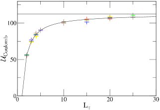
Figure 5: Electrostatic energy of the slab system when all three components of $\bar{\mathbf{E}}$ are sampled independently, corresponding to tin-foil boundary conditions. Simulation results (+) follow Eq. (13). $L=15$, $\epsilon_{0}=1$. Five values of $k_{B}T$ from $0.1$ to $0.5$ for each $L_{z}$.

In a first series of simulations we imposed the equivalent of tin-foil boundary conditions by including the three components of $\bar{\mathbf{E}}$ in the set of dynamic fields. The results are shown in Fig. 5; as a guide to the eye we added the continuous curve which corresponds to a correction in the energy varying as $1/L_{z}$ (with the analytically determined prefactor). In a second series of simulations updates to $\bar{E}_{z}$ are dropped. Fig. 6 shows that the electrostatic energy is now independent of $L_{z}$ to within the precision of the measurements and equal to $U_{\infty}$. The natural coupling between $\mathbf{d}$ and $\bar{\mathbf{E}}$ introduced by our local method removes the dipolar interaction between replicas of the slab.

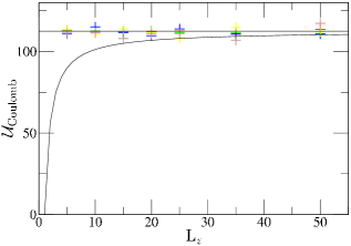
Figure 6: Coulomb energy of the slab system when $\bar{E}_{z}$ is not updated independently of charges. Simulation results (+) are independent of $L_{z}$. $L=15$, $\epsilon_{0}=1$. Five values of $k_{B}T$ from $0.1$ to $0.5$ for each $L_{z}$.

Discussion

In a local Monte Carlo simulation the most obvious implementation would use a mixture of local updates of the particles together with the worm algorithm Levrel et al. (2005); Alet and Sørensen (2004) in order to integrate over the transverse degrees of freedom in the empty bulk of the simulation. This worm algorithm re-equilibrates the transverse field with an effort which is $O(1)$ per updated degree of freedom (which corresponds to plaquettes). If one were to use just a single worm update per sweep of the particles then we find a complexity per sweep which varies as $O(N)$ for the particle motion, and $O(N^{3/2})$ for the worm dynamics. In practice launching a worm which simulates the entire simulation box for every particle sweep results in an oversampling of the uninteresting transverse degrees of freedom. If one simulates a set of particles for a time $\tau$ then diffusion motion in the plane will give a typical displacement $\ell_{t}\sim\sqrt{\tau}$. A worm which updates plaquettes a distance more than $\ell_{t}$ from the slab is doing unnecessary work.

This suggests the following hierarchical scheme: every sweep we launch a worm confined to the simulation slab thickness $h$, then every $4$ sweeps we launch a worm confined to a distance $2h$. Similarly every $2^{2n}$ sweeps we allow the worm to propagate $2^{n}h$ in the $z$ direction. In such a scheme the longest wavelength modes of the electric field are re-equilibrated on the same timescale as is needed for particles to diffuse across the simulation box. The worm then spends most of its time updating at the scale of the slab so that the total algorithm has a complexity scaling as $N^{1}$.

IV Conclusion

We have considered the formulation of generalized boundary conditions in a form useful for local electrostatic simulation algorithms. We have shown how to treat metallic boundaries for which one imposes a constant potential at a surface. An additional Monte Carlo move which transfers charge between conductors performs the Legendre transformation from a constant-charge to a constant-potential ensemble.

The local algorithm (like Maxwell’s equations) naturally generates a dipolar contribution to the solution to the Poisson equation in a periodic simulation cell. By choosing an anisotropic integration over the $q=0$ components of the electric field we reduce the spurious interaction between different copies of a planar system.

Molecular dynamics implementations of both problems are potentially possible Rottler (2007). For the first problem of constant-potential simulation one could alternate between a symplectic integrator (e.g. velocity Verlet) for the particles and a Monte Carlo step for charge transfer between conductors, or introduce a kinetic degree of freedom for the charges on each conductor. In the second problem of slab geometries one would need to follow the evolution of the electric field at each time step throughout the simulation cell, loosing the possibility of multiscale updates. Implementation of these ideas has been performed in Ref. Thompson and Rottler, 2008.

Work financed in part by Volkswagenstiftung.

References

- de Leeuw et al. (1980) S. W. de Leeuw, J. W. Perram, and E. R. Smith, Proc. R. Soc. London Ser. A 373, 27 (1980).
- Fraser et al. (1996) L. M. Fraser, W. M. C. Foulkes, G. Rajagopal, R. J. Needs, S. D. Kenny, and A. J. Williamson, Phys. Rev. B 53, 1814 (1996).
- Stillinger and Lovett (1968) F. H. Stillinger, Jr and R. Lovett, J. Chem. Phys. 49, 1991 (1968).
- Lebowitz (1983) J. L. Lebowitz, Phys. Rev. A 27, 1491 (1983).
- Marchetti and Kirkpatrick (1985) M. C. Marchetti and T. R. Kirkpatrick, Phys. Rev. A 32, 2981 (1985).
- Maggs and Rossetto (2002) A. C. Maggs and V. Rossetto, Phys. Rev. Lett. 88, 196402 (2002).
- Maggs (2002) A. C. Maggs, J. Chem. Phys. 117, 1975 (2002).
- Levrel et al. (2005) L. Levrel, F. Alet, J. Rottler, and A. C. Maggs, Pramana 64, 1001 (2005), proceedings of StatPhys 22.
- Maggs (2004) A. C. Maggs, J. Chem. Phys. 120, 3108 (2004).
- Pasichnyk and Dünweg (2004) I. Pasichnyk and B. Dünweg, J. Phys.: Condens. Matter 16, S3999 (2004).
- Rottler and Maggs (2004a) J. Rottler and A. C. Maggs, Phys. Rev. Lett. 93, 170201 (2004a).
- Yeh and Berkowitz (1999) I.-C. Yeh and M. L. Berkowitz, J. Chem. Phys. 111, 3155 (1999).
- Arnold and Holm (2002) A. Arnold and C. Holm, Chem. Phys. Lett. 354, 324 (2002).
- Arnold et al. (2002) A. Arnold, J. de Joannis, and C. Holm, J. Chem. Phys. 117, 2496 (2002).
- Thompson and Rottler (2008) D. Thompson and J. Rottler, to appear in J. Chem. Phys. (2008).
- Landau et al. (1998) L. D. Landau, E. M. Lifshitz, and L. P. Pitaevskii, Electrodynamics of Continuous Media, vol. 8 (Butterworth-Heinemann, 1998), 2nd ed.
- Maggs and Everaers (2006) A. C. Maggs and R. Everaers, Phys. Rev. Lett. 96, 230603 (2006).
- Kardar and Golestanian (1999) M. Kardar and R. Golestanian, Rev. Mod. Phys. 71, 1233 (1999).
- Schwinger et al. (1998) J. Schwinger, L. L. DeRaad, Jr, K. A. Milton, and W. Tsai, Classical Electrodynamics (Perseus Books, 1998), chapters 11 and 24.
- Levrel and Maggs (2005) L. Levrel and A. C. Maggs, Phys. Rev. E 72, 016715 (2005).
- Jancovici (2003) B. Jancovici, J. Stat. Phys. 110, 879 (2003).
- de Joannis et al. (2002) J. de Joannis, A. Arnold, and C. Holm, J. Chem. Phys. 117, 2503 (2002).
- Alet and Sørensen (2004) F. Alet and E. S. Sørensen, Phys. Rev. B 70, 024513 (2004).
- Rottler and Maggs (2004b) J. Rottler and A. C. Maggs, J. Chem. Phys. 120, 3119 (2004b).
- Rottler (2007) J. Rottler, J. Chem. Phys. 127, 134104 (pages 9) (2007).