Effects of interfacial curvature on Rayleigh-Taylor instability

Abstract

In this work a non-trivial effect of the interfacial curvature on the stability of accelerated interfaces, such as liquid rims, is uncovered. The new stability analysis, based on operator and boundary perturbation theories, reveals and quantifies influence of the interfacial curvature on the growth rate and on the wavenumber selection of the Rayleigh-Taylor instability. The systematic approach developed here also provides a rigorous generalization of the widely used ad hoc idea, due to Layzer [Astrophys. J. 122, 1-12 (1955)], of approximating the potential velocity field near the interface.

Accelerated interfaces Taylor (1950); Rayleigh (1900) are ubiquitous in Nature and often exhibit long-wave Rayleigh-Taylor (RT) instability, which occurs if the light fluid is accelerating into the heavy one. The RT instability experienced by a liquid phase of density $\rho$ and surface tension $\sigma$ can be described by the time-evolution equation Taylor (1950) for interfacial perturbations $f(t)$, i.e. deviations from the flat interface, of wavenumber $k$ under constant acceleration $g$ in the coordinate system fixed in the interface

$${\mathrm{d}^{2}f(t)/\mathrm{d}t^{2}}=-|k|\,\left[{\sigma\,\rho^{-1}}k^{2}+g\right]\,f(t).$$ (1)

Equation (1) is given for the case when density of one of the phases can be neglected, i.e. for unit Atwood number. Apparently, if $g<0$ then the initially non-zero perturbations will grow exponentially in time. The RT instability Sharp (1984) and its impulsive limit – the Richtmyer-Meshkov instability Richtmyer (1960); Meshkov (1969); Brouillette (2002) independent of the direction of acceleration – are common in various phenomena: e.g. combustion Khokhlov et al. (1999), inertial confinement fusion Lindl and Mead (1975), astrophysics Arnett (2000); Arons and Lea (1976); Cattaneo and Hughes (1988); Frieman (1954), geophysics Sazonov (1991); Wilcock and Whitehead (1991), and many others. Because of this wide fundamental impact, this classical instability still attracts attention: in particular, there is a number of nonlinear analyses Ott (1972); Mikaelian (1998); Hecht et al. (1994); Velikovich and Dimonte (1996); Hazak (1996) starting with the seminal work of Layzer Layzer (1955), who proposed an ad hoc approximation of the velocity potential near the tip of a finger leading to a nonlinear model for the finger evolution. Despite numerous studies of the RT instability, the influence of the interfacial curvature on its development has never been pointed out in the literature. However, there are many physical situations when curved interfaces are subject to acceleration, e.g. in the drop splash problem Krechetnikov and Homsy (2007). Also thin liquid sheets with highly curved edges experiencing accelerations are very frequent in various applications, but their stability analysis is not yet available Sirignano and Mehring (2000).

A nontrivial effect of non-zero interfacial curvature on the stability characteristics can be understood in basic physical terms. Namely, if we re-derive equation (1) for the evolution of an interfacial disturbance of wavenumber $k$ for flat interface using an energy argument, that is by evaluating kinetic and potential energies of a perturbation, then it becomes clear that the factor $|k|$ in (1) originates from the fact that the perturbation penetrates in the bulk at the distance $|k|^{-1}$. The latter is dictated by the solution of Laplace’s equation for the velocity potential $\phi\sim e^{|k|y+ikx}$ in a half-space, $(x,y)\in\mathbb{R}\times\mathbb{R}^{+}$. In the case of a curved interface the penetration of a disturbance into the bulk changes and thus the factor $|k|$ in (1) should be replaced with a function of both the wavenumber $k$ and curvature, which clearly affects not only the perturbation growth rate, but also the wavenumber selection! However, formal stability analysis is more complicated than in the flat interface base state case and requires accurate techniques to solve for the velocity potential in a region with curved free boundaries, as will be done below. The main results of physical significance can be stated as follows: the interfacial curvature and its sign influence the growth rate and the most unstable wavenumber range selection of the RT instability.

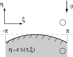
Figure 1: Curved interface as an $O(\epsilon)$-perturbation.

In the analysis of the RT instability we adopt the Kelvin’s restrictive assumption Drazin and Reid (2004), i.e. consider an inviscid and incompressible approximation of irrotational fluids. Let us transform from the laboratory system $(x,y,t)$ to the one moving with the interface with velocity $V(t)$ in the positive $y$-direction: $\left(\xi=x,\eta=y-\int_{0}^{t}{V(\widetilde{t})\,\mathrm{d}\widetilde{t}},\tau=t\right)$ and $(u,v)\rightarrow\left(\widetilde{u}=u,\widetilde{v}=v-V(t)\right)$, where tildas stand for the variables in the moving frame of reference. Then the potential function $\phi$, $\nabla\phi=(u,v)$, transforms into $\widetilde{\phi}=\phi-V(t)\,\eta$, where we put the arbitrary time-dependent constant of integration to zero without loss of generality. Since $V(t)$ is not constant, in general, then this new coordinate system is non-inertial and the full nonlinear system for the bulk (the harmonic equation for the potential $\widetilde{\phi}$ and the Lagrange-Cauchy integral for the pressure $p$) and interfacial dynamics (the normal stress and kinematic conditions) becomes

$$\left\{\begin{array}[]{c}\Delta\widetilde{\phi}=0,\\ \nabla\widetilde{\phi}\rightarrow 0,\ \eta\rightarrow-\infty,\end{array}\right.,\ \eta\leq\widetilde{f}$$ (2c)

$${\partial\widetilde{\phi}\over\partial\tau}+{|\nabla\widetilde{\phi}|^{2}\over 2}=-{p\over\rho}-\left(g+{\mathrm{d}V\over\mathrm{d}\tau}\right)\eta+C(\tau),\ \eta\leq\widetilde{f}$$ (2d)

$$p=-{\sigma\widetilde{f}_{\xi\xi}\over(1+\widetilde{f}_{\xi}^{2})^{3/2}},\ \eta=\widetilde{f}$$ (2e)

$${\partial\widetilde{f}\over\partial\tau}+{\partial\widetilde{\phi}\over\partial\xi}{\partial\widetilde{f}\over\partial\xi}={\partial\widetilde{\phi}\over\partial\eta},\ \eta=\widetilde{f},$$ (2f)

where $\nabla=\mathbf{i}\,\partial_{\xi}+\mathbf{j}\,\partial_{\eta}$, $\widetilde{f}(\tau,\xi)=f(t,x)-\int_{0}^{t}{V(\widetilde{t})\,\mathrm{d}\widetilde{t}}$ is the position of the interface in new coordinates. System (2) is the starting point of the stability analysis of curved interfaces; the key idea is to consider the curved interface locally, as depicted in figure 1, with small deviation from flatness, i.e. $\widetilde{f}(\tau,\xi)=\epsilon h(\tau,\xi)$ with $\epsilon\ll 1$.

As one can infer from system (2), there exists a base state solution, which is motionless, $\widetilde{\phi}^{0}=0$, and steady, $\widetilde{f}^{0}(\xi)$, if the conditions of static equilibrium are met, i.e.

$${\sigma\over\rho}{\widetilde{f}_{\xi\xi}\over(1+\widetilde{f}_{\xi}^{2})^{3/2}}-\left(g+{\mathrm{d}V\over\mathrm{d}\tau}\right)\widetilde{f}+C=0,$$ (3)

where constant $C$ is time-independent. Obviously, surface tension is required for the interface to have a non-zero curvature, while the pure RT case ${\mathrm{d}V/\mathrm{d}\tau}=a=\mathrm{const}$ allows the corresponding balance of the capillary and hydrostatic pressures.

Next, it is important to construct a general solution of the Laplace equation with non-fixed boundary values:

$$\begin{array}[]{c}\Delta\widetilde{\phi}=0,\\ \eta=\epsilon h(\xi):\ \widetilde{\phi}=\widetilde{\phi}_{0}(\xi),\end{array}$$ (6)

where $\widetilde{\phi}_{0}(\xi)$ is an arbitrary summable function to be determined from the free-boundary conditions. Here we restrict the consideration to even functions $h(x)$ and to the region in the neighborhood of the interface with the largest curvature, as sketched in figure 1. Without loss of generality, let the width of the domain be $2\pi$ (in non-dimensional coordinates: cf. figure 1). Then we can construct the most general velocity potential, which satisfies the Laplace equation in this region and allows one to solve the free-boundary problem. This constitutes the essence of the local approach. Since we are interested in a small, $O(\epsilon)$, perturbation of the boundary (cf. figure 1), then it is natural to appeal to the boundary perturbation method. Its basic idea Dyke (1975) is to transform the boundary conditions on the perturbed boundaries to that on the unperturbed boundaries, which are known.

The main outcome of this analysis is that despite the fact that the boundary is curved, as in figure 1, finite Fourier modes, $e^{inx}$, constitute a complete set of functions and thus allow one to build the solution to (6), which can be represented in the general form

$$\widetilde{\phi}(\tau,\xi,\eta)=\sum_{n\in\mathbb{N}}{A_{n}(\tau)e^{|n|\eta}e^{in\xi}}.$$ (7)

In this context, it is natural to comment on the ad hoc idea of Layzer Layzer (1955), which provided a break-through in the nonlinear modelling of the RT and RM instabilities. Layzer suggested approximating the potential function by $\widetilde{\phi}(\tau,\xi,\eta)=A(\tau)e^{\eta}\cos{\xi}$ near the tip of the bubble, which, apparently, is just one harmonic with $n=1$ out of the general expression (7) and which allowed him to derive a nonlinear evolution equation for the bubble amplitude $A(\tau)$. Using more terms from (7) one can get a more precise nonlinear model.

The equations for perturbations $\widetilde{f}^{\prime}$ and $\widetilde{\phi}^{\prime}$ linearized around the base state curved non-perturbed interface $\widetilde{f}^{0}(\xi)$ and $\widetilde{\phi}_{0}$ in the frame moving with the interface are given by:

$${\partial\widetilde{\phi}^{\prime}\over\partial\tau} =-\left(g+{\mathrm{d}V\over\mathrm{d}\tau}\right)\widetilde{f}^{\prime}+{\sigma\over\rho}\widetilde{f}^{\prime}_{\xi\xi}+o(\epsilon),$$ (8a)

$${\partial\widetilde{f}^{\prime}\over\partial\tau} =-\epsilon{\partial h^{0}\over\partial\xi}{\partial\widetilde{\phi}^{\prime}\over\partial\xi}+{\partial\widetilde{\phi}^{\prime}\over\partial\eta},$$ (8b)

at $\eta=\epsilon h^{0}(\xi)$. Here we used the fact that $\widetilde{f}^{0}(\xi)=\epsilon h^{0}(\xi)$, kept the terms up to $O(\epsilon)$ and excluded pressure. As we will see, the term of $O(\epsilon)$ will introduce a non-trivial correction to the stability results for flat interfaces.

Since ${\mathrm{d}V/\mathrm{d}\tau}=a=\mathrm{const}$, then system (8) contains no explicit time-dependence and therefore one can perform the standard eigenvalue analysis $\left[\widetilde{\phi}^{\prime}(\tau,\xi),\widetilde{f}^{\prime}(\tau,\xi)\right]\rightarrow\left[\Phi(\xi),F(\xi)\right]\,e^{\lambda\tau}$. The subsequent analysis is based on the well-established operator perturbation theory Kato (1966), which allows one to treat this problem as a regular (non-singular) perturbation problem:

$$\Phi(\xi)=\Phi^{0}+\epsilon\Phi^{1}+o(\epsilon),\ \lambda=\lambda_{0}+\epsilon\lambda_{1}+o(\epsilon),$$ (9)

which yields

$$\epsilon^{0} : \lambda_{0}^{2}\Phi^{0}+(g+a)\Phi^{0}_{\eta}-{\sigma\over\rho}\Phi^{0}_{\xi\xi\eta} =0,$$ (10a)

$$\epsilon^{1} : \lambda_{0}^{2}\Phi^{1}+(g+a)\Phi^{1}_{\eta}-{\sigma\over\rho}\Phi^{1}_{\xi\xi\eta} =-2\lambda_{0}\lambda_{1}\Phi^{0}$$ (10b)

$$+(g+a)h^{0}_{\xi}\Phi^{0}_{\xi}-{\sigma\over\rho}\left[h^{0}_{\xi\xi\xi}\Phi^{0}_{\xi}\right. \left.+2h^{0}_{\xi\xi}\Phi^{0}_{\xi\xi}+h^{0}_{\xi}\Phi^{0}_{\xi\xi\xi}\right].$$

Based on (7), potentials are given by

$$\Phi^{i}(\xi,\eta)=\sum_{n\in\mathbb{N}}{A_{n}^{i}e^{|n|\eta}e^{in\xi}}.$$ (11)

Substituting the zero-order approximation $\Phi^{0}(\xi,\eta)$ in (10a), evaluating at $\eta=0$, and projecting onto $e^{in\xi}$ yields

$$\lambda_{\pm 0}^{2}=-(g+a)|n|-(\sigma/\rho)|n|^{3}=0.$$ (12)

Next, substitution of $\Phi^{1}(\xi,\eta)$ into (10b) and projection onto $e^{in\xi}$ leads to vanishing of the left-hand side of (10b) in view of the definition of the zero-order eigenvalue (12), while the rest of (10b) results in

$$4\pi\lambda_{0}\lambda_{1}A_{m}^{1}=\sum_{n}{A_{n}^{1}}\int_{-\pi}^{\pi}\left\{in(g+a)h^{0}_{\xi}\right.$$

$$\left.-(\sigma/\rho)\left[i\,n\,h^{0}_{\xi\xi\xi}-2n^{2}h^{0}_{\xi\xi}-i\,n^{3}h^{0}_{\xi}\right]\right\}e^{i(n-m)\xi}\mathrm{d}\xi.$$

Since $\widetilde{\phi}^{\prime}(\tau,\xi)$ is real, and thus $\Phi^{i}(\xi,\eta)$ is real as well, then $A_{-r}=A_{r}$ and thus expansions (11) contain only cosines. Since $h^{0}(\xi)$ and $h^{0}_{\xi\xi}(\xi)$ are even functions of $\xi$, while $h^{0}_{\xi}(\xi)$ and $h^{0}_{\xi\xi\xi}(\xi)$ are odd, then integrals involving $h^{0}_{\xi}(\xi)$ and $h^{0}_{\xi\xi\xi}(\xi)$ should vanish. The only terms left are

$$4\pi\lambda_{0}\lambda_{1}A_{m}^{1}=-2{\sigma\over\rho}\sum_{n}{A_{n}^{1}\int_{-\pi}^{\pi}{n^{2}h^{0}_{\xi\xi}e^{i(n-m)\xi}\mathrm{d}\xi}}.$$

Since we perform the local analysis, then $h^{0}_{\xi\xi}\simeq\kappa=\mathrm{const}$ is the scaled $O(1)$ curvature and the first approximation for the eigenvalue becomes

$$\lambda_{\pm 1}^{(n)}\simeq{\sigma\over\rho}{n^{2}\over\lambda_{\pm 0}^{(n)}}\int_{-\pi}^{\pi}{h^{0}_{\xi\xi}\mathrm{d}\xi}.$$ (13)

Note that if the interface is non-symmetric, i.e. the odd derivatives $h^{0}_{\xi}(\xi)$ and $h^{0}_{\xi\xi\xi}(\xi)$ do not vanish, then these will affect the eigenvalue corrections; here we consider the symmetric case, as the leading order effect. Hence, we have proved the following

Assertion 1

If the flat interface is unstable in the RT case, i.e. there exists real $\lambda_{+0}^{(n)}>0$, then the addition of a positive curvature (concave interface: cf figure 2(a)) makes the physical system more unstable, while the addition of negative curvature (convex interface: cf figure 2(b)) makes the system less unstable. The eigenvalues obey

$$\lambda_{\pm}^{(n)}=\lambda_{\pm 0}^{(n)}+\epsilon\lambda_{\pm 1}^{(n)}+o(\epsilon),$$ (14)

with $\lambda_{\pm 0}^{(n)}$ and $\lambda_{\pm 1}^{(n)}$ given by (12) and (13), respectively.

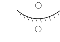
(a) Concave interface: $\kappa>0$.

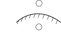
(b) Convex interface: $\kappa<0$.

Figure 2: Two generic curved interfaces; phase $1$ is the (heaviest) liquid phase.

In order to appreciate these results, let us make the following two corollary type clarifications. First, the interpretation of these curvature effects is not as trivial as one might expect, i.e. that the presence of surface tension tends to flatten the interface, since the curved interface base state is truly an equilibrium base state. Second, because of the curvature effect, the RT instability can be reversed, i.e. the sign of the growth rate can change as a function of base state curvature! Indeed, if the heavy phase $1$ accelerates the light phase $2$ and the interface is flat, then there should be no instability according to the RT criterion; however, if the interface is concave (cf. figure 2(a)), then the instability may appear. In fact, this can be illustrated with the well-known phenomena of vapor-filled underwater collapsing bubbles Birkhoff (1954); Plesset (1954), which are unstable despite that the denser liquid is accelerated towards the lighter vapor. Moreover, as indicated above, this instability result is unaffected by surface tension, which just allows for the existence of a base state (spherical bubble, in this case). The latter problem has been studied exactly because of its spherical symmetry, but to the author’s knowledge the conclusion that this is a particular case of the more general effect of interfacial curvature has never been established.

Lastly, it is known that the RT theory is valid only in the small amplitude limit, but when the interfacial distortions become significant the rate of their growth deviates significantly from predicted one by the RT theory Lewis (1950). Apparently, one of the sources of these deviations is due to finger formation and thus non-zero curvature: the fingers can be considered, in a quasi-static approximation, as a new base state which is subject to perturbations. The latter will have growth rate different from the case of a flat interface base state, as we just proved.

With the above understanding of the stability of two-dimensional (2D) weakly curved interfaces, one can easily address the stability of three-dimensional (3D) rims. Naturally, the main question of interest is the rim instability along $x$-axis, as shown schematically in figure 3. The idea is to analyze the structure of the solution near the rim tip. Then, the translation of the previous results onto the 3D case turns out to be straightforward, as suggested by the structure of the velocity potential solution, i.e. the solution of the 3D version of the problem (6). The zero- and first-order approximations read

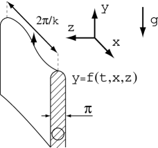
Figure 3: Three-dimensional rim.

$$\phi^{(j)}(x,y,z)=\sum_{n\in\mathbb{N}}{A_{n}^{(j)}e^{ikx}e^{\sqrt{k^{2}+|n|^{2}}y}e^{inz}},$$ (15)

with $j=1,2$ and therefore one gets the eigenvalue approximations $\lambda_{\pm 0}^{(n)}$ and $\lambda_{\pm 1}^{(n)}$ analogous to (12) and (13):

$$\lambda_{\pm 0}^{(n)} =\pm\left[-(g+a)\sqrt{k^{2}+|n|^{2}}-{\sigma\over\rho}\left(k^{2}+|n|^{2}\right)^{3/2}\right]^{1/2},$$

$$\lambda_{\pm 1}^{(n)} \simeq{\sigma\over\rho}{n^{2}\over\lambda_{\pm 0}^{(n)}}\int_{-\pi}^{\pi}{h^{0}_{\xi\xi}\mathrm{d}\xi},$$

i.e. the only difference is that the discrete wavenumber, $n$, (in $z$-direction) in (12) is replaced with the wavenumber in the $(x,z)$-plane, $\sqrt{k^{2}+|n|^{2}}$. This fact and equation (15) for the perturbation velocity field allow one to clearly see the previously made energy argument: the curvature affects the depth of penetration of a disturbance into the bulk and thus the factor $|k|$ in (1) is modified. In fact, for the long-wave perturbations of a rim of a liquid sheet of thickness $2\pi$, i.e. when $|k|\gg(2\pi)^{-1}$, the depth of penetration is $\sim 2\pi$ and therefore the factor $|k|$ in (1) is replaced by $(2\pi)^{-1}$. The latter of course changes the growth rate and the wavenumber selection. Since, the eigenvalue has the following structure:

$$\lambda=\lambda_{0}(k;n)+C(n)\kappa,$$ (16)

where $\kappa$ is the curvature, then the curvature in $z$-direction has an effect on the wavenumber selection in $x$-direction, as one can learn from figure 4. Namely, concave interfaces enlarge the range of unstable wavelength for fixed surface tension (dashed line in figure 4), while convex interfaces, as in figure 3, stabilize the physical system and thus narrow the range of unstable wavenumbers (dotted line in figure 4). Thus, the analysis of 3D curved interfaces can be summarized as follows

Assertion 2

The stability of 3D rims, as that shown in figure 3, is affected by the transverse curvature: concave interfaces are less stable than flat ones, while convex interfaces are more stable. The range of lengthwise-unstable wavenumbers (i.e. along-the-rim wavenumbers) is narrowed in the case of convex interfaces and widened in the case of concave interfaces.

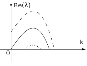
Figure 4: Effect of the interfacial curvature on the eigenvalues in the 3D case. Solid curve corresponds to zero curvature, dashed line to concave interface (positive curvature), and dotted line to convex interface (negative curvature).

In conclusion, the main contribution of this study is the clarification of the interfacial curvature effects in the 2D and 3D cases on the growth rate and the wavenumber selection of the Rayleigh-Taylor instability. All the major results are summarized in Assertions 1-2, and can be easily extended onto the case of Richtmyer-Meshkov instability. The analysis of the stability of curved interfaces also leads to the rigorous generalization of the classical idea due to Layzer (1955) on approximating the potential function in free-boundary problems with curved base state interfaces. While the base state interfacial curvature considered in this Letter is due to the presence of surface tension (for the sake of mathematical concreteness), it should have analogous implications for the stability characteristics regardless of its physical origins.