The problem of the body of revolution of minimal resistance

Abstract

Newton’s problem of the body of minimal aerodynamic resistance is traditionally stated in the class of convex axially symmetric bodies with fixed length and width. We state and solve the minimal resistance problem in the wider class of axially symmetric but generally nonconvex bodies. The infimum in this problem is not attained. We construct a sequence of bodies minimizing the resistance. This sequence approximates a convex body with smooth front surface, while the surface of approximating bodies becomes more and more complicated. The shape of the resulting convex body and the value of minimal resistance are compared with the corresponding results for Newton’s problem and for the problem in the intermediate class of axisymmetric bodies satisfying the single impact assumption [8]. In particular, the minimal resistance in our class is smaller than in Newton’s problem; the ratio goes to $1/2$ as (length)/(width of the body) $\to 0$, and to $1/4$ as (length)/(width) $\to+\infty$.

Mathematics subject classifications: 49K30, 49Q10

Key words and phrases: Newton’s problem, bodies of minimal resistance, calculus of variations, billiards

Running title: Problem of minimal resistance

1 Introduction

In 1687, I. Newton in his Principia [1] considered a problem of minimal resistance for a body moving in a homogeneous rarefied medium. In slightly modified terms, the problem can be expressed as follows.

A convex body is placed in a parallel flow of point particles. The density of the flow is constant, and velocities of all particles are identical. Each particle incident on the body makes an elastic reflection from its boundary and then moves freely again. The flow is very rare, so that the particles do not interact with each other. Each incident particle transmits some momentum to the body; thus, there is created a force of pressure on the body; it is called aerodynamic resistance force, or just resistance.

Newton described (without proof) the body of minimal resistance in the class of convex and axially symmetric bodies of fixed length and maximal width, where the symmetry axis is parallel to the flow velocity. That is, any body from the class is inscribed in a right circular cylinder with fixed height and radius. The rigorous proof of the fact that the body described by Newton is indeed the minimizer was given two centuries later. From now on, we suppose that the radius of the cylinder equals 1 and the height equals $h$, with $h$ being a fixed positive number. The cylinder axis is vertical, and the flow falls vertically downwards. The body of least resistance for $h=2$ is shown on fig. 1.

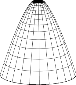
Figure 1: The Newton solution for $h=2$.

Since the early 1990s, there have been obtained new interesting results related to the problem of minimal resistance in various classes of admissible bodies [2]-[12]. In particular, there has been considered the wider class of convex (generally non-symmetric) bodies inscribed in a given cylinder [2]-[4],[7],[10]. It was shown that the solution in this class exists and does not coincide with the Newton one. The problem is not completely solved till now. The numerical solution for $h=1.5$ is shown on fig. 2.

Figure 2: The non-symmetric solution for $h=1.5$.

By removing both assumptions of symmetry and convexity, one gets the (even wider) class of bodies inscribed in a given cylinder. More precisely, a generic body from the class is a connected set with piecewise smooth boundary which is contained in the cylinder, contains an orthogonal cross section of the cylinder, and satisfies a regularity condition to be specified below. Notice that there may occur multiple reflections of particles from the surface of a non-convex body, while reflections from convex bodies are always single. The problem of minimal resistance in this class was solved in [11, 12]. In contrast to the class of convex $\&$ axisymmetric bodies and the class of convex bodies, the infimum of resistance here equals zero, and we believe the infimum cannot be attained.

In addition to the classes of admissible bodies discussed above:
      (i) convex $\&$ axisymmetric (the classical Newton problem);
      (ii) convex but generally non-symmetric;
      (iii) generally nonconvex and non-symmetric,
there remains a class that has not been studied as yet:
      (iv) axisymmetric but generally nonconvex bodies.
The aim of this paper is to fill this gap: we shall solve the minimal resistance problem for the fourth class.

Note that in the paper [8] there was considered the intermediate class of
      (v) axially symmetric nonconvex bodies, under the additional so-called
           "single impact assumption".
This geometric assumption on the body’s shape means that each particle hits the body at most once; multiple reflections are not allowed. On the contrary, multiple reflections are allowed in our setting; we only assume that the body’s boundary is piecewise smooth and satisfies the regularity condition stated below.

The class (v) is intermediate between the classes (i) and (iv); it contains the former one and is contained in the latter one. We shall determine the minimal resistance and the minimizing sequence of bodies for the class (iv) (which will be referred to as nonconvex case), and compare them with the corresponding results for the class (i) (Newton case) and for the class (v) (single impact case).

Consider a compact connected set $B\subset{\mathbb{R}}^{3}$ and choose an orthogonal reference system $Oxyz$ in such a way that the axis $Oz$ is parallel to the flow direction; that is, the particles move vertically downwards with the velocity $(0,0,-1)$. Suppose that a flow particle (or, equivalently, a billiard particle in ${\mathbb{R}}^{3}\setminus B$) with coordinates $x(t)=x$,  $y(t)=y$,  $z(t)=-t$ makes a finite number of reflections at regular points of the boundary $\partial B$ and moves freely afterwards. Denote by $\nu_{B}(x,y)$ the final velocity. If there are no reflections, put $\nu_{B}(x,y)=(0,0,-1)$.

Thus, one gets the function $\nu_{B}=(\nu_{B}^{x},\nu_{B}^{y},\nu_{B}^{z})$ taking values in $S^{2}$ and defined on a subset of ${\mathbb{R}}^{2}$. We impose the regularity condition requiring that $\nu_{B}$ is defined on a full measure subset of ${\mathbb{R}}^{2}$. All convex sets $B$ satisfy this condition; examples of non-convex sets violating it are given on figure 3. Both sets are of the form $B=G\times[0,\,1]\subset{\mathbb{R}}^{2}_{x,z}\times R^{1}_{y}$, with $G$ being shown on the figure. On fig. 3a, a part of the boundary is an arc of parabola with the focus $F$ and with the vertical axis. Incident particles, after making a reflection from the arc, get into the singular point $F$ of the boundary. On fig. 3b, one part of the boundary belongs to an ellipse with foci $F_{1}$ and $F_{2}$, and another part, $AB$, belongs to a parabola with the focus $F_{1}$ and with the vertical axis. After reflecting from $AB$, particles of the flow get trapped in the ellipse, making infinite number of reflections and approaching the line $F_{1}F_{2}$ as time goes to $+\infty$. In both cases, $\nu_{\cal B}$ is not defined on the corresponding positive-measure subsets of ${\mathbb{R}}^{2}$.

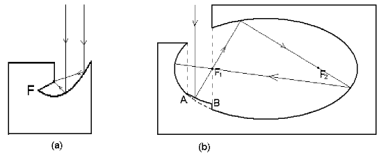
Figure 3: (a) After reflecting from the arc of parabola, the particles get into the singular point $F$. (b) After reflecting from the arc of parabola $AB$, the particles get trapped in the ellipse.

Each particle interacting with the body $B$ transmits to it the momentum equal to the particle mass times $\left((0,0,-1)-\nu_{B}(x,y)\right)$. Summing up over all momenta transmitted per unit time, one obtains that the resistance of $B$ equals $-\rho\,\mathrm{R}(B)$, where

$$\mathrm{R}(B)=\int\!\!\!\!\int_{{\mathbb{R}}^{2}}\left(\nu_{B}^{x},\,\nu_{B}^{y},\,1+\nu_{B}^{z}\right)dx\,dy,$$

and $\rho$ is the flow density. One is usually interested in minimizing the third component of $\mathrm{R}(B)$,

$$\mathrm{R}_{z}(B)=\int\!\!\!\!\int_{{\mathbb{R}}^{2}}\left(1+\nu_{B}^{z}(x,y)\right)dx\,dy.$$ (1)

If $B$ is convex then the upper part of the boundary $\partial B$ is the graph of a concave function $w(x,y)$. Besides, there is at most one reflection from the boundary, and the velocity of the reflected particle equals $\nu_{B}(x,y)=(1+|\nabla w|^{2})^{-1}(-2w_{x},\,-2w_{y},\,1-|\nabla w|^{2})$. Therefore, the formula (1) takes the form

$$\mathrm{R}_{z}(B)=\int\!\!\!\!\int\frac{2}{1+|\nabla w(x,y)|^{2}}\ dx\,dy,$$ (2)

the integral being taken over the domain of $w$.

Further, if $B$ is a convex axially symmetric body then (in a suitable reference system) the function $w$ is radial: $w(x,y)=f(\sqrt{x^{2}+y^{2}})$, therefore one has

$$\mathrm{R}_{z}(B)=2\pi\!\int\!\frac{2r}{1+f^{\prime 2}(r)}\ dr,$$ (3)

the integral being taken over the domain of $f$.

Thus, in the cases (i), (ii), and (v) the problem of minimal resistance reads as follows:

$$\text{(i) \, \ \ \ \ \ \ \ minimize}\ \ \ \ \int_{0}^{1}\frac{r}{1+f^{\prime 2}(r)}\ dr\hskip 156.49014pt$$ (4)

over all concave monotone non-increasing functions $f:[0,\,1]\to[0,\,h]$;

$$\text{(ii) \ \ \ minimize}\ \ \int\!\!\!\!\int_{\Omega}\,\frac{1}{1+|\nabla w(x,y)|^{2}}\ dx\,dy\hskip 142.26378pt$$

over all concave functions $w:\Omega\to[0,\,h]$, where $\Omega=\{x^{2}+y^{2}\leq 1\}$ is the

unit circle;

(v) minimize the functional (4) over the set $$\mathcal{C}_{h} f:[0,\,1]\to[0,\,h]$$ of functions

satisfying the single impact condition (see [8], formulas (3) and (1)).

In the nonconvex cases (iii) and (iv) the functional to be minimized (1) cannot be written down explicitly in terms of the body’s shape. Still, in the radial case (iv) it can be simplified in the following way.

Let $B$ be a compact connected set inscribed in the cylinder $x^{2}+y^{2}\leq 1$,  $0\leq z\leq h$ and possessing rotational symmetry with respect to the axis $Oz$. This set is uniquely defined by its vertical central cross section $G=\{(x,z):(x,0,z)\in B\}$. It is convenient to reformulate the problem in terms of the set $G$.

Consider the billiard in ${\mathbb{R}}^{2}\setminus G$ and suppose that a billiard particle initially moves according to $x(t)=x$,  $z(t)=-t$, then makes a finite number of reflections (maybe none) at regular points of $\partial G$, and finally moves freely with the velocity $v_{G}(x)=(v_{G}^{x}(x),v_{G}^{z}(x))$. The regularity condition now means that that the so determined function $v_{G}$ is defined for almost every $x$. One can see that $\nu_{B}^{x}(x,y)=(x/\!\sqrt{x^{2}+y^{2}})v_{G}^{x}(\sqrt{x^{2}+y^{2}})$,  $\nu_{B}^{y}(x,y)=(y/\!\sqrt{x^{2}+y^{2}})v_{G}^{y}(\sqrt{x^{2}+y^{2}})$, and $\nu_{B}^{z}(x,y)=v_{G}^{z}(\sqrt{x^{2}+y^{2}})$. It follows that $\mathrm{R}_{x}(B)=0=\mathrm{R}_{y}(B)$ and $\mathrm{R}_{z}(B)=2\pi\int_{0}^{1}(1+v_{G}^{z}(x))\,x\,dx$. Thus, our minimization problem takes the form

$$\inf_{G\in{\cal G}_{h}}R(G),\ \ \ \text{where}\ \ R(G)=\int_{0}^{1}\!\left(1+v_{G}^{z}(x)\right)x\,dx$$ (5)

and ${\cal G}_{h}$ is the class of compact connected sets $G\subset{\mathbb{R}}^{2}$ with piecewise smooth boundary that are inscribed in the rectangle $-1\leq x\leq 1$,  $0\leq z\leq h$, are symmetric with respect to the axis $Oz$, and satisfy the regularity condition (see fig. 4).

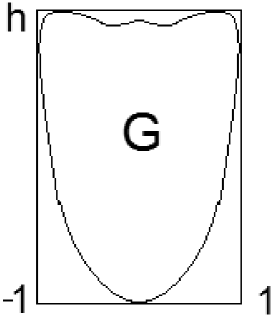
Figure 4: A set $G\in{\cal G}_{h}$.

The main results are stated in section 2: the minimization problem is solved and the solution is compared with the Newton solution (case (i)) and the single-impact solution (case (v)). Details of all proofs are put in section 3.

2 Statement of the results

Denote by ${\cal G}_{h}^{\text{c}onv}$ the class of convex sets from ${\cal G}_{h}$. One can easily see that if $G\in{\cal G}_{h}$ then conv$\,G\in{\cal G}_{h}^{\text{c}onv}$. For $G\subset{\cal G}_{h}^{\text{c}onv}$ define the modified law of reflection as follows. A particle initially moves vertically downwards according to $x(t)=x$,  $z(t)=-t$ and reflects at a regular point of the boundary $\partial G$; at this point the velocity instantaneously changes to $\hat{v}_{G}(x)=(\hat{v}_{G}^{x}(x),\hat{v}_{G}^{z}(x))$, where $\hat{v}_{G}(x)$ is the unit vector tangent to $\partial G$ such that $\hat{v}_{G}^{z}(x)\leq 0$ and $x\cdot\hat{v}_{G}^{x}(x)\geq 0$ (see fig. 5).

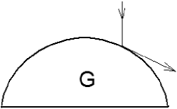
Figure 5: Modified reflection law.

The set $G\in{\cal G}_{h}$ is bounded above by the graph of a concave even function $z=f_{G}(x)$. For $x>0$, one has

$$\hat{v}_{G}(x)=\frac{(1,f^{\prime}_{G}(x))}{\sqrt{1+f^{\prime 2}_{G}(x)}}\,.$$ (6)

The resistance of $G$ under the modified reflection law equals $(0,-\widehat{R}(G))$, where

$$\widehat{R}(G)=\int_{0}^{1}(1+\hat{v}^{z}_{G}(x))\,x\,dx\,.$$ (7)

Taking into account (6), one gets

$$\widehat{R}(G)=\int_{0}^{1}\left(1+\frac{f^{\prime}_{G}(x)}{\sqrt{1+f^{\prime 2}_{G}(x)}}\right)x\,dx;$$ (8)

the function $f_{G}$ is concave, nonnegative, and monotone non-increasing, with $f(0)=h$.

Theorem 1.

$$\inf_{G\in{\cal G}_{h}}R(G)=\inf_{G\in{\cal G}_{h}^{\text{c}onv}}\widehat{R}(G).$$ (9)

This theorem follows from the following lemmas 1 and 2 which will be proved in the next section.

Lemma 1.

For any $G\in\mathcal{G}_{h}$ one has

$$R(G)\geq\widehat{R}(\text{conv}\,G).$$

Lemma 2.

Let $G\in{\cal G}_{h}^{\text{c}onv}$. Then there exists a sequence of sets $G_{n}\in{\cal G}_{h}$ such that

$$\lim_{n\to\infty}R(G_{n})=\widehat{R}(G).$$

Indeed, lemma 1 implies that $\inf_{G\in{\cal G}_{h}}R(G)\geq\inf_{G\in{\cal G}_{h}^{\text{c}onv}}\widehat{R}(G)$, and lemma 2 implies that $\inf_{G\in{\cal G}_{h}}R(G)\leq\inf_{G\in{\cal G}_{h}^{\text{c}onv}}\widehat{R}(G)$.

Theorem 1 allows one to state the minimization problem (5) in an explicit form. Namely, taking into account (8) and putting $f=h-f_{G}$, one rewrites the right hand side of (9) as

$$\inf_{f\in{\cal F}_{h}}\int_{0}^{1}\left(1-\frac{f^{\prime}(x)}{\sqrt{1+f^{\prime 2}(x)}}\right)x\,dx,$$ (10)

where ${\cal F}_{h}$ is the set of convex monotone non-decreasing functions $f:[0,\,1]\to[0,\,h]$ such that $f(0)=0$. The solution of (10) is provided by the following general theorem.

Consider a positive piecewise continuous function $p$ defined on ${\mathbb{R}}_{+}:=[0,\,+\infty)$ and converging to zero as $u\to+\infty$, and consider the problem

$$\inf_{f\in{\cal F}_{h}}\mathcal{R}[f],\leavevmode\nobreak\ \leavevmode\nobreak\ \leavevmode\nobreak\ \text{where}\leavevmode\nobreak\ \leavevmode\nobreak\ \leavevmode\nobreak\ \mathcal{R}[f]=\int_{0}^{1}p(f^{\prime}(x))\,x\,dx.$$ (11)

Denote by $\bar{p}(u)$,  $u\in{\mathbb{R}}_{+}$ the greatest convex function that does not exceed $p(u)$. Put $\xi_{0}=-1/\bar{p}^{\prime}(0)$ and $u_{0}=\inf\{u>0:\,\bar{p}(u)=p(u)\}$. One always has $\xi_{0}\geq 0$; if $u_{0}=0$ and there exists $p^{\prime}(0)$ then $\xi_{0}=-1/p^{\prime}(0)$, and if $u_{0}>0$ then $\xi_{0}=u_{0}/(p(0)-p(u_{0}))$. Denote by $u=\upsilon(z)$,  $z\geq\xi_{0}$ the generalized inverse of the function $z=-1/\bar{p}^{\prime}(u)$, that is, $\upsilon(z)=\sup\{u:-1/\bar{p}^{\prime}(u)\leq z\}$. By $\Upsilon$, denote the primitive of $\upsilon$:  $\Upsilon(z)=\int_{\xi_{0}}^{z}\upsilon(\xi)d\xi$,  $z\geq\xi_{0}$. Finally, put $\mathcal{R}(h):=\inf_{f\in{\cal F}_{h}}\mathcal{R}[f]$.

Theorem 2.

For any $h>0$ the solution $f_{h}$ of the problem (11) exists and is uniquely determined by

$$f_{h}(x)=\left\{\begin{array}[]{ll}0&\text{if}\leavevmode\nobreak\ \leavevmode\nobreak\ 0\leq x\leq x_{0}\\ \frac{1}{z}\,\Upsilon(zx)&\text{if}\leavevmode\nobreak\ \leavevmode\nobreak\ x_{0}<x\leq 1\,,\end{array}\right.$$ (12)

where $z=z(h)$ is a unique solution of the equation

$$\Upsilon(z)=zh$$ (13)

and $x_{0}=x_{0}(h)=\xi_{0}/z(h)$. Further, one has $f_{h}^{\prime}(x_{0}+0)=u_{0}$. The function $x_{0}(h)$ is continuous and $x_{0}(0)=1$. The minimal resistance equals

$$\mathcal{R}(h)\ =\ \frac{1}{2}\left(\bar{p}(\upsilon(z))\,+\,\frac{\upsilon(z)-h}{z}\right);$$ (14)

in particular, $\mathcal{R}(0)=p(0)/2$.

If, additionally, the function $p$ satisfies the asymptotic relation $p(u)=cu^{-\alpha}\,(1+o(1))$ as $u\to+\infty$,  $c>0$,  $\alpha>0$ then

$$x_{0}(h)=c\alpha\left(\frac{\alpha+1}{\alpha+2}\right)^{\alpha+1}\xi_{0}h^{-\alpha-1}(1+o(1)),\leavevmode\nobreak\ \leavevmode\nobreak\ h\to+\infty,$$ (15)

and

$$\mathcal{R}(h)=\frac{c}{2}\left(\frac{\alpha+1}{\alpha+2}\right)^{\alpha+1}h^{-\alpha}(1+o(1)),\leavevmode\nobreak\ \leavevmode\nobreak\ h\to+\infty.$$ (16)

Let us apply the theorem to the three cases under consideration.

1. First consider the non-convex case. The problem (10) we are interested in is a particular case of (11) with $p(u)=p_{\text{n}c}(u):=1-u/\sqrt{1+u^{2}}$ (the subscript "nc" stands for "non-convex"). The function $p_{\text{n}c}$ itself, however, is convex, hence $u_{0}=0$ and $\bar{p}_{\text{n}c}\equiv p_{\text{n}c}$. Further, one has $-1/\bar{p}^{\prime}_{\text{n}c}(u)=(1+u^{2})^{3/2}$, therefore $\upsilon_{\text{n}c}(z)=\sqrt{z^{2/3}-1}$,  $\xi_{0}^{\text{n}c}=1$, and

$$\Upsilon_{\text{n}c}(z)=\frac{3}{8}(2z^{2/3}-1)z^{1/3}\sqrt{z^{2/3}-1}-\frac{3}{8}\ln(z^{1/3}+\sqrt{z^{2/3}-1}).$$ (17)

The formulas (17), (13), and (12) with $x_{0}=1/z$, determine the solution of (10). Notice that, as opposed to the Newton case, the solution is given by the explicit formulas. However, they contain the parameter $z$ to be defined implicitly from (13).

Further, according to theorem 2, $f^{\prime}_{h}(x_{0}+0)=0=f^{\prime}_{h}(x_{0}-0)$,  $x_{0}=x_{0}^{\text{n}c}$, hence the solution $f_{h}$ is differentiable everywhere in $(0,\,1)$. Besides, one has

$$x_{0}^{\text{n}c}(h)=\frac{27}{64}\,h^{-3}(1+o(1))\ \ \ \ \text{as}\ \ h\to+\infty.$$ (18)

The minimal resistance is calculated according to (14); after some algebra one gets

$$\mathcal{R}_{\text{n}c}(h)\,=\,\frac{1}{2}\,+\,\frac{3+2z^{2/3}-8z^{4/3}}{16z^{5/3}}\,\sqrt{z^{2/3}-1}\,+\,\frac{3}{16z^{2}}\,\ln(z^{1/3}+\sqrt{z^{2/3}-1}).$$

One also gets from theorem 2 that $\mathcal{R}_{\text{n}c}(0)=0.5$ and

$$\mathcal{R}_{\text{n}c}(h)=\frac{27}{128}h^{-2}(1+o(1))\ \ \ \ \text{as}\ \ h\to+\infty.$$ (19)

2. The original Newton problem (case (i) in our classification) is also a particular case of (11), with $p(u)=p_{N}(u):=2/(1+u^{2})$. One has $u_{0}=1$ and $\bar{p}_{N}(u)=\left\{\begin{array}[]{ll}\leavevmode\nobreak\ 2-u&\text{if }\,0\leq u\leq 1\\ 2/(1+u^{2})&\text{if }\leavevmode\nobreak\ \leavevmode\nobreak\ \leavevmode\nobreak\ u\geq 1\leavevmode\nobreak\ \leavevmode\nobreak\ ,\end{array}\right.$ and after some calculation one gets that $\xi^{N}_{0}=1$ and the function $\Upsilon_{N}(z)$,  $z\geq 1$, in a parametric representation, is $\Upsilon_{N}=\frac{1}{4}\,(3u^{4}/4+u^{2}-\ln u-7/4)$,  $z=(1+u^{2})^{2}/(4u)$,  $u\geq 1$. From here one obtains the well-known Newton solution:  if $0\leq x\leq x_{0}$ then $f_{h}(x)=0$, and if $x_{0}<x\leq 1$ then $f_{h}$ is defined parametrically: $f_{h}=\frac{x_{0}}{4}\,(3u^{4}/4+u^{2}-\ln u-7/4)$,  $x=\frac{x_{0}}{4}\,\frac{(1+u^{2})^{2}}{u}$, where $x_{0}=4u_{*}/(1+u_{*}^{2})^{2}$ and $u_{*}$ is determined from the equation $(3u_{*}^{4}/4+u_{*}^{2}-\ln u_{*}-7/4)\,u_{*}/(1+u_{*}^{2})^{2}=h$. The function $f_{h}$ is not differentiable at $x_{0}$: one has $f^{\prime}_{h}(x_{0}+0)=1$ and $f^{\prime}_{h}(x_{0}-0)=0$.

One also has $\mathcal{R}_{N}(0)=1$,

$$\mathcal{R}_{N}(h)=\frac{27}{32}h^{-2}(1+o(1))\ \ \ \ \text{as}\ \ h\to+\infty.$$ (20)

and

$$x_{0}^{N}(h)=\frac{27}{16}\,h^{-3}(1+o(1))\ \ \ \ \text{as}\ \ h\to+\infty.$$ (21)

3. The minimal problem in the single impact case with $h>M^{*}\approx 0.54$ can also be reduced to (11), with $p(u)=p_{\text{s}i}(u):=\left\{\begin{array}[]{ll}\leavevmode\nobreak\ p^{*}&\text{if }\,u=0\\ 2/(1+u^{2})&\text{if }\leavevmode\nobreak\ \leavevmode\nobreak\ \leavevmode\nobreak\ u>0\leavevmode\nobreak\ \leavevmode\nobreak\ ,\end{array}\right.$ where $p^{*}=8(\ln(8/5)+\arctan(1/2)-\pi/4)\approx 1.186$. This fact can be easily deduced from [8]; for the reader’s convenience we put the details of derivation in the next section. From the above formula one can calculate that $u_{0}\approx 1.808$ and $\xi_{0}^{\text{s}i}\approx 2.52$.

The asymptotic formulas here take the form

$$x_{0}^{\text{s}i}(h)=\xi_{0}^{\text{s}i}\cdot x_{0}^{N}(h)(1+o(1))\ \ \ \ \text{as}\ \ h\to+\infty$$ (22)

and

$$\mathcal{R}_{\text{s}i}(h)=\frac{27}{32}h^{-2}(1+o(1))\ \ \ \ \text{as}\ \ h\to+\infty.$$ (23)

Finally, using the results of [8], one can show that $\mathcal{R}_{\text{s}i}(0)=\pi/2-2\arctan(1/2)\approx 0.6435$. This will also be made in the next section.

Now we are in a position to compare the solutions in the three cases. One obviously has $\mathcal{R}_{\text{n}c}(h)\leq\mathcal{R}_{\text{s}i}(h)\leq\mathcal{R}_{N}(h)$. From the above formulas one sees that $\mathcal{R}_{\text{n}c}(0)=0.5$,  $\mathcal{R}_{N}(0)=1$, and $\mathcal{R}_{\text{s}i}(0)\approx 0.6435$. Besides, one has $\lim_{h\to+\infty}({\mathcal{R}_{\text{n}c}(h)}/{\mathcal{R}_{N}(h)})=1/4$ and $\lim_{h\to+\infty}({\mathcal{R}_{\text{s}i}(h)}/{\mathcal{R}_{N}(h)})=1$. Thus, for "short" bodies, the minimal resistance in the nonconvex case is two times smaller than in the Newton case, and $22\%$ smaller, as compared to the single impact case. For "tall" bodies, the minimal resistance in the nonconvex case is four times smaller as compared th the Newton case, while the minimal resistance in the Newton case and in the single impact case are (asymptotically) the same.

In the three cases of interest, the convex hull of the three-dimensional optimal body of revolution has a flat disk of radius $x_{0}(h)$ at the front part of its boundary. One always has $x_{0}(0)=1$. For "tall" bodies, one has $\lim_{h\to+\infty}(x_{0}^{\text{n}c}(h)/x_{0}^{N}(h))=1/4$ and $\lim_{h\to+\infty}(x_{0}^{\text{s}i}(h)/x_{0}^{N}(h))=\xi_{0}^{\text{s}i}\approx 2.52$; that is, the disk radius in the non-convex case and in the single impact case is, respectively, 4 times smaller and $2.52$ times larger, as compared to the Newton case.

Besides, in the nonconvex case, the front part of the surface of the body’s convex hull is smooth. On the contrary, in the Newton case, the front part of the body’s surface has singularity at the boundary of the front disk.

3 Proofs of the results

3.1 Proof of lemma 1

It suffices to show that

$$v^{z}_{G}(x)\geq\hat{v}^{z}_{\text{conv}\,G}(x)\ \ \text{for any}\ \ x\in[0,\,1].$$ (24)

Consider two scenarios of motion for a particle that initially moves vertically downwards, $x(t)=x$ and $z(t)=-t$. First, the particle hits conv $G$ at a point $r_{0}\in\partial(\text{conv}\,G)$ according to the modified reflection law and then moves with the velocity $\hat{v}_{\text{conv}\,G}(x)$. Second, it hits $G$ (possibly several times) according to the law of elastic reflection, and then moves with the velocity $v_{G}(x)$. Denote by $n$ the outer unit normal to $\partial(\text{conv}\,G)$ at $r_{0}$; on fig. 6 there are shown two possible cases: $\,r_{0}\in\partial G$ and $r_{0}\not\in\partial G$.

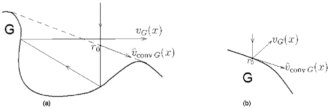
Figure 6: Two scenarios of reflection.

It is easy to see that

$$\langle v_{G}(x),n\rangle\geq 0,$$ (25)

where $\langle\cdot\,,\cdot\rangle$ means the scalar product. Indeed, denote by $r(t)=(x(t),z(t))$ the particle position at time $t$. At some instant $t_{1}$ the particle intersects $\partial(\text{conv}\,G)$ and then moves outside $\text{conv}\,G$. The function $\langle r(t),n\rangle$ is linear and satisfies $\langle r(t),n\rangle\geq\langle r(t_{1}),n\rangle$ for $t\geq t_{1}$, therefore its derivative $\langle v_{G}(x),n\rangle$ is positive.

>From (25) and the relations $\langle\hat{v}_{\text{conv}\,G}(x),n\rangle=0$,  $\hat{v}^{z}_{\text{conv}\,G}(x)\leq 0$ and $n_{z}\geq 0$,  $n_{x}\geq 0$ one gets (24).

3.2 Proof of lemma 2

Take a family of piecewise affine even functions $f_{\varepsilon}:[-1,\,1]\to[0,\,h]$ such that $f_{\varepsilon}^{\prime}$ uniformly converges to $f_{G}^{\prime}$ as $\varepsilon\to 0^{+}$. Require also that the functions $f_{\varepsilon}$ are concave and monotone decreasing as $x>0$, and $f_{\varepsilon}(0)=h$,  $f_{\varepsilon}(1)=f_{G}(1)$. Consider the family of convex sets $G_{\varepsilon}\in{\cal G}_{h}^{\text{c}onv}$ bounded from above by the graph of $f_{\varepsilon}$ and from below, by the segment $-1\leq x\leq 1$,  $z=0$. Taking into account (8), one gets $\lim_{\varepsilon\to 0^{+}}\widehat{R}(G_{\varepsilon})=\widehat{R}(G)$.

Below we shall determine a family of sets $G_{\varepsilon,\delta}\in{\cal G}_{h}$ such that $\lim_{\delta\to 0^{+}}R(G_{\varepsilon,\delta})=\widehat{R}(G_{\varepsilon})$ and next, using the diagonal method, select a sequence $\varepsilon_{n}\to 0,\ \delta_{n}\to 0$ such that $\lim_{n\to\infty}R(G_{\varepsilon_{n},\delta_{n}})=\lim_{n\to\infty}\widehat{R}(G_{\varepsilon_{n}})=\widehat{R}(G)$. This will finish the proof.

Fix $\varepsilon>0$ and denote by $-1=x_{-m}<x_{-m+1}<\ldots<x_{0}=0<\ldots<x_{m}=1$ the jump values of the piecewise constant function $f^{\prime}_{\varepsilon}$. (One obviously has $x_{-i}=-x_{i}$.) For each $i=1,\ldots,m$ we shall define a non self-intersecting curve $l^{i,\varepsilon,\delta}$ that connects the points $(x_{i-1},f_{\varepsilon}(x_{i-1}))$ and $(x_{i},f_{\varepsilon}(x_{i}))$ and is contained in the quadrangle $x_{i-1}\leq x\leq x_{i}$,  $f_{\varepsilon}(x_{i})\leq z\leq f_{\varepsilon}(x_{i-1})+(f^{\prime}_{\varepsilon}(x_{i-1}+0)+\delta)\cdot(x-x_{i-1})$. The curve $l^{-i,\varepsilon,\delta}$ is by definition symmetric to $l^{i,\varepsilon,\delta}$ with respect to the axis $Oz$. Let now $l^{\varepsilon,\delta}:=\cup_{-m\leq i\leq m}l^{i,\varepsilon,\delta}$ and let $G_{\varepsilon,\delta}$ be the set bounded by the curve $l^{\varepsilon,\delta}$, by the two vertical segments $0\leq z\leq f_{\varepsilon}(1)$,  $x=\pm 1$, and by the horizontal segment $-1\leq x\leq 1$,  $z=0$.

For an interval $I\subset[0,\,1]$, define

$$\widehat{R}_{I}(G_{\varepsilon}):=\int_{I}(1+\hat{v}_{G_{\varepsilon}}^{z}(x))\,x\,dx$$ (26)

and

$$R_{I}(G_{\varepsilon,\delta}):=\int_{I}(1+v_{G_{\varepsilon,\delta}}^{z}(x))\,x\,dx.$$ (27)

Denote $I_{i}=[x_{i-1},\,x_{i}]$; one obviously has $\widehat{R}(G_{\varepsilon})=\sum_{i=1}^{m}\widehat{R}_{I_{i}}(G_{\varepsilon})$ and $R(G_{\varepsilon,\delta})=\sum_{i=1}^{m}R_{I_{i}}(G_{\varepsilon,\delta})$. Thus, it remains to determine the curve $l^{i,\varepsilon,\delta}$ and prove that

$$\lim_{\delta\to 0^{+}}R_{I_{i}}(G_{\varepsilon,\delta})=\widehat{R}_{I_{i}}(G_{\varepsilon}).$$ (28)

This will complete the proof of the lemma.

Note that for $x\in I_{i}$,  $i=1,\ldots,m$ holds

$$\hat{v}^{z}_{G_{\varepsilon}}=\frac{f^{\prime}_{\varepsilon}(x_{i-1}+0)}{\sqrt{1+(f^{\prime}_{\varepsilon}(x_{i-1}+0))^{2}}}.$$ (29)

Fix $\varepsilon$ and $i$ and mark the points $P=(x_{i-1},f_{\varepsilon}(x_{i-1}))$,  $P^{\prime}=(x_{i},f_{\varepsilon}(x_{i}))$,  $Q=(x_{i-1},f_{\varepsilon}(x_{i}))$, and $S=(x_{i},\,f_{\varepsilon}(x_{i-1})+(f^{\prime}_{\varepsilon}(x_{i-1}+0)+\delta)\cdot(x_{i}-x_{i-1}))$; see fig. 7. Mark also the point $Q_{\delta}=(x_{i-1}+\delta,f_{\varepsilon}(x_{i}))$, which is located on the segment $QP^{\prime}$ at the distance $\delta$ from $Q$, and the points $P_{\delta}=(x_{i-1}+\delta,f_{\varepsilon}(x_{i-1}+\delta))$ and $S_{\delta}=(x_{i-1}+\delta,f_{\varepsilon}(x_{i-1})+(f^{\prime}_{\varepsilon}(x_{i-1}+0)+\delta)\cdot\delta)$, which have the same abscissa as $Q_{\delta}$ and belong to the segments $PP^{\prime}$ and $PS$, respectively. Denote by $l$ the line that contains $P_{\delta}$ and is parallel to $PS$. Denote by $\Pi_{\delta}$ the arc of the parabola with vertex $Q_{\delta}$ and focus at $P_{\delta}$ (therefore its axis is the vertical line $Q_{\delta}P_{\delta}$). This arc is bounded by the point $Q_{\delta}$ from the left, and by the point $\bar{P}_{\delta}$ of intersection of the parabola with $l$, from the right. Denote by $x_{i}^{\delta}$ the abscissa of $\bar{P}_{\delta}$ and denote by $P_{\delta}^{\prime}$ the point that lies in the line $PP^{\prime}$ and has the same abscissa $x_{i}^{\delta}$. Denote by $\pi_{\delta}$ the arc of the parabola with the same focus $P_{\delta}$, the axis $l$, and the vertex situated on $l$ to the left from $P_{\delta}$. The arc $\pi_{\delta}$ is bounded by the vertex from the left, and by the point $S_{\delta}^{\prime}$ of intersection of the parabola with the line $Q_{\delta}P_{\delta}$, from the right. There is an arbitrariness in the choice of the parabola; let us choose it in such a way that the arc $\pi_{\delta}$ is situated below the line $PS$. Finally, denote by $J_{\delta}$ the perpendicular dropped from the left endpoint of $\pi_{\delta}$ to $QP^{\prime}$, and denote by $Q_{\delta}^{\prime}$ the base of this perpendicular.

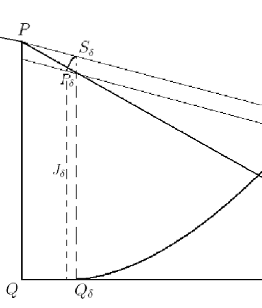
Figure 7: Constructing the curve $l^{i,\varepsilon,\delta}$: a detailed view.

If $x_{i}^{\delta}\geq x_{i}$, the curve $l^{i,\varepsilon,\delta}$ is the union (listed in the consecutive order) of the segments $PS_{\delta}$ and $S_{\delta}S_{\delta}^{\prime}$, the arc $\pi_{\delta}$, the segments $J_{\delta}$ and $Q_{\delta}^{\prime}Q_{\delta}$, and the part of $\Pi_{\delta}$ located to the left of the line $P^{\prime}S$.

If $x_{i}^{\delta}<x_{i}$, the definition of $l^{i,\varepsilon,\delta}$ is more complicated. Define the homothety with the center at $P^{\prime}$ that sends $P$ to $P_{\delta}^{\prime}$, and define the curve $\tilde{l}^{i,\varepsilon,\delta}$ by the following conditions:  (i) the intersection of $\tilde{l}^{i,\varepsilon,\delta}$ with the strip region $x_{i-1}\leq x\leq x_{i}^{\delta}$ is the union of $PS_{\delta}$,  $S_{\delta}S_{\delta}^{\prime}$,  $\pi_{\delta}$,  $J_{\delta}$,  $Q_{\delta}^{\prime}Q_{\delta}$,  $\Pi_{\delta}$, and the interval $\bar{P}_{\delta}P_{\delta}^{\prime}$;  (ii) under the homothety, the curve $\tilde{l}^{i,\varepsilon,\delta}$ moves into itself. The curve $\tilde{l}^{i,\varepsilon,\delta}$ is uniquely defined by these conditions; it does not have self-intersections and connects the points $P$ and $P^{\prime}$. However, it is not piecewise smooth, since it has infinitely many singular points near $P^{\prime}$. In order to improve the situation, define the piecewise smooth curve $l^{i,\varepsilon,\delta}$ in the following way: in the strip $x_{i-1}\leq x<x_{i}-\delta$, it coincides with $\tilde{l}^{i,\varepsilon,\delta}$, the intersection of $l^{i,\varepsilon,\delta}$ with the strip $x_{i}-\delta<x\leq x_{i}$ is the horizontal interval $x_{i}-\delta<x\leq x_{i}$, $z=f_{\varepsilon}(x_{i})$, and the intersection of $l^{i,\varepsilon,\delta}$ with the vertical line $x=x_{i}-\delta$ is a point or a segment (or maybe the union of a point and a segment) chosen in such a way that the resulting curve $l^{i,\varepsilon,\delta}$ is continuous.

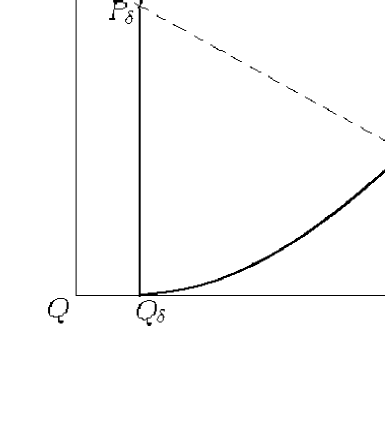
Figure 8: The curve $l^{i,\varepsilon,\delta}$, again.

The particles of the flow falling on the arc $\Pi_{\delta}$ make a reflection from it, pass through the focus $P_{\delta}$, then make another reflection from the arc $\pi_{\delta}$, and finally move freely, the velocity being parallel to $l$. Choose $\delta<|f_{\varepsilon}^{\prime}(0^{+})|$ and $\delta<\min_{1\leq i\leq m-1}(f_{\varepsilon}^{\prime}(x_{i-1}+0)-f_{\varepsilon}^{\prime}(x_{i}+0))$, then the particles after the second reflection will never intersect the other curves $l^{j,\varepsilon,\delta}$,  $j\neq i$. Thus, for the corresponding values of $x$, the vertical component of the velocity of the reflected particle is

$$v^{z}_{G_{\varepsilon,\delta}}(x)=\frac{f^{\prime}_{\varepsilon}(x_{i-1}+0)+\delta}{\sqrt{1+(f^{\prime}_{\varepsilon}(x_{i-1}+0)+\delta)^{2}}}=\hat{v}^{z}_{G_{\varepsilon}}(x)+O(\delta),\leavevmode\nobreak\ \leavevmode\nobreak\ \leavevmode\nobreak\ \delta\to 0^{+}.$$ (30)

If $x_{i}^{\delta}\geq x_{i}$, the formula (30) is valid for $x\in[x_{i-1}+\delta,\,x_{i}]$. If $x_{i}^{\delta}<x_{i}$, it is valid for the values $x\in[x_{i-1}+\delta,\,x_{i}^{\delta}]$. Note, however, that (30) is also valid for values of $x$ that belong to the iterated images of $x\in[x_{i-1}+\delta,\,x_{i}^{\delta}]$ under the homothety, but do not belong to $[x_{i}-\delta,\,x_{i}]$. Summarizing, (30) is true for $x\in[x_{i-1},\,x_{i}]$, except for a set of values of measure $O(\delta)$. Thus, taking into account (26),  (27),  (29), and (30), the convergence (28) is proved. Q.E.D.

3.3 Proof of theorem 2

Let us first state (without proof) the following lemma.

Lemma 3.

Let $\lambda>0$ and let the function $f\in{\mathcal{F}}_{h}$ satisfy the condition

$\mathbf{I}_{\lambda}$.  $f(1)=h$, and for almost all $x\in[0,\,1]$ the value $u=f^{\prime}(x)$ is a solution of the problem

$$xp(u)+\lambda u\rightarrow\min,\quad u\in{\mathbb{R}}_{+}.$$ (31)

Then the function $f$ is a solution of the problem (11) and any other solution satisfies the condition $\mathrm{I}_{\lambda}$ with the same value of $\lambda$.

This simple lemma is a direct consequence of the Pontryagin maximum principle. Its proof can be found, for example, in [13] or in [14].

Now we shall find the function $f_{h}$ satisfying the condition $\mathrm{I}_{\lambda}$ for some positive $\lambda$. Let $x\in[0,\,1]$ be the value for which $\mathrm{I}_{\lambda}$ is fulfilled. Then the value $u=f^{\prime}_{h}(x)$ is also a minimizer for the function $x\bar{p}(u)+\lambda u$, and $p(u)=\bar{p}(u)$. This implies that (if the function $f_{h}$ really exists then)

$$\mathcal{R}[f_{h}]=\int_{0}^{1}\bar{p}(f^{\prime}_{h}(x))\,x\,dx.$$ (32)

Besides, if $u>0$ and $\bar{p}$ is differentiable at $u$ then one has $\frac{d}{du}(x\bar{p}(u)+\lambda u)=0$, hence

$$\frac{x}{\lambda}\ =\ -\frac{1}{\bar{p}^{\prime}(u)}\,.$$ (33)

If $u>0$ and $\bar{p}$ is not differentiable at $u$, then it has left and right derivatives at this point and

$$-\frac{1}{\bar{p}^{\prime}(u-0)}\ \leq\ \frac{x}{\lambda}\ \leq\ -\frac{1}{\bar{p}^{\prime}(u+0)}\,.$$ (34)

If, finally, $u=0$ then one has

$$\frac{x}{\lambda}\ \leq\ -\frac{1}{\bar{p}^{\prime}(0)}\ =\ \xi_{0}.$$ (35)

Put $z=1/\lambda$ and $x_{0}=\xi_{0}/z$ and rewrite (33) and (34) in terms of the generalized inverse function: $\upsilon(zx-0)\leq u\leq\upsilon(zx)$; thus the equality

$$u\ =\ \upsilon(zx),$$ (36)

is valid for almost all values $x\geq x_{0}$. Taking into account (35), substituting $u=f^{\prime}_{h}(x)$, and integrating both parts of (36) with respect to $x$, one comes to (12). In particular, $f_{h}^{\prime}(x_{0}+0)=\upsilon(\xi_{0}+0)=u_{0}$. Using that $f_{h}(1)=h$, one gets (13).

The function $\Upsilon(z)/z$ is continuous and monotone increasing; it is defined on $[\xi_{0},+\infty)$ and takes the values from 0 to $+\infty$. Therefore the equation (13) uniquely defines $z$ as a continuous monotone increasing function of $h$; in particular, $z(0)=\xi_{0}$ and $x_{0}(0)=\xi_{0}/z(0)=1$. The relations (12) and (13) define the function $f_{h}$ solving the minimization problem (11). From the construction one can see that this function is uniquely defined.

Recall that $\mathcal{R}(h)=\mathcal{R}[f_{h}]$. Integrating by parts the right hand side of (32), one gets

$$\mathcal{R}(h)\ =\ \frac{\bar{p}(f_{h}^{\prime}(1))}{2}\ -\ \int_{0}^{1}\,\frac{\ x^{2}}{2}\ \bar{p}^{\prime}(f_{h}^{\prime}(x))\,df_{h}^{\prime}(x).$$

Taking into account that $f_{h}^{\prime}(1)=\upsilon(z)$ and $x\bar{p}^{\prime}(f_{h}^{\prime}(x))=-\lambda=-1/z$, one obtains

$$\mathcal{R}(h)\ =\ \frac{\bar{p}(\upsilon(z))}{2}\,+\,\frac{1}{2z}\,\int_{0}^{1}x\,df_{h}^{\prime}(x),$$

and integrating by parts once again, one gets (14). Substituting in (14) $h=0$ and using that $z(0)=\xi_{0}$,  $\upsilon(\xi_{0})=u_{0}$,  $\Upsilon(\xi_{0})=0$, one obtains $\mathcal{R}(0)=(\bar{p}(u_{0})+u_{0}/\xi_{0})/2$, and using that $p(0)-\xi_{0}^{-1}u_{0}=\bar{p}(u_{0})$, one obtains $\mathcal{R}(0)=p(0)/2$.

Taking into account the asymptotic of $\bar{p}\,$ (which is the same as the asymptotics of $p$:  $\bar{p}(u)=c\,u^{-\alpha}(1+o(1))$,  $u\to+\infty$), and the asymptotic of $\bar{p}^{\prime}$:  $\bar{p}^{\prime}(u)=-c\alpha\,u^{-\alpha-1}(1+o(1))$,  $u\to+\infty,\,$ one comes to the formulas

$$\upsilon(\xi)\,=\,(C\alpha)^{\frac{1}{\alpha+1}}\,\xi^{\frac{1}{\alpha+1}}\,(1+o(1)),\leavevmode\nobreak\ \leavevmode\nobreak\ \leavevmode\nobreak\ \xi\to+\infty,$$

$$\Upsilon(z)\,=\,\left(\frac{\alpha+1}{\alpha+2}\right)(c\alpha)^{\frac{1}{\alpha+1}}\,z^{\frac{\alpha+2}{\alpha+1}}\,(1+o(1)),\leavevmode\nobreak\ \leavevmode\nobreak\ \leavevmode\nobreak\ z\to+\infty,$$

and

$$z\,=\,\frac{1}{c\alpha}\left(\frac{\alpha+2}{\alpha+1}\right)^{\alpha+1}\,h^{\alpha+1}\,(1+o(1)),\leavevmode\nobreak\ \leavevmode\nobreak\ \leavevmode\nobreak\ h\to+\infty.$$

Substituting them into (14) and using the relation $x_{0}=\xi_{0}/z$, after a simple algebra one obtains (16) and (15). The theorem is proved.

Summarizing, the three-dimensional bodies of revolution minimizing the resistance are constructed as follows. First, we find the function $f_{h}^{\text{n}c}$ minimizing the functional (10) and define the convex set $-1\leq x\leq 1$,  $0\leq z\leq h-f_{h}^{\text{n}c}(|x|)$. Next, the upper part of its boundary (which is the graph of the function $z=h-f_{h}^{\text{n}c}(|x|)$) is approximated by a broken line and then substituted with a curve with rather complicated behavior, according to lemma 2. The set bounded from above by this curve is "almost convex": it can be obtained from a convex set by making small hollows on its boundary. By rotating it around the axis $Oz$, one obtains the body of revolution $B$ having nearly minimal resistance $\mathrm{R}_{z}(B)$.

The vertical central cross sections of optimal bodies in the Newton, single impact, and nonconvex cases, for $h=0.8$, are presented on figure 9.

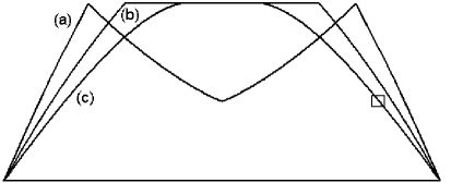
Figure 9: Profiles of optimal solutions in the single impact (a), Newton (b), and nonconvex (c) cases, for $h=0.8$. In the nonconvex case, the profile is actually a zigzag curve with very small zigzags, as shown on the next figure.

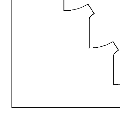
Figure 10: Detailed view of the zigzag curve.

3.4 Derivation of the asymptotic relations in the single impact case

For $h$ small (namely, $h<M^{*}\approx 0.54$), a solution in the single impact case can be described as follows. There are marked several values $-1<x_{-2n+1}<x_{-2n+2}<\ldots<x_{2n-2}<x_{2n-1}<1$,  $n\geq 2$ related to the singular points of the solution. As $h\to 0^{+},\ n=n(h)$ goes to infinity. One has $x_{-k}=-x_{k}$ and $x_{2i}=(x_{2i-1}+x_{2i+1})/2$; thus $x_{0}=0$. Besides, one has $\max_{k}(x_{k}-x_{k-1})=x_{1}=4h/3$. The vertical central cross section of the solution $G=G^{\text{s}i}_{h}\subset{\mathbb{R}}^{2}_{x,z}$ is bounded from above by the graph of a continuous non-negative piecewise smooth even function $f=f_{h}^{\text{s}i}$, and from below, by the segment $-1\leq x\leq 1$,  $z=0$. This function has singularities at the points $x_{k}$, and the values of the function at the points $x_{2i-1}$ coincide: $f(x_{2i-1})=h$. On each interval $[x_{2i-1},\,x_{2i}]$, the graph of $f$ is the arc of parabola with vertical axis and with the focus at $(x_{2i+1},h)$. Similarly, on $[x_{2i},\,x_{2i+1}]$ the graph of $f$ is the arc of parabola with vertical axis and with the focus at $(x_{2i-1},h)$. The first parabola contains the focus of the second one, and vice versa. From this description one can see that on $[x_{2i-1},\,x_{2i}]$, the function equals $f(x)=\frac{(x-x_{2i+1})^{2}}{2(x_{2i+1}-x_{2i-1})}+y_{i}$, and on $[x_{2i},\,x_{2i+1}]$,  $f(x)=\frac{(x-x_{2i-1})^{2}}{2(x_{2i+1}-x_{2i-1})}+y_{i}$, where $y_{i}=h-(x_{2i+1}-x_{2i-1})/2$. On the intervals $[-1,\,x_{-2n+1}]$ and $[x_{2n-1},\,1]$ the graph of the function represents the so-called "Euler part" of the solution (see [8]).

Note that the solution is not unique. The values $x_{1}$ and $x_{2n-1}$ are uniquely determined, but there is arbitrariness in choice of the intermediate values $x_{3},\ldots,x_{2n-3}$ and also in the number $n$ of the independent parameters.

After some calculation, one obtains the value of $1+v_{G}^{z}$ for the figure $G$:

$$\text{if}\leavevmode\nobreak\ \leavevmode\nobreak\ x\in[x_{2i-1},\,x_{2i}],\ \ \ \ \ \ \ 1+v_{G}^{z}(x)\ =\ \frac{2}{1+\left(\frac{x_{2i+1}-x}{x_{2i+1}-x_{2i-1}}\right)^{2}}\leavevmode\nobreak\ ;$$

$$\text{if}\leavevmode\nobreak\ \leavevmode\nobreak\ x\in[x_{2i},\,x_{2i+1}],\ \ \ \ \ \ \ 1+v_{G}^{z}(x)\ =\ \frac{2}{1+\left(\frac{x-x_{2i-1}}{x_{2i+1}-x_{2i-1}}\right)^{2}}\leavevmode\nobreak\ .$$

Let us now calculate the integral $\int_{x_{2i-1}}^{x_{2i+1}}(1+v_{G}^{z}(x))\,x\,dx$,  $1\leq i\leq n-1$. Since the function $1+v_{G}^{z}(x)$,  $x\in[x_{2i-1},\,x_{2i+1}]$ is symmetric with respect to $x=x_{2i}$, the integral equals $2x_{2i}\int_{x_{2i}}^{x_{2i+1}}(1+v_{G}^{z}(x))\,dx$. Changing the variable $t=(x-x_{2i-1})/(x_{2i+1}-x_{2i-1})$ and taking into account that $2x_{2i}=x_{2i-1}+x_{2i+1}$, one comes to the integral $2x_{2i}(x_{2i+1}-x_{2i-1})\int_{1/2}^{1}2/(1+t^{2})\,dt=(x_{2i+1}^{2}-x_{2i-1}^{2})(\pi/2-2\arctan(1/2))$. Therefore

$$\int_{x_{1}}^{x_{2n-1}}(1+v_{G}^{z}(x))\,x\,dx\ =\ (x_{2n-1}^{2}-x_{1}^{2})(\pi/2-2\arctan(1/2)).$$

Taking into account that $x_{1}=4h/3\to 0$ and $x_{2n(h)-1}\to 1$ as $h\to 0^{+}$, one finally gets

$$R(G^{\text{s}i}_{h})\,=\,\int_{0}^{1}(1+v_{G^{\text{s}i}_{h}}^{z}(x))\,x\,dx\,=\,\pi/2-2\arctan(1/2)+o(1),\ \ \ \ \ h\to 0^{+},$$

that is, $\mathcal{R}_{\text{s}i}(0)=\pi/2-2\arctan(1/2)\approx 0.6435$.

If $h>M^{*}$, the function $f=f_{h}^{\text{s}i}$ has three singular points: $x_{1}=x_{1}(h),\ 0$, and $-x_{1}$. On the interval $[-x_{1},\,x_{1}]$, the graph of $f$ is the union of two parabolic arcs, as described above with $i=0$. On the intervals $[-1,\,-x_{1}]$ and $[x_{1},\,1]$, the graph is the "Euler part" of the solution; on both intervals, $f$ is a concave monotone function, with $f(\pm 1)=0$ and $f(\pm x_{1})=h$. The part of resistance of $G=G^{\text{s}i}_{h}$ related to $[0,\,x_{1}]$ can be calculated:

$$\int_{0}^{x_{1}}(1+v_{G}^{z}(x))\,x\,dx\ =\ x_{1}p^{*},$$

where $p^{*}=8(\ln(8/5)+\arctan(1/2)-\pi/4)\approx 1.186$. That is, the convex hull of $G$ represents the solution of the problem (11) with $p(u)=p_{\text{s}i}(u)=\left\{\begin{array}[]{ll}\leavevmode\nobreak\ p^{*}&\text{if }\leavevmode\nobreak\ u=0\\ 2/(1+u^{2})&\text{if }\leavevmode\nobreak\ u>0\leavevmode\nobreak\ \leavevmode\nobreak\ .\end{array}\right.$

References

- [1] I. Newton, Philosophiae naturalis principia mathematica, 1686.
- [2] G. Buttazzo, B. Kawohl, On Newton’s problem of minimal resistance. Math. Intell. 15, No.4, 7-12 (1993).
- [3] G. Buttazzo, V. Ferone, B. Kawohl, Minimum problems over sets of concave functions and related questions. Math. Nachr. 173, 71-89 (1995).
- [4] F. Brock, V. Ferone, B. Kawohl, A symmetry problem in the calculus of variations. Calc. Var. 4, 593-599 (1996).
- [5] G. Buttazzo, P. Guasoni, Shape optimization problems over classes of convex domains. J. Convex Anal. 4, No.2, 343-351 (1997).
- [6] T. Lachand-Robert, M.A. Peletier, Newton’s problem of the body of minimal resistance in the class of convex developable functions. Math. Nachr. 226, 153-176 (2001).
- [7] T. Lachand-Robert, M. A. Peletier. An example of non-convex minimization and an application to Newton’s problem of the body of least resistance. Ann. Inst. H. Poincaré, Anal. Non Lin. 18, 179-198 (2001).
- [8] M. Comte, T. Lachand-Robert, Newton’s problem of the body of minimal resistance under a single-impact assumption. Calc. Var. 12, 173-211 (2001).
- [9] M. Comte, T. Lachand-Robert. Existence of minimizers for Newton’s problem of the body of minimal resistance under a single-impact assumption. J. Anal. Math. 83, 313–335 (2001).
- [10] T. Lachand-Robert and E. Oudet. Minimizing within convex bodies using a convex hull method. SIAM J. Optim. 16, 368–379 (2006).
- [11] A. Yu. Plakhov. Newton’s problem of a body of minimal aerodynamic resistance. Dokl. Akad. Nauk 390, N3, 314–317 (2003).
- [12] A. Yu. Plakhov. Newton’s problem of the body of minimal resistance with a bounded number of collisions. Russ. Math. Surv. 58 N1, 191-192 (2003).
- [13] V. M. Tikhomirov. Newton’s aerodynamical problem. Kvant, no. 5, 11–18 (1982).
- [14] Alexander Plakhov and Delfim Torres. Newton’s aerodynamic problem in media of chaotically moving particles. Sbornik: Math. 196, 885-933 (2005).