Threshold production of meta-stable bound states of Kaluza Klein excitations in Universal Extra Dimensions

Abstract

We study the formation and detection at the next linear $e^{+}e^{-}$ collider of bound states of level-1 quark Kaluza-Klein excitations ${\cal B}_{KK}$ within a scenario of universal extra-dimensions (UED). The interactions of such Kaluza-Klein excitations are modeled by an $\alpha_{s}$ driven Coulomb potential. In order to obtain the threshold cross-section, we employ the Green function method which is known to properly describe the peaks below threshold and to yield a net increase in the continuum region (above threshold) relative to the naive Born cross-section. We study such effect at different values of the scale ($R^{-1}$) of the extra-dimensions with an explicit calculation of the mass spectrum as given by radiative corrections. The overall effect is roughly 2.7 at $R^{-1}=300$ GeV and goes down to $2.2$ at $R^{-1}=1000$ GeV and a relatively large number of events is expected from $N_{events}\approx 2.5\times 10^{4}$ at $R^{-1}=300$ GeV down to $N_{events}\approx 10^{3}$ at $R^{-1}=1000$ GeV at the anticipated annual integrated luminosity of $L_{0}=100$ fb^-1. We finally discuss some potentially observable signatures such as the multilepton channels $2j+2\ell+E\!\!\!\!/$  and $2j+4\ell+E\!\!\!\!/$ for which we estimate statistical significance $\gtrsim 2$ for $R^{-1}$ up to $600\sim 700$ GeV.

I Introduction

It is well known that as early as 1921 Theodore Kaluza proposed a theory that was intended to unify gravity and electromagnetism by considering a space-time with one extra space-like dimension Kaluza:1921tu . A few years later Oscar Klein proposed that the extra space dimension (the fifth dimension) is in reality compactified around a circle of very small radius Klein:1926tv . These revolutionary ideas have thereafter been ignored for quite some time. However recent developments in the field of string theory have suggested again the possibility that the number of space time dimensions is actually different from $D=4$ (indeed string theory models require $D=11$, i.e. seven additional dimensions). In 1990 it was realized Antoniadis:1990ew that string theory motivates scenarios in which the size of the extra dimensions could be as large as $R\approx 10^{-17}$ cm (corresponding roughly to electro-weak energy scale ($\approx$ TeV) contrary to naive expectations which relate them to a scale of the order of the Planck length $L_{P}\approx 10^{-33}$ cm (corresponding to the Planck mass $M_{P}=\sqrt{\hbar c/G}\approx 10^{19}$ GeV). See also Antoniadis:1998ig .

Subsequently two approaches have been developed to discuss the observable effects of these, as yet, hypothetical extra dimensions. One possibility is to assume that the extra space-like dimensions are flat and compactified to a “small” radius. This is the so called ADD model ArkaniHamed:1998rs where only the gravitational interaction is assumed to propagate in the extra-dimension. A second possibility is contemplated in the Randall-Sundrum type of models where the extra dimensions do have curvature and are embedded in a warped geometry Randall:1999ee ; Randall:1999vf .

Universal extra-dimensional models were introduced in ref. Appelquist:2000nn and are characterized, as opposed to the ADD model, by the fact that all particles of the Standard Model (SM) are allowed to propagate in the (flat) extra space dimensions, the so called bulk. Here to each SM particle $X^{(0)}$ corresponds in this model a tower of Kaluza-Klein states $X^{(n)}$ (KK-excitations), whose masses are related to the size of the compact extra dimension introduced and the mass of the SM particle via the relation $m^{2}_{X^{(n)}}\approx m^{2}_{X^{(0)}}+n^{2}/R^{2}$. An important aspect of the UED model is that it provides a viable candidate to the Cold Dark Matter. This would be the lightest KK particle (LKP) which typically is the level 1 photon. Many aspects of the phenomenology of these KK excitations have been discussed in the literature. For reviews see ref. Hooper:2007qk ; Macesanu:2005jx ; Rizzo:2010zf ; Cheng:2010pt . In particular KK production has been considered both at the Cern large hadron collider (LHC) and at the next linear collider (ILC). Direct searches of KK level excitations at collider experiments give a current bound on the scale of the extra-dimension of the order $R^{-1}\gtrsim 300$ GeV. See for example ref. PDBook . At the Fermilab Tevatron it will be possible to test compactification scales up to $R^{-1}\sim 500$ GeV at least within some particular scenario Macesanu:2002db ; Macesanu:2002ew ; Macesanu:2002hg .

Lower bounds on the compactification radius arise also from analysis of electro-weak precision measurements performed at the $Z$ pole (LEP II). An important feature of these type of constraints is their dependence on the Higgs mass. A recent refined analysis Gogoladze:2006br taking into account sub-leading contributions from the new physics as well as two-loop corrections to the standard model $\rho$ parameter finds that $R^{-1}\gtrsim 600$ GeV for a light Higgs mass ($m_{H}=115$ GeV) and a top quark mass $m_{t}=173$ GeV at 90% confidence level (C.L.). Only assuming a larger value of the Higgs mass the bound is considerably weakened down to $R^{-1}\gtrsim 300$ GeV for $m_{H}=600$ GeV, thus keeping the model within the reach of the Tevatron run II. The finding of this precision analysis are in qualitative agreement with previous results Appelquist:2002wb , but are at variance with the conclusions of a recent paper Flacke:2005hb where an analysis of LEP data including data from above the $Z$ pole and two loop electro-weak corrections to the $\Delta\rho$ parameter pointed to $R^{-1}\gtrsim 800$ (at 95% C.L.).

Equally important turn out to be the lower bounds from the inclusive radiative decay $\bar{B}\to X_{s}\gamma$. It has been shown in ref. Haisch:2007vb that a refined analysis including in addition to the leading order contribution from the extra-dimensional KK states, the known next-to-next-to-leading order correction in the Standard model (SM) gives a lower bound on the compactification radius $R^{-1}\gtrsim 600$ GeV at $95\%$ confidence level (CL) and independent of the Higgs mass.

In this work we study the formation, production and possible detection of bound states of Kaluza-Klein $n=1$ excitations at $e^{+}e^{-}$ collisions. The production of bound states of KK excitation has been the object of some previous work Carone:2003ms . As compared to ref. Carone:2003ms where the bound states production rates have been estimated by using a Breit-Wigner approximation, our study makes use of the method of the Green function in order to estimate the bound state contribution at the threshold cross-section, an effect which can be as large as a factor of three when considering strongly interacting particles. In describing the interactions that allow the formation of level-1 KK bound states we assume that the level-1 KK quark excitations interact via an $\alpha_{s}$ driven Coulomb potential. This allows the use of analytic expressions for the Green function of the Coulomb problem but it should be kept in mind that the results and conclusions about formation and decay of the bound state depend on this assumption. This method has also been recently used by the present authors in a study of sleptonium bound states within a slepton co-next to lightest supersymmetric particle (slepton co-NLSP) scenario of gauge mediated symmetry breaking (GMSB) Fabiano:2005gt .

The plan of the paper is as follows. Section II briefly describes the UED model taken as a reference scenario. Section III discusses the formation criteria and shows that the bound states of KK level-1 excitations do indeed form. Section IV describes the Green function method for the bound states providing an analytic formula for the Born production cross section. The threshold cross section for the bound state is studied for several values of the scale of the extra dimension $R^{-1}$. Section V discusses the possible decays of the bound states. Finally in Section VI we discuss the possible observation of the KK bound states at the $e^{+}e^{-}$ linear collider pointing to three possible signatures whose standard model background are also considered providing an estimate of the statistical significance. In section VII we present the conclusions.

II Universal Extra Dimensions

The UED model is constructed considering the Standard Model in a space time of $4+D$ dimensions, and assuming that all SM particles are allowed to propagate in the extra dimensions which typically are assumed to be compactified to a radius $R$. In the following we follow strictly the notation of ref. Hooper:2007qk . We indicate the usual four dimensional coordinates as $x^{\mu}$, $\mu=0,1,2,3$ and with $y^{a},a=1,\cdots D$ the extra space dimensions. The effective four-dimensional Lagrangian is then obtained by dimensional reduction, i.e. by integrating the $4+D$ dimensional SM Lagrangian over the $D$ extra space dimensions. Thus one has:

$${\mathcal{L}}_{eff}(x^{\mu}) = \int\ {\rm d}^{D}y\Big{\{}-\sum_{i=1}^{3}\ \frac{1}{2\hat{g}^{2}_{i}}{\rm Tr}\Big{[}F_{i}^{AB}(x^{\mu},y^{a})F_{iAB}(x^{\mu},y^{a})\Big{]}+$$ (1)

$$+\left|(D_{\mu}+D_{3+a})H(x^{\mu},y^{a})\right|^{2}+\mu^{2}H^{*}(x^{\mu},y^{a})H(x^{\mu},y^{a})-\lambda\big{[}H^{*}(x^{\mu},y^{a})H(x^{\mu},y^{a})\big{]}^{2}+$$

$$+i\left(\overline{Q},\overline{u},\overline{d},\overline{L},\overline{e}\right)(x^{\mu},y^{a})\left(\Gamma^{\mu}D_{\mu}+\Gamma^{3+a}D_{3+a}\right)\left({Q},{u},{d},{L},{e}\right)(x^{\mu},y^{a})+$$

$$\Big{[}\overline{Q}(x^{\mu},y^{a})\left(\hat{\lambda}_{u}\ {u}(x^{\mu},y^{a})i\sigma_{2}H^{*}(x^{\mu},y^{a})+\hat{\lambda}_{d}\ {d}(x^{\mu},y^{a})H(x^{\mu},y^{a})\right)+{\rm H.c.}\Big{]}+$$

$$\Big{[}\overline{L}(x^{\mu},y^{a})\hat{\lambda}_{e}\ {e}(x^{\mu},y^{a})H(x^{\mu},y^{a})+{\rm H.c.}\Big{]}.$$

In the above Eq. 1 $F_{i}^{AB}$ are the gauge field strength tensors of SM gauge group $SU(2)\times U(1)\times SU(3)$ and $\hat{g}_{i}$ are the gauge coupling constants in $(4+D)$-dimensions which have dimension of $(mass)^{-D/2}$ as well as the Yukawa couplings $\hat{\lambda}_{u,d,e}$. $D_{\mu}=\partial/\partial x^{\mu}-\mathcal{A}_{\mu}$ and $D_{a}=\partial/\partial y^{a}-\mathcal{A}_{3+a}$ are the covariant derivative and $\mathcal{A}_{A}=-i\sum_{k=1}^{3}\hat{g}_{k}T^{r}_{i}(\mathcal{A}_{A})_{i}^{r}$ are gauge fields. $Q,L$ are the $SU(2)$ doublets, while $u,d,e$ are the singlet $(4+D)$-dimensional fermion fields. $\Gamma^{A},A=0,\cdots(3+D)$ are (4+D)-dimensional gamma matrices satisfying the anti-commutation relations $\{\Gamma^{A},\Gamma^{B}\}=2g^{AB}$. In the following we shall deal with the simplest case of only one extra-dimension ($D=1$) .

In order to extract the four-dimensional effective theory one needs to specify how the extra-dimensions are compactified. It is found that in order to reproduce chiral fermions in 4-dimension (the SM fermions) one is forced to assume an orbifold compactification structure which depends on the number of extra dimensions. For D-odd (e.g. $D=1$) one chooses an $S^{1}/Z_{2}$ orbifold structure with $Z_{2}$ being the reflection symmetry $y\to-y$. One assumes that the gauge fields ${\mathcal{A}}_{\mu}$ and the Higgs boson $H$ are even under the $y\to-y$ transformation, while the ${\mathcal{A}}_{5}$ is assumed odd. This results in a Fourier series expansion of the fields which defines the zero modes (that correspond to the SM particles) and the level-$n$ KK-excitation (coefficients of the expansions).

$$H(x^{\mu},y) = \frac{1}{\sqrt{\pi R}}\Big{[}H^{0}(x_{\mu})+\sqrt{2}\sum_{n=1}^{\infty}H^{n}(x_{\mu})\cos\left(\frac{ny}{R}\right)\Big{]}$$ (2)

$${\mathcal{A}}_{\mu}(x^{\mu},y) = \frac{1}{\sqrt{\pi R}}\Big{[}{\mathcal{A}}_{\mu}^{0}(x_{\mu})+\sqrt{2}\sum_{n=1}^{\infty}{\mathcal{A}}_{\mu}^{n}(x_{\mu})\cos\left(\frac{ny}{R}\right)\Big{]}$$ (3)

$${\mathcal{A}}_{5} = \sqrt{\frac{2}{\pi R}}\sum_{n=1}^{\infty}{\mathcal{A}}_{5}^{(n)}(x_{\mu})\sin\left(\frac{ny}{R}\right).$$ (4)

As already anticipated, difficulties arise when trying to construct chiral fermion fields in more than four dimensions. This is because in $5$-dimensions, for example, it is not possible to construct the equivalent of the $\gamma_{5}$ matrix and bi-linear quantities like $\bar{\psi}\gamma^{\mu}\gamma_{5}\psi$ are not invariant under $5-$dimensional Lorentz transformations and therefore they cannot appear in the $5D$-Lagrangian. This ultimately implies that for each standard model field one must introduce two $5D$ fermion fields whose zeroth order modes combine to give the $4D$ chiral fermion. This however leaves some extra massless degrees of freedom at the zero level which can only be eliminated by formulating the theory on an orbifold Macesanu:2005jx ; Papavassiliou:2001be . The 5-dimensional fermion field is thus expanded as:

$$\Psi(x^{\mu},y) = \frac{1}{\sqrt{\pi R}}\Big{[}\psi^{\rm SM}(x^{\mu})+\sqrt{2}\sum_{n=1}^{\infty}\psi_{L}^{(n)}(x^{\mu})\cos\left(\frac{ny}{R}\right)$$ (6)

$$\phantom{xxxxxxxxxxx}+\psi_{R}^{(n)}(x^{\mu})\sin\left(\frac{ny}{R}\right)\Big{]}.$$

Performing the integration over the extra space dimension the derivatives with respect to $y$ will bring about mass terms that scale with the compactification radius $R$. Every level-$n$ KK excitation $X_{(n)}$ acquires, in addition to the SM mass (level $0$), obtained via the Higgs mechanism, a new term:

$$m^{2}_{X^{(n)}}=m^{2}_{X^{(0)}}+\frac{n^{2}}{R^{2}},$$ (7)

These relations are however modified by radiative corrections which turn out to be cut-off dependent. These radiative corrections arise from loop diagrams traversing the extra-dimension Cheng:2002ab (bulk loops) and from kinetic terms localized on the brane which appear on the orbifold structure.

$$\delta(m^{2}_{B^{(n)}}) = \frac{g^{\prime 2}}{16\pi^{2}R^{2}}\left[\frac{-39}{2}\frac{\zeta(3)}{\pi^{2}}-\frac{n^{2}}{3}\log\,(\Lambda R)\right]$$

$$\delta(m^{2}_{W^{(n)}}) = \frac{g^{2}}{16\pi^{2}R^{2}}\left[-\frac{5}{2}\frac{\zeta(3)}{\pi^{2}}+15n^{2}\log\,(\Lambda R)\right]$$

$$\delta(m^{2}_{g^{(n)}}) = \frac{g_{3}^{2}}{16\pi^{2}R^{2}}\left[-\frac{3}{2}\frac{\zeta(3)}{\pi^{2}}+23n^{2}\log\,(\Lambda R)\right]$$

$$\delta(m_{Q^{(n)}}) = \frac{n}{16\pi^{2}R}\left[6g_{3}^{2}+\frac{27}{8}g^{2}+\frac{1}{8}g^{\prime 2}\right]\log\,(\Lambda R)$$

$$\delta(m_{u^{(n)}}) = \frac{n}{16\pi^{2}R}\left[6g_{3}^{2}+2g^{\prime 2}\right]\log\,(\Lambda R)$$

$$\delta(m_{d^{(n)}}) = \frac{n}{16\pi^{2}R}\left[6g_{3}^{2}+\frac{1}{2}g^{\prime 2}\right]\log\,(\Lambda R)$$

$$\delta(m_{L^{(n)}}) = \frac{n}{16\pi^{2}R}\left[\frac{27}{8}g^{2}+\frac{9}{8}g^{\prime 2}\right]\log\,(\Lambda R)$$

$$\delta(m_{e^{(n)}}) = \frac{n}{16\pi^{2}R}\frac{9}{2}g^{\prime 2}\log\,(\Lambda R)\;.$$ (8)

Here $\zeta(z)$ is the Riemann zeta function, $\zeta(3)\approx 1.2020$, and $\Lambda$ is the cutoff scale of the theory. It correspond to the energy scale at which the effective 5-dimensional theory will break down, that is where the 5-dimensional couplings become strong and the theory is no longer perturbative. $\Lambda$ is the only additional parameter of the UED model beside the size of the extra dimension $R$. It can be estimated requiring that that loop expansion parameters remain perturbative. It has been found that the SU(3) interaction becomes non perturbative before the other gauge interactions for values of $\Lambda\gtrsim 10\,R^{-1}$. So the particle spectrum is typically computed with the above Eq. II taking $\Lambda R=5,10,20$. In the above expressions the brane kinetic terms are those dependent on the cutoff scale $\Lambda$. It should be noted that for KK scalars and spin-1 bosons the corrections in Eq. II simply add to Eq. 7, while the corrections for the fermion masses are introduced via the replacement $n^{2}/R^{2}\to(n/R+\delta m^{(n)})^{2}$.

$R^{-1}$ (GeV)	$KK$ mass (GeV)	$\alpha_{s}(r_{B}^{-1})$	State mass $M$ (GeV)	$E_{1S}$ (GeV)	$\Delta E(2P-1S)$ (GeV)
300	358.54	0.136	714.06	2.937	2.203
400	478.05	0.131	952.57	3.627	2.720
500	597.56	0.127	1190.92	4.279	3.209
600	717.08	0.124	1429.30	4.903	3.677
700	836.60	0.122	1667.69	5.505	4.128
800	956.11	0.120	1906.11	6.089	4.567
900	1075.62	0.118	2144.54	6.658	4.993
1000	1195.14	0.116	2382.98	7.214	5.411

Table 1: Results of Coulombic model for the bound state of the level-1 iso-doublet $U_{1}$ quark. The strong coupling $\alpha_{s}$ is computed at the scale $Q=r_{B}^{-1}$, where $r_{B}=3/(2m\alpha_{s})$ is the Bohr’s radius. For each mass value $m$ the scale $Q=r_{B}^{-1}$ depending itself on $\alpha_{s}$ must be solved numerically from the equation $Q=(2/3)\,m\,\alpha_{s}(Q)$.

III $\mathbf{u_{1}\overline{u}_{1}}$ Bound State Formation

In this section we shall review the possible creation of a bound state of the level-1 $KK$-excitation of the $u$-quark, i.e. a bound state $u_{1}\bar{u}_{1}$. The interaction among two Kaluza–Klein excitations are driven by the QCD interaction, thus bearing no differences with respect to the Standard Model; the strength of the interaction is given by $\alpha_{s}$ computed at a suitable scale Fabiano:1993vx ; Fabiano:1994cz ; Fabiano:1997xh . We shall adopt the same formation criterion stated there, namely that the formation occurs only if the level splitting depending upon the relevant interaction existing among constituent particles is larger than the natural width of the would–be bound state. This translates into the formation requirement

$$\Delta E_{2P-1S}\geq\Gamma$$ (9)

where $\Delta E_{2P-1S}=E_{2P}-E_{1S}$ and $\Gamma$ is the width of the would–be bound state. The latter is twice the width of the single $KK$ quark, $\Gamma=2\Gamma_{KK}$, as each $KK$ quark could decay in a manner independent from the other.

We shall stress that $\Gamma$ bears no resembling to the total decay width of the resonance, as it only includes the single $KK$ decay mode and not the annihilation modes discussed later in sec. V. It represents the minimal energy level spread needed for bound state formation, which allows for the separation among the fundamental and the first excited state. If, and only if, the bound state is formed, then it is possible to discuss its annihilation widths as described in sec. V. In our model $V(\bm{x})$ is given by a Coulombic potential

$$V(r)=-\frac{4\alpha_{s}}{3r}$$ (10)

with $r=|\bm{x}|$, and where $\alpha_{s}$ is the usual QCD coupling constant which has been taken at a suitable scale as described in Fabiano:1993vx ; Fabiano:1994cz . This model has proved to be reliable because of high mass values involved in the problem, and gives the great advantage of having full analytical results. We are thus able to compute its energy levels given by the expression

$$\varepsilon_{n}=-\frac{4}{9}\frac{m\alpha_{s}^{2}}{n^{2}}$$ (11)

and the separation of the first two energy levels is given by

$$\Delta E_{2P-1S}=\frac{1}{3}m\alpha_{s}^{2}$$ (12)

The scale at which $\alpha_{s}$ is evaluated is given by the inverse of Bohr’s radius $r_{B}=3/(2m\alpha_{s})$, the average distance of the constituents of the bound state. Therefore it is found by solving numerically the equation $Q=(2/3)\,m\,\alpha_{s}(Q)$ and it is of order $\mathcal{O}(10\mbox{ GeV})$ for $m\approx 300$ GeV and $\mathcal{O}(100\mbox{ GeV})$ fr $m\approx 1200$ (GeV). The corresponding values of $\alpha_{s}$ are given in Table 1. The mass of the $n$th bound state is given by the expression:

$$M_{n}=2m+\varepsilon_{n}$$ (13)

where $m$ is the mass of the constituent $u_{1}$ quark and $E_{n}$ is given by (11). The wavefunction at the origin, which will be needed in order to compute decay widths, for this particular model is given by the expression

$$|\psi(0)|^{2}=\frac{1}{\pi}\left(\frac{2}{3}m\alpha_{s}\right)^{3}$$ (14)

The obtained results are given in Table 1.

We observe that the bound state energies are of the order of the GeV for this range of $KK$ mass, and that the spreading of the first two bound states raise linearly with $m$.

In order to determine whether the bound state will be formed we shall apply the criterion given in eq.( 9). The $KK$-quark decay widths have been already computed in Carone:2003ms , where it has been shown that their values are at most of the order of 100 MeV, one order of magnitude less than the energy splittings. In this scenario the eq. (9) requirement is always fulfilled, and the bound state is formed for $KK$-quark masses in this investigation range.

IV Green Function

In order to describe the cross–section of a $KK$ bound state in the threshold region we shall use the method of the Green function. We briefly review here the essential features of the mechanism, and refer the reader to the literature for further details we Fabiano:2001cw . We start from the Schrödinger equation which describes the bound state by means of a suitable potential $V(\bm{x})$,

$$\bm{H}\psi=\left(-\frac{\nabla_{\bm{x}}^{2}}{2m}+V(\bm{x})\right)\psi=\mathcal{E}\psi\;,$$ (15)

where $\mathcal{E}$ is the energy eigenvalue of the bound state. The threshold cross–section of this bound state is then proportional to the imaginary part of the $S$ wave Green function of this Schrödinger equation, $\mathcal{G}_{1S}(\bm{x},\bm{y},E)$, where the two constituent particles are sited in $\bm{x},\bm{y}$ and $E$ is the energy offset from the threshold (not to be confused with $\mathcal{E}$),

$$(\bm{H}-E)\mathcal{G}_{1S}(\bm{x},\bm{y},E)=\delta(\bm{x}-\bm{y})$$ (16)

By means of the substitution $E\to E+i\Gamma$ we take into account the finite width of the state.

The cross–section is thus proportional to the expression

$$\sigma\sim Im\left.\left[Tr\frac{\partial}{\partial x_{i}}\frac{\partial}{\partial y_{j}}\mathcal{G}_{1S}(\bm{x},\bm{y},E)\right]\right|_{\bm{x}=0,\bm{y}=0}$$ (17)

the derivative of eq. (17) has a simple expression, as we have

$${\sf Tr}\,\left.\frac{\partial}{\partial{x}_{i}}\,\frac{\partial}{\partial{y}_{j}}\,\mathcal{G}_{1S}(\bm{x},\bm{y},E)\right|_{\bm{x}=0,\bm{y}=0}=9\mathcal{G}_{1S}(0,0,E)\,\,.$$ (18)

Figure 1: Production cross sections of level-1 KK doublet quark bound states $U_{1}\bar{U}_{1}$ as a function of the energy offset from threshold ($\sqrt{s}=2m_{U_{1}}+E$), for values of the scale of the extra-dimension $R^{-1}$ in the range $[300\div 600]$ GeV and a total width of $\Gamma=0.5$ GeV. The continuous line is the Green Function result, the dotted one is the Born approximation given by our analytical formula (Eq. 21). The full circles represent the Born cross section from the CalcHEP Datta:2010us numerical session inlcuding also the annihilation diagrams of $\gamma_{2}$ and $Z_{2}$ whose contribution is however completely negligible. The numerical results from CalcHEP are in complete agreement with our analytical formula in Eq. 21. The cut-off scale $\Lambda$, at which perturbative expansions break down, has been fixed so that $\Lambda R=20$.

Figure 2: Production cross sections of level-1 KK doublet quark bound states $U_{1}\bar{U}_{1}$ as a function of the energy offset from threshold ($\sqrt{s}=2m_{U_{1}}+E$), for values of the scale of the extra-dimension $R^{-1}$ in the range $[700\div 1000]$ GeV and a total width of $\Gamma=0.5$ GeV. The continuous line is the Green Function result, the dotted one is the Born approximation given by our analytical formula (Eq. 21). The full circles represent the Born Cross section from the CalcHEP Datta:2010us numerical session inlcuding also the annihilation diagrams of $\gamma_{2}$ and $Z_{2}$ whose contribution is however completely negligible. The numerical results from CalcHEP are in complete agreement with our analytical formula in Eq. 21. As in Fig. 1 we have kept fixed $\Lambda R=20$.

The complete expression for the $1S$ Green function of our problem as a function of energy from threshold is given with a slight change of notation by Penin:1998mx :

$$\mathcal{G}_{1S}(0,0,E+i\Gamma) = \frac{m}{4\pi}\left[-2\lambda\left(\frac{k}{2\lambda}+\log\left(\frac{k}{\mu}\right)+\right.\right.$$ (19)

$$\left.\left.\phantom{xxx\frac{1}{2}}\,\psi(1-\nu)+2\gamma-1\right)\right]$$

where $k=\sqrt{-m(E+i\Gamma)}$, $\lambda=2\alpha_{s}m/3$ and the wave number is $\nu=\lambda/k$; $E=\sqrt{s}-2m$. The $\psi$ is the logarithmic derivative of Euler’s Gamma function $\Gamma(x)$, $\gamma\simeq 0.57721$ is Euler’s constant and $\mu$ is an auxiliary parameter coming out from a dimensional regularization, the factorization scale, that cancels out in the determination of physical observables.

The final expression for the production cross–section of a $KK$ bound state is thus given by

$$\sigma(m,E,\Gamma,\alpha_{s})=\frac{18\pi}{m^{2}}\sigma_{B}\,\text{Im}\,\left[\mathcal{G}_{1S}\right]$$ (20)

where $\sigma_{B}$ is the Born expression of the cross–section Burnell:2005hm The process $e^{+}e^{-}\to U_{1}\bar{U}_{1}$ proceeds through the annihilation into the standard model (level-0) gauge bosons $\gamma$ and $Z$ but in principle one should also consider the contribution of the level-2 gauge bosons $\gamma_{(2)}$ and $Z_{(2)}$. Especially so in our case of threshold production of the pair $u_{1}\bar{u}_{1}$. Indeed in this case $m\approx 1/R$, and $\sqrt{s}=2m+E\approx 2/R+E$ and since $m_{\gamma_{2}}\approx 2/R$ when producing at threshold the $u_{1}\bar{u}_{1}$ pair we would be close to the $\gamma_{2}$ and $Z_{2}$ resonances. However as discussed in section II the mass spectrum is modified by the radiative corrections. We have verified that over the region of parameter space $300\,\,\text{GeV }\leq R^{-1}\leq 1000\,\,\text{GeV}$ and $2\leq\Lambda R\leq 70$ the pair production threshold $2m_{u_{1}}$ is always larger than $m_{\gamma_{2}},m_{Z_{2}}$ and thus these resonances should in principle be included in the calculation. We have also verified, cross checking our calculation with the output of a CalcHEP Pukhov:2004ca ; Datta:2010us session, that the numerical impact of these diagrams is completely negligible. Their contribution turns out to be five orders of magnitude smaller than that of the SM gauge bosons $\gamma,Z$. The analytic formula of the Born pair production cross section $e^{+}e^{-}\to\gamma^{*},Z^{*}\to U_{1}\bar{U}_{1}$ can be deduced for example from those of heavy quark ($t\bar{t}$) Panella:1993zk taking into account the fact the the level-1 KK quarks are vector-like i.e. their coupling to the $Z$ is of the $\gamma^{\mu}$ type and has no axial component. Following the notation of Panella:1993zk the amplitude is written as:

$${\cal M} = g_{V}^{2}\sum_{V=\gamma,Z}\bar{v}(k_{2})\gamma^{\mu}(a_{V}+b_{V}\gamma^{5})u(k_{1})\times$$

$$\frac{1}{D_{V}(s,M_{V})}\,\bar{u}(p_{1})\gamma_{\mu}(A_{V}+B_{V}\gamma^{5})v(p_{2})$$

where $D_{V}(s)=s-M_{V}^{2}+iM_{Z}\Gamma_{Z}$ is the gauge boson propagator factor, $a_{V},b_{V}$ are the (standard model) coupling coefficients of the electron to the gauge bosons while $A_{V},B_{V}$ are the coupling coefficients of the level-1 KK $U_{1}$ quark to the gauge bosons. These electron coefficients are: $a_{\gamma}=-1$, $b_{\gamma}=0$, $a_{Z}=-1/4+\sin^{2}\theta_{W}$, $b_{Z}=+1/4$, with $\theta_{W}$ the Weinberg angle of the $SU(2)\otimes U(1)$ gauge theory. The $U_{1}$ coefficients are: $A_{\gamma}=+2/3$, $A_{Z}=1/2-(2/3)\sin^{2}\theta_{W}$ Hooper:2007qk , $B_{\gamma}=B_{Z}=0$ (recall that $U_{1}$ is vector-like). Finally $g_{\gamma}=e$ and $g_{Z}=e/(\cos\theta_{W}\sin\theta_{W})$ with $e$ the electronic charge. The final expression of the Born pair production cross section is:

$$\sigma_{B} = \sigma_{\gamma}+\sigma_{Z}+\sigma_{{\gamma}Z}$$ (21)

$$\sigma_{\gamma} = \frac{16\pi\alpha^{2}}{9s^{2}}\beta(s+2m^{2})$$ (22)

$$\sigma_{Z} = {4\pi\alpha^{2}}\,\frac{(a_{Z}^{2}+b_{Z}^{2})A_{Z}^{2}}{[c_{w}^{2}s_{w}^{2}]^{2}}\,\frac{\beta(s+2m^{2})}{|D_{Z}(s)|^{2}}$$ (23)

$$\sigma_{\gamma Z} = -8\pi\alpha^{2}\frac{a_{Z}A_{\gamma}A_{Z}}{c_{w}^{2}s_{w}^{2}}\,\frac{\beta(s+2m^{2})}{|D_{Z}(s)|^{2}}(1-\frac{M_{Z}^{2}}{s})$$ (24)

where $c_{W}=\cos\theta_{W}$ and $s_{W}=\sin\theta_{W}$ and $\alpha=e^{2}/(4\pi)$ is the QED fine structure constant. From Eq. (19) one can readily see the behavior of the cross–section (20) for large $E$ is given by $k$. The finite width of the state has been taken into account by the substitution $E\to E+i\Gamma$, and this position makes a great quantitative difference below threshold. When computed for positive energy offset the variation of $\Gamma$ makes essentially no difference for the resulting cross–section.

In this work we shall concentrate on the continuum region of the cross–section, namely $E>0$. The region below threshold, $E<0$, has been already discussed in detail in ref. Carone:2003ms , where the authors presented an analysis of both the positions and the widths of the peaks using a Breit-Wigner description. In this respect the Green function approach does not carry substantial differences relative to the Breit–Wigner one. Indeed the position of the poles and the broadening of the peaks are the same due to the presence, inside the $\psi$ function of Eq. (19), of terms which include the binding energy $E_{n}$ of Eq. (11) and the decay width $\Gamma$. For values of $E$ close to $E_{n}$, the argument of the $\psi$ function inside Eq. (19), namely $(1-\nu)$, approaches a negative integer, simple pole of the function in the complex plane, while the presence of the $\Gamma$ determines the width of the peak centered in $E_{n}$.

In Fig. 1 we show the cross–section for a range of the value of the scale of the extra dimension, $R^{-1}=300-600$ GeV, while Fig. 2 provides the same plots are shown the range $R^{-1}=700-1000$ GeV. In both figures the value of the other parameter is fixed at $\Lambda R=20$. This parameter enters our calculations only when computing the mass spectrum through the logarithmic terms in Eq. II. We thus provide a quantitative study of the effect of the formation of bound states of the level-1 KK quarks with respect to the parameter of the model ($R^{-1}$). The results are less sensitive to the other parameter ($\Lambda R$) which only enters through the logarithmic factors in the radiative correction terms in the mass spectrum of the model. In Figs. 1& 2 we have fixed $\Lambda R=20$ and varied $R^{-1}$ computing the corresponding values of the level-1 KK quark mass, and assuming the energy of the collider being fixed at $\sqrt{s}=2m_{U_{1}}+E$, $E$ being the energy offset from the threshold. We have used a value of $\Gamma=0.5$ GeV for illustrative purpose, compatible with the formation of bound state. Different choices of $\Gamma$ by even two orders of magnitude smaller will not make a visible difference on the figures.

One can observe that the cross–section obtained by the Green function has a behavior like $\sqrt{E}$ for small energy offset. The cross–section decreases with increasing mass: for $E=10$ GeV its value is about 250 fb at $R^{-1}=300$ GeV, goes down to approximately 70 fb at $R^{-1}=500$ GeV. Finally it approaches 13 fb at $R^{-1}=1000$ GeV as can be seen form Fig. 2. The Green function cross section is larger than the Born cross-section by a factor that ranges from 2.7 (at $R^{-1}=300$ GeV) down to 2.2 (at $R^{-1}=1000$ GeV) at the same energy offset value ($E=10$ GeV). This result is due to the fact that the Green function method takes into account the existing interaction among constituent particles, and the contribution of binding energies accumulate towards the $\varepsilon=0$ level, thus substantially contributing to the continuum region as well.

An important consideration is in order here. The results for the bound state cross–section given depend solely on the coupling constant $\alpha_{s}(r_{B})$ and the mass of the $KK$ excitation, thus they are universal to bound states made out of other flavors of $KK$ quarks. This however does not apply to other kinds of $KK$ excitations bound states, like for instance bound states of KK-leptons. In this case we have $\alpha\equiv\alpha_{QED}$ for coupling constant, much weaker at this scale than the strong coupling constant $\alpha_{s}(r_{B})$. The QED coupling constant would lead, not only to lower values for the absolute production cross-section, but will also reduce drastically the main effect being discussed here, i.e. the enhancement, above threshold, due to the bound state interaction relative to the Born cross-section. The threshold cross-section would be only a few percent larger than the Born cross-section. It would not clearly be an effect as large as that shown in figs (1), (2) which turns out to be quite striking, i.e. the threshold bound-state cross section is about three times as large as the Born result.

V $\mathbf{u_{1}\overline{u}_{1}}$ Decay Widths

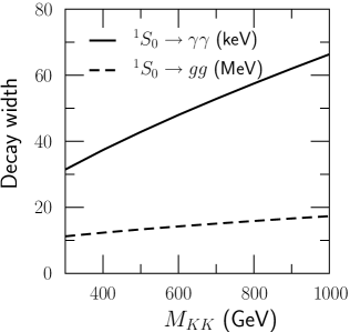
Figure 3: Solid line: decay width (keV) of the pseudoscalar $u_{1}\bar{u}_{1}$ bound state to two photons as a function of $KK$ excitation mass. Dashed line: decay width (MeV) of the pseudoscalar $u_{1}\bar{u}_{1}$ bound state to two gluons as a function of the $KK$ mass.

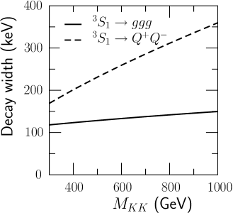
Figure 4: Decay widths of the $u_{1}\bar{u}_{1}$ vector bound state to two charged particles and into three gluons as a function of $KK$ mass. Here we have considered all possible e.m. decay channels.

The $KK$ bound states we discuss here are the pseudoscalar ${}^{1}S_{0}$ and the vector one ${}^{3}S_{1}$. For the pseudoscalar state the decay channels are into two photons or two gluons for which the following Born level expressions hold (see for instance Fabiano:1994cz ):

$$\Gamma_{B}(^{1}S_{0}\to\gamma\gamma)=q_{i}^{4}\alpha^{2}\frac{48\pi|\psi(0)|^{2}}{M^{2}}$$ (25)

and

$$\Gamma_{B}(^{1}S_{0}\to gg)=\alpha_{s}^{2}\frac{32\pi|\psi(0)|^{2}}{3M^{2}}\;.$$ (26)

Here $q_{i}$ is the charge of the constituent quark of the bound state, while $M$ and $|\psi(0)|^{2}$ are given by (13) and (14) respectively.

The QCD radiative correction Kwong:1987ak , which is the same in the two cases, lead to the following one-loop width:

$$\Gamma=\Gamma_{B}\left[1+\frac{\alpha_{s}}{\pi}\left(\frac{\pi^{2}-20}{3}\right)\right]$$ (27)

The results obtained for the two decays ${}^{1}S_{0}\to\gamma\gamma$ and ${}^{1}S_{0}\to gg$ are shown in Fig. 3.

For the vector case ${}^{3}S_{1}$ the relevant decay channels are the one in charged pairs and the one into three gluons, for which one has

$$\Gamma_{B}(^{3}S_{1}\to q_{f}^{+}q_{f}^{-})=q_{i}^{2}q_{f}^{2}\alpha^{2}\frac{16\pi|\psi(0)|^{2}}{M^{2}}$$ (28)

and

$$\Gamma_{B}(^{3}S_{1}\to ggg)=\frac{(\pi^{2}-9)}{\pi}\alpha_{s}^{3}\frac{160\pi|\psi(0)|^{2}}{81M^{2}}$$ (29)

The charge of the final state charged particle is given by $q_{f}$. The QCD radiative corrections Kwong:1987ak modify these expressions into

$$\Gamma(^{3}S_{1}\to q_{f}^{+}q_{f}^{-})=\Gamma_{B}(^{3}S_{1}\to q_{f}^{+}q_{f}^{-})\left(1-\frac{16}{3}\frac{\alpha_{s}}{\pi}\right)$$ (30)

and

$$\Gamma(^{3}S_{1} \to ggg)=\Gamma_{B}(^{3}S_{1}\to ggg)\times$$

$$\times\left\{1+\displaystyle\frac{\alpha_{s}}{\pi}\left[-14+\frac{27}{2}\left(1.161+\log(2)\right)\right]\right\}$$

Observe that the $\alpha_{s}$ that appears in the perturbative corrections has to be computed at a scale of the order of $2m$. It is thus different from the $\alpha_{s}$ occurring in the expression of the wavefunction at the origin given by (14), the latter being computed at the scale of the inverse of Bohr radius.

The two decays of the vector state are shown together in Fig. 4.

We observe that only the pseudoscalar hadronic decay is in the MeV range and raises approximately linearly with $KK$ mass. The ${}^{1}S_{0}$ photonic decay and ${}^{3}S_{1}$ decays are smaller by almost two orders of magnitude for the considered $KK$ mass range. For the pseudoscalar case the hadronic is the dominant decay by far, while in the vector case the decay into charged particles, when taking into account all possible processes as seen in Fig. 4 overtakes the hadronic decays.

Other electro-weak decay channels are negligible. Those are proportional to $\alpha^{2}$, thus their ratio to gluonic decays is suppressed by $(\alpha/\alpha_{s})^{2}$, at least by two orders of magnitude.

For most scenarios depending upon the values of $\Lambda$ and $R$ Carone:2003ms single quark decay becomes the dominant decay channel for the bound state.

Any two–body decay width of the bound state is proportional to $g^{2}|\psi(0)|^{2}/M^{2}$, where $g$ is the relevant coupling to the decay particles. Thus any electro-weak width is in the keV range, as previously seen. This result is true in general for any two–body decay process, the only notable exception being the hadronic decay of (26), as the $g$ coupling this time is rather large, being equal to $\alpha_{s}$. In this case the value is in the MeV range, as seen in Fig. 3.

Three–body decays are further suppressed with respect to previous formula by another power in $g$ and phase–space reduction, resorting again in the keV range of energies.

From Carone:2003ms one sees that in most cases single quark decays (SQD) are by far the most important decay channels of the bound state, to the order of hundreds of MeV, while as discussed above bound state decays are essentially negligible. Moreover a comparison of those SQD widths with the results of Table 1 through eq. (9) shows that for the considered mass range of $KK$ there is formation of the bound state.

VI Detection

As we have previously seen, for large $R^{-1}$ values ($R^{-1}>300$ GeV) SQD is the dominant decay channel for a $KK$ bound state, thus leading a to a dominant signature consisting of two monochromatic quarks plus missing energy. Other interesting signatures that could be considered, for example the three jet production due to the bound state decay into three gluons ${}^{3}S_{1}\to ggg$ discussed in the previous section, are clearly subdominant given the fact that ${\cal B}(^{3}S_{1}\to ggg)\approx 10^{-3}$ . Such signatures, in addition would have to be confronted with important QCD backgrounds. Therefore in the following discussion we concentrate on the dominant channels given by the single quark decay whose branching fractions, on the contrary, can be as high as 65% and 98% and involve missing energy in the final state. Following Fabiano:2001cw we limit our analysis to the region above threshold, i.e. $E>0$. The region below threshold, $E<0$, is characterized by peaks in the cross section for values of $E$ equal to binding energies of the bound states. The width of those peaks are given by the decay width of the bound state, which are at most of the order of the MeV for the SQD and much less, of the order of the keV, for other annihilation decay modes, as discussed in sect. V.

From Eq. (11) we can estimate the separation of the various peaks below threshold, which tend to merge when they accumulate, that is for $n$ such that

$$\frac{4}{9}m\alpha_{s}^{2}\left[\frac{1}{n^{2}}-\frac{1}{(n+1)^{2}}\right]\sim\Gamma$$ (32)

in this manner we estimate that the last resolved peak has a quantum number $n$ that satisfies

$$\frac{2n+1}{n^{2}(n+1)^{2}}\sim\frac{9\Gamma}{4m\alpha_{s}^{2}}=\frac{\Gamma}{E_{1}}\ll 1$$ (33)

from the values Table 1 and using a width value of the order of 20 MeV there are only around 5 peaks left before merging.

Because of ISR and beam energy spread, of the order of the GeV for a future linear collider, it is unclear whether it could be possible to resolve those peaks of keV magnitude with this machine. The only potentially detectable peaks should be the ones belonging to a SQD, provided one has a scenario with widths of the order of the MeV.

The situation above threshold changes drastically with respect to the “naive” Breit–Wigner estimate, as is clearly shown in Fig. 1 and Fig. 2 . A few GeV above threshold make for a factor of 3 of increase compared to the Born cross–section, allowing a clear distinction between the two cases. Assuming an annual integrated luminosity of $L_{0}=100$ fb^-1 and a scale of the extra-dimension $R^{-1}=300$ GeV one finds around $2.5\times 10^{4}$ events per year of two quark decay for a center of mass energy of 10 GeV above threshold (we adopt here the scenario for which the branching ratio of SQD is essentially 1). The number of events per year loses an order of magnitude at $R^{-1}=700$ GeV, that is about $3\times 10^{3}$, as could be inferred from Fig. 2.

As we have already said the decay width of the $KK$ bound state will be given by twice the decay of the single quark, as the SQD dominates, being of the order of up to hundreds of MeV. For our $\overline{u}_{1}u_{1}$ bound state there are two possible scenarios of decay pattern Cheng:2002ab . The first one concerns the iso-singlet $u_{1_{R}}$ for which the decay channel into $W_{1}$ is forbidden while that into $Z_{1}$ is heavily suppressed ${\cal B}(u_{1_{R}}\to Z_{1}u_{0_{R}})\sim\sin^{2}\theta_{1}\approx 10^{-2}\div 10^{-3}$ and the dominant channel is given by $u_{1_{R}}\to u_{0_{R}}\gamma_{1}$, with ${\cal B}(u_{1_{R}}\to u_{0_{R}}\gamma_{1})\approx 0.98$ whose signature is a monochromatic quark and missing energy of the $KK$ photon, the latter being the LKP Cheng:2002ab .

For the iso-doublet $u_{1_{L}}$ the situation is more interesting, as more channels are available Cheng:2002ab , notably $u_{1_{L}}\to d_{0_{L}}W_{1}$ with ${\cal B}(u_{1_{L}}\to d_{0_{L}}W_{1})\approx 0.65$ and $u_{1_{L}}\to u_{0_{L}}Z_{1}$, with ${\cal B}(u_{1_{L}}\to u_{0_{L}}Z_{1})\approx 0.33$ while the branching ratio into $\gamma_{1}$ is negligible ${\cal B}(u_{1_{L}}\to u_{0_{L}}\gamma_{1})\sim 0.02$. The decay chain into $W_{1}$ can follow the scheme: $u_{1_{L}}\to d_{0_{L}}W_{1}\to d_{0_{L}}\ell_{0}\nu_{1_{L}}\to d_{0_{L}}\ell_{0}\nu_{0}\gamma_{1}$ with branching ratio given by:

$${\cal B}(u_{1_{L}}\to d_{0_{L}}\ell_{0}\nu_{0}\gamma_{1}) \approx {\cal B}(u_{1_{L}}\to d_{0_{L}}W_{1}){\cal B}(W_{1}\to l_{0}\nu_{1})$$ (34)

$$\times{\cal B}(\nu_{1}\to\nu_{0}\gamma_{1})$$ (35)

$$\approx 0.65\times 1/6\times 1\approx 10^{-1}$$ (36)

and alternatively, the same final state could be reached by the scheme: $u_{1_{L}}\to d_{0_{L}}W_{1}\to d_{0_{L}}\ell_{1}\nu_{0_{L}}\to d_{0_{L}}\ell_{0}\nu_{0_{L}}\gamma_{1}$. As compared to the iso-singlet case, the result is a monochromatic quark, a lepton and missing energy in both cases.

The decay into the $Z_{1}$ channel is $u_{1_{L}}\to u_{0_{L}}Z_{1}\to u_{0_{L}}\ell_{0}\ell_{1}\to u_{0_{L}}\ell_{0}\ell_{0}\gamma_{1}$, resulting in a monochromatic quark, two leptons and missing energy. The branching ratio of the above chain is:

$${\cal B}(u_{1_{L}}\to u_{0_{L}}\ell_{0}\ell_{0}\gamma_{1}) \approx {\cal B}(u_{1_{L}}\to u_{0_{L}}Z_{1}){\cal B}(Z_{1}\to L_{0}L_{1})$$ (37)

$$\times{\cal B}(L_{1}\to\ell_{0}\gamma_{1})$$ (38)

$$\approx \frac{1}{3}\times\frac{1}{6}\times 1\approx 5\times 10^{-2}$$ (39)

These leptonic decays of $u_{1}$ have much cleaner signatures than the hadronic ones allowing, in principle, for a better detection of the signal.

In all cases we emphasize that the observable signal of the bound state production at the linear collider would be similar to that of the Born pair production except for the absolute value of the cross-section. In particular, assuming for definiteness a linear collider operating around the threshold $\sqrt{s}=2m+E$ GeV we would have for $R^{-1}=300$ GeV and $E=10$ GeV, in the case of an iso-singlet bound state (or Born pair production of ${u_{1}}_{R}$):

$$e^{+}e^{-}\to 2\,\textrm{jets}+E\!\!\!\!/$$ (40)

with cross section:

$$\sigma(e^{+}e^{-}\to 2\,\textrm{jets}+E\!\!\!\!/) \approx \sigma_{\cal B_{KK}}\times\left[{\cal B}({u_{1}}_{R}\to u_{0}\gamma_{1})\right]^{2}$$ (41)

$$\approx 173\,\text{fb}.$$ (42)

We note that the $\sigma_{\cal B_{KK}}$ for the iso-singlet $u_{1}$ has to be computed ex-novo and cannot be read from the values of Fig. 1 since it refers to the iso-doublet $U_{1}$. The singlet and doublet have, when including radiative corrections, different masses and the corresponding pair production threshold is therefore different. For the values of the scale of the extra-dimension $R^{-1}=300$ GeV the mass of the $u_{1}$ iso-singlet is $m_{u_{1}}=351.75$ GeV (slightly lighter than the iso-doublet) and the corresponding Green Function cross-section at an energy offset of $E=10$ GeV is $\sigma_{\cal B_{KK}}=181$ fb. At an $e^{+}e^{-}$ collider this signal has a standard model background from $ZZ$ production with one $Z$ decaying to neutrinos and the other decaying hadronically. The cross section for $ZZ$ boson production is $\approx 244$ fb at an energy offset of $E=10$ GeV from the relative thresholds. This provides the following estimate for the SM background at $R^{-1}=300$ GeV:

$$\sigma_{SM}(2\,\textrm{jets}+E\!\!\!\!/)\approx 244\,\text{fb}\times 0.7\times 0.2\approx 34\,\text{fb}$$ (43)

In the case of an iso-doublet bound state (or Born pair production of ${U_{1}}$) the $W_{1}$ decay chain gives the signal:

$$e^{+}e^{-}\to 2\,\textrm{jets}+2\ell+E\!\!\!\!/$$ (44)

with cross section (see Fig. 1):

$$\sigma(e^{+}e^{-}\to 2\textrm{j}+2\ell+E\!\!\!\!/) = \sigma_{{\cal B}_{KK}}\left[{\cal B}(u_{1L}\to d_{0_{L}}\ell_{0}\nu_{0}\gamma_{1})\right]^{2}$$ (45)

$$\approx 275\text{fb}\times(10^{-1})^{2}$$ (46)

$$= 2.75\,\text{fb}$$ (47)

while the $Z_{1}$ decay chain gives rise to the signature:

$$e^{+}e^{-}\to 2\,\textrm{jets}+4\ell+E\!\!\!\!/$$ (48)

with cross sections:

$$\sigma(e^{+}e^{-}\to 2\textrm{j}+4\ell+E\!\!\!\!/) = \sigma_{{\cal B}_{KK}}\left[{\cal B}(u_{1L}\to u_{0_{L}}\ell_{0}\ell_{0}\gamma_{1})\right]^{2}$$ (49)

$$= 275\text{fb}\times(5\times 10^{-2})^{2}$$ (50)

$$\approx 0.69\,\text{fb}$$ (51)

Triple gauge boson production, $WWZ,ZZZ$ at a high energy linear collider has been studied in refs. Barger:1988sq ; Barger:1988fd . It has been found that these processes receive a substantial enanchement in the higgs mass range $200$ GeV $<m_{H}<600$ GeV particularly the $ZZZ$ channel. As these processes provide a source of standard model background for our signal we estimate them both at a value of $m_{h}=120$ GeV and at a value of $m_{h}=200$ GeV for which the cross sections are enhanced. Production of $WWZ$ can for instance give rise to the signature of $2\textrm{jets}+2\ell+E\!\!\!\!/$ via leptonic decay of the W gauge bosons and hadronic decay of the $Z$ boson, while the $ZZZ$ production can produce $2\textrm{jets}+4\ell+E\!\!\!\!/$ via hadronic decay of one $Z$ while the others decay leptonically with one of them to a pair of $\tau$ which subsequently decay to $\ell\nu\bar{\nu}$ ($\ell=e,\mu$). Estimates of the resulting cross sections are found using the CalcHEP Pukhov:2004ca and CompHEP Boos:2004kh software. We have verified agreement with previous results given in ref. Barger:1988fd and for a Higgs mass of $m_{h}=200$ GeV we find, for $R^{-1}=300$ GeV at $\sqrt{s}=2m_{U_{1}}+10\approx 724$ GeV:

$$\sigma(WWZ) \approx 72\,\text{fb}$$ (52)

$$\sigma(ZZZ) \approx \phantom{7}7\,\text{fb}$$ (53)

We thus find at $\sqrt{s}=724$ GeV within the standard model:

$$\sigma_{\text{SM}}(2\textrm{j}+2\ell+E\!\!\!\!/) \approx 70\,\text{fb}\times(0.1)^{2}\times 0.7\approx 0.5\,\text{fb}$$ (54)

$$\sigma_{\text{SM}}(2\textrm{j}+4\ell+E\!\!\!\!/) \approx 7\,\text{fb}\times(0.3)^{2}\times 0.7\times(0.17)^{2}$$ (55)

$$\approx 1.2\times 10^{-2}\,\text{fb}$$ (56)

$R^{-1}$ (GeV)	$m_{u_{1}}$ (GeV)	$2\,\textrm{jets}+E\!\!\!\!/$	$2\,\textrm{jets}+2\,\ell+E\!\!\!\!/$	$2\,\textrm{jets}+4\,\ell+E\!\!\!\!/$
	(iso-singlet)		$m_{h}=120$ GeV (200 GeV)	$m_{h}=120$ GeV (200 GeV)
300	351.7	121.8	13.1 (12.9)	8.3 (8.2)
400	469.0	81.1	8.2 (8.1)	5.6 (5.6)
500	586.2	58.7	5.7 (5.6)	4.2 (4.2)
600	703.5	44.4	4.1 (4.1)	3.3 (3.3)
700	820.7	35.3	3.1 (3.1)	2.7 (2.7)
800	938.0	29.0	2.4 (2.4)	2.3 (2.3)
900	1055.2	24.1	1.9 (1.9)	1.9 (1.9)
1000	1172.5	20.8	1.6 (1.6)	1.7 (1.7)

Table 2: Estimate of the statistical significance $SS$ as defined in Eq. 57 and corresponding to the annual integrated luminosity $L_{0}=100$ fb^-1 for the three channels discussed in the text as a function of $R^{-1}$ and $\sqrt{s}=2m_{U_{1}}+E$, assuming an energy offset of $E=10$ GeV from the threshold. The physical threshold of the $2\,\textrm{jets}+E\!\!\!\!/$ channel is different form that of the other two channels as it refers to the $u_{1}$ iso-singlet level-1 KK quark whose masses at various values of $R^{-1}$ are given in column two and can be compared with the corresponding masses of the $U_{1}$ state form Fig. 1 and Fig. 2. The values of the statistical significance for the two multilepton channels have been computed for two values of the Higgs mass $m_{h}=120\,(200)$ GeV. Again $\Lambda R=20$.

The $2\textrm{jets}+2\ell+E\!\!\!\!/$ channel could be potentially contaminated also from $t\bar{t}$ pair production cross section which at such high energies is ${\cal O}(300)$ fb Weiglein:2004hn . Assuming the top quarks to decay with probability one to $Wb$ and then the $W$ gauge boson decay via the leptonic mode (with ${\cal B}(W\to\ell\nu_{\ell})\approx 0.1$) would mimic the signal with a cross section $\sigma_{SM}(2\textrm{jets}+2\ell+E\!\!\!\!/)\approx 3fb$. However in this case we expect $b$-tagging of the hadronic jets. Assuming an efficiency in $b$-tagging of $60\%$ we would get a contribution of $1.2$ fb to the $2\textrm{jets}+2\ell+E\!\!\!\!/$ cross-section which has to be added to that in Eq. 54. This has been done in the calculation of the statistical significance of table 2.

We conclude providing an estimate of the statistical significance:

$$SS=\frac{N_{\text{s}}}{\sqrt{N_{\text{s}}+N_{\text{b}}}},$$ (57)

of the three signals discussed above as related to an integrated luminosity of $L_{0}=100$ fb^-1 ($N_{\text{s}}$ is the number of signal events and $N_{\text{b}}$ is the number of background events). These estimates are given in table 2 and Fig. 5. Albeit quite encouraging (especially so the $SS$ of the $2\textrm{jets}+E\!\!\!\!/$) we should bear in mind that the actual observation of these signals might be not be so easy from the experimental point of view. Indeed it is quite likely that in a framework of a quasi degenerate KK mass spectrum the jets will be typically quite soft and therefore difficult to detect. It is therefore customary to concentrate on the much cleaner multilepton signatures Cheng:2002ab ; Battaglia:2005zf . Indeed a similar analysis to the one given here, but with a perspective on signals arising at the Compact Linear Collider (CLIC), regarding the (Born) pair-production of level-1 KK-leptons and level-1 KK-quarks is given in ref. Battaglia:2005zf .

It is also well known that jets, multilepton and missing energy signals are as well typical of supersymmetric models. Indeed detailed studies have already appeared in the literature regarding the possibility of distinguishing supersymmetric and universal extra dimension models at both the large hadron collider and linear collider: see for example ref. Datta:2005zs ; Smillie:2005ar ; Freitas:2007rh .

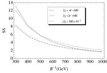
Figure 5: Statistical significance ($SS$) for the various channels discussed in the text as a function of the scale $R^{-1}$ of the extra-dimensions. Note that the statistical significance of the $2j+E\!\!\!/$ is scaled down by a factor of 10.

However, in all cases, angular, invariant mass and/or missing energy distributions of the discussed signals would be identical to those obtained in the Born pair production. In our opinion further detailed analysis of the signals and of the possible SM backgrounds (and/or competing SUSY signals) goes beyond the scope of this study, whose main objective is to emphasize the dramatic increase of the bound state cross-section relative to the Born pair production.

VII Conclusions

Within a universal extra-dimensional model we have considered the formation and decay of a bound state of level-1 quark Kaluza-Klein excitation and its consequent detection at a linear $e^{+}e^{-}$ collider. Since $m_{KK}$ should be larger than at least 300 GeV we have used a model with a Coulombic potential. Admittedly this is a model assumption and it should be kept in mind that our results are strictly valid only within this premise, which however has the advantage of providing full analytical expressions for the effect. Being a bound state we have used the Green function technique for the evaluation of its formation cross–section in the threshold region, which is more appropriate than the standard Breit–Wigner picture as it takes into account the binding energy and the peaks of the higher level excitations that coalesce towards the threshold point. The net effect is a dramatic increase of the cross–section in the continuum region right of the threshold. This multiplicative factor is roughly 2.7 for $R^{-1}=300$ GeV and drops down to 2.2 at $R^{-1}=1000$ GeV. The Green function cross-section would allow more than $\approx 10^{4}$ events per year even at $R^{-1}=400$ GeV ($m_{U_{1}}\approx 478$ GeV) for a suitable integrated luminosity of the $e^{+}e^{-}$ linear collider ($L_{0}=100$ fb^-1). The number of events $R^{-1}=1000$ GeV ($m_{U_{1}}\approx 1200$ GeV) would still be $\approx 10^{3}$ at the same integrated luminosity.

The large difference among the two descriptions of the cross–section should also possibly help in the determination of the correct model for such a heavy bound state outside the SM.

Our analysis of the backgrounds to the final states signals, though very simplified, indicates that the multi-lepton channels have a good statistical significance ($SS\gtrsim 2$) at least up to $R^{-1}=600\sim 700$ GeV, which certainly warrants further detailed and dedicated studies of these channels and their backgrounds. The potentially large (one order of magnitude) estimated statistical significance of the $2j+E\!\!\!\!/$ channel must be taken however with great caution because this type of signal may prove difficult to observe as it will be characterized by soft jets within the relatively degenerate mass spectrum of the extra-dimensional model. Further detailed studies are also needed for this channel.

- (1) T. Kaluza, Sitzungsber. Preuss. Akad. Wiss. Berlin (Math. Phys. ) 1921, 966 (1921)
- (2) O. Klein, Z. Phys. 37, 895 (1926)
- (3) I. Antoniadis, Phys. Lett. B246, 377 (1990)
- (4) I. Antoniadis, N. Arkani-Hamed, S. Dimopoulos, G.R. Dvali, Phys. Lett. B436, 257 (1998), hep-ph/9804398
- (5) N. Arkani-Hamed, S. Dimopoulos, G.R. Dvali, Phys. Lett. B429, 263 (1998), hep-ph/9803315
- (6) L. Randall, R. Sundrum, Phys. Rev. Lett. 83, 3370 (1999), hep-ph/9905221
- (7) L. Randall, R. Sundrum, Phys. Rev. Lett. 83, 4690 (1999), hep-th/9906064
- (8) T. Appelquist, H.C. Cheng, B.A. Dobrescu, Phys. Rev. D64, 035002 (2001), hep-ph/0012100
- (9) D. Hooper, S. Profumo, Phys. Rept. 453, 29 (2007), hep-ph/0701197
- (10) C. Macesanu, Int. J. Mod. Phys. A21, 2259 (2006), hep-ph/0510418
- (11) T. G. Rizzo, arXiv:1003.1698 [hep-ph].
- (12) H. C. Cheng, arXiv:1003.1162 [hep-ph].
- (13) W.M. Yao, C. Amsler, D. Asner, R. Barnett, J. Beringer, P. Burchat, C. Carone, C. Caso, O. Dahl, G. D’Ambrosio et al., Journal of Physics G 33, 1+ (2006), http://pdg.lbl.gov
- (14) C. Macesanu, C.D. McMullen, S. Nandi, Phys. Rev. D66, 015009 (2002), hep-ph/0201300
- (15) C. Macesanu, C.D. McMullen, S. Nandi, Phys. Lett. B546, 253 (2002), hep-ph/0207269
- (16) C. Macesanu, C.D. McMullen, S. Nandi (2002), hep-ph/0211419
- (17) I. Gogoladze, C. Macesanu, Phys. Rev. D74, 093012 (2006), hep-ph/0605207
- (18) T. Appelquist, H.U. Yee, Phys. Rev. D67, 055002 (2003), hep-ph/0211023
- (19) T. Flacke, D. Hooper, J. March-Russell, Phys. Rev. D73, 095002 (2006), hep-ph/0509352
- (20) U. Haisch, A. Weiler, Phys. Rev. D76, 034014 (2007), hep-ph/0703064
- (21) C.D. Carone, J.M. Conroy, M. Sher, I. Turan, Phys. Rev. D69, 074018 (2004), hep-ph/0312055
- (22) N. Fabiano, O. Panella, Phys. Rev. D72, 015005 (2005), hep-ph/0503231
- (23) J. Papavassiliou, A. Santamaria, Phys. Rev. D63, 125014 (2001), hep-ph/0102019
- (24) H. C. Cheng, K. T. Matchev and M. Schmaltz, Phys. Rev. D 66, 056006 (2002) [arXiv:hep-ph/0205314].
- (25) N. Fabiano, A. Grau, G. Pancheri, Phys. Rev. D50, 3173 (1994)
- (26) N. Fabiano, G. Pancheri, A. Grau, Nuovo Cim. A107, 2789 (1994)
- (27) N. Fabiano, Eur. Phys. J. C2, 345 (1998), hep-ph/9704261
- (28) N. Fabiano, Eur. Phys. J. C19, 547 (2001), hep-ph/0103006
- (29) A. Datta, K. Kong and K. T. Matchev, arXiv:1002.4624 [hep-ph].
- (30) A.A. Penin, A.A. Pivovarov, Phys. Atom. Nucl. 64, 275 (2001), hep-ph/9904278
- (31) F. Burnell, G.D. Kribs, Phys. Rev. D73, 015001 (2006), hep-ph/0509118
- (32) A. Pukhov, arXiv:hep-ph/0412191.
- (33) O. Panella, G. Pancheri and Y. N. Srivastava, Phys. Lett. B 318 (1993) 241.
- (34) W. Kwong, P.B. Mackenzie, R. Rosenfeld, J.L. Rosner, Phys. Rev. D37, 3210 (1988)
- (35) V. D. Barger and T. Han, Phys. Lett. B 212, 117 (1988).
- (36) V. D. Barger, T. Han and R. J. N. Phillips, Phys. Rev. D 39, 146 (1989).
- (37) E. Boos et al. [CompHEP Collaboration], Nucl. Instrum. Meth. A 534, 250 (2004) [arXiv:hep-ph/0403113].
- (38) G. Weiglein et al. [LHC/LC Study Group], Phys. Rept. 426, 47 (2006) [arXiv:hep-ph/0410364].
- (39) M. Battaglia, A.K. Datta, A. De Roeck, K. Kong and K. T. Matchev, JHEP 0507, 033 (2005) [arXiv:hep-ph/0502041].
- (40) A.K. Datta, K. Kong and K. T. Matchev, Phys. Rev. D 72, 096006 (2005) [Erratum-ibid. D 72, 119901 (2005)] [arXiv:hep-ph/0509246].
- (41) J. M. Smillie and B. R. Webber, JHEP 0510, 069 (2005) [arXiv:hep-ph/0507170].
- (42) A. Freitas and K. Kong, JHEP 0802, 068 (2008) [arXiv:0711.4124 [hep-ph]].