Finite temperature Casimir energy in closed rectangular cavities: a rigorous derivation based on zeta function technique

Abstract.

We derive rigorously explicit formulas of the Casimir free energy at finite temperature for massless scalar field and electromagnetic field confined in a closed rectangular cavity with different boundary conditions by zeta regularization method. We study both the low and high temperature expansions of the free energy. In each case, we write the free energy as a sum of a polynomial in temperature plus exponentially decay terms. We show that the free energy is always a decreasing function of temperature. In the cases of massless scalar field with Dirichlet boundary condition and electromagnetic field, the zero temperature Casimir free energy might be positive. In each of these cases, there is a unique transition temperature (as a function of the side lengths of the cavity) where the Casimir energy change from positive to negative. When the space dimension is equal to two and three, we show graphically the dependence of this transition temperature on the side lengths of the cavity. Finally we also show that we can obtain the results for a non-closed rectangular cavity by letting the size of some directions of a closed cavity going to infinity, and we find that these results agree with the usual integration prescription adopted by other authors.

PACS numbers: 11.10.Wx

¹Faculty of Engineering, Multimedia University, Jalan Multimedia,

Cyberjaya, 63100, Selangor Darul Ehsan, Malaysia.

²Faculty of Information Technology, Multimedia University, Jalan Multimedia,

Cyberjaya, 63100, Selangor Darul Ehsan, Malaysia.

E-mail: ¹sclim@mmu.edu.my and ²lpteo@mmu.edu.my

1. Introduction

The Casimir effect was predicted in 1948 [1] as an effect due to vacuum fluctuation of quantum fields. When attempting to calculate the Casimir energy, one inevitably faces the problem of summing a divergent series. There have been a number of different regularization methods proposed and used to regularize the infinite sum to extract a physical finite quantity. Among these methods, zeta regularization techniques have been widely used recently. One can see for example the articles [2, 3, 4, 5, 6, 7, 8] and the books by Elizalde et al [9, 10] and Kirsten [11]. This method has been extended to calculate the Casimir energy at finite temperature [12, 13, 14, 15, 16]. Historically, Casimir effect was calculated for electromagnetic field confined between two infinitely conducting parallel plates in four dimensional space–time. Later on, Casimir energy has been calculated for scalar field, spin $1/2$ field and electromagnetic field in more general space–time. Among the different geometries of space that have been under consideration, rectangular cavities of different dimensions are among the most extensively studied [15, 17, 18, 19, 20, 21, 22, 23, 24, 25, 26, 27, 28, 29, 30], partly due to the simple geometry and also the well-developed mathematical tools. Various aspects of the effect, such as the low and high temperature expansions of the Casimir energy or force [12, 13, 14, 17, 31, 32], the attractive or repulsive nature of the Casimir force [15, 17, 18, 24, 26, 33], the effect of extra dimension [14, 15, 17, 24], etc, have been discussed.

A $p$-dimensional rectangular cavity inside a $d$-dimensional space is a space of the form $\Omega_{p,d}=[0,L_{1}]\times\ldots\times[0,L_{p}]\times\mathbb{R}^{d-p}$. When $d=p$, we say that the cavity is closed, and when $p<d$, the cavity is non-closed. The paper by Ambjørn and Wolfram [17] can be considered as the pioneer work in the calculation and discussion of Casimir effects at finite temperature for massless scalar field and electromagnetic field confined within a rectangular cavity. By using dimensional regularization technique, they found that the Casimir energy can be expressed using Epstein zeta function whose analytic continuation is well–known. Ambjørn and Wolfram were also able to obtain the high and low temperature expansions of the free energy by using the Chowla-Selberg formula [34] for Epstein zeta function. Their formulas work for $p<d$, whereas for the case of closed cavity (i.e. the $p=d$ case), they modified the $p<d$ formulas to remove divergencies based on physical arguments. However, the divergencies for the high and low temperature expansions were removed separately and they did not justify that the two results coincide at any temperature.

Special cases of the results of Ambjørn and Wolfram have been reproduced and extended by several authors using zeta regularization or other methods, see for examples [14, 15, 18, 19, 22, 24, 27, 28, 33]. In particular, there have been an extensive study of the Chowla-Selberg formula for general Epstein zeta function [4, 6, 12, 13, 31, 35, 36, 37, 38, 39] with the aim to obtain the low and high temperature expansions of the Casimir energy. However, to the best of our knowledge, no one has derived the Casimir energy for fields confined in closed rectangular cavities correctly (without divergent terms) purely by zeta regularization techniques. One can read for example the third paragraph in the introduction of [29], where they pointed out this divergency problem in some of the literatures (e.g. [40]). In [29], the authors also mentioned that it is desirable to obtain a closed formula for the free energy of the electromagnetic field confined in a three dimensional rectangular cavity that is valid for all temperature.

In this paper, we solve a more general problem. We derive the Casimir free energy at finite temperature for massless scalar fields and electromagnetic fields confined in a closed rectangular cavity with different boundary conditions, by employing zeta regularization techniques. We derive explicit formulas for the free energy, in the low and high temperature regions respectively. However, we want to emphasize that both the low and high temperature formulas are valid at all temperature. Their difference lies in the manifestation of the leading behavior of the free energy at low and high temperature respectively. The advantage of using the zeta regularization approach is that we can derive formulas that work for any dimension $d\geq 2$ at one shot. With the further help rendered by the Chowla-Selberg formula, we can compute the free energy effectively. We show some results graphically when $d=2$ and $d=3$. On the other hand, we also study some behavior of the free energy using the formulas we derive. In particular, we find that the free energy is always a decreasing function of temperature. In the cases of massless scalar field with periodic and Neumann boundary conditions, the zero temperature free energy is always negative. Therefore, the free energy is negative at all temperature. In the cases of massless scalar field with Dirichlet boundary condition and electromagnetic fields, the zero temperature free energy can be positive. We study the cases when $d=2$ and $d=3$, and we leave a more detail study of the general cases to another paper. When the zero temperature free energy is positive, we can conclude from the decreasing behavior of the free energy that there is a unique transition temperature (depending on the side lengths of the cavity) where the sign of the free energy changes from positive to negative. We show graphically the dependence of this transition temperature on the side lengths when $d=2$ and $d=3$. In the last section, we show how to obtain the corresponding results for a non-closed rectangular cavity $\Omega_{p,d}$ by letting the size of $d-p$ directions of a closed cavity going to infinity. We find that our results are in agreement with those based on the method of changing the summation in $d-p$ directions to integration, which is commonly adopted by other authors.

2. Casimir Energy at finite temperature

For a massless scalar field $\phi$ in $d$-dimensional space $\Omega$ maintained in thermal equilibrium at temperature $T$, the Helmholtz free energy is conventionally defined as

$$F=-\frac{1}{\beta}\log Z,$$

where $\beta=1/T$ and $Z$ is the partition function given by

(2.1) $$Z=\prod_{\mathbf{k}}\!^{\prime}\frac{e^{-\beta\omega_{\mathbf{k}}/2}}{1-e^{-\beta\omega_{\mathbf{k}}}}.$$

Here $\omega_{\mathbf{k}}$ is the frequency associated with the eigenmode $\phi_{\mathbf{k}}$ of the field, and the symbol $\,{}^{\prime}\,$ in the product means that the term $\omega_{\mathbf{k}}=0$ is to be omitted. More precisely, the free energy $F$ is equal to

(2.2) $$F=-\frac{1}{\beta}\log Z=\frac{1}{2}\sum_{\mathbf{k}}\!^{\prime}\omega_{\mathbf{k}}+\frac{1}{\beta}\sum_{\mathbf{k}}\!^{\prime}\log\left(1-e^{-\beta\omega_{\mathbf{k}}}\right).$$

The first term

$$F^{0}=\frac{1}{2}\sum_{\mathbf{k}}\!^{\prime}\omega_{\mathbf{k}}$$

is the zero temperature contribution to the free energy, also known as Casimir free energy. The summation is divergent and regularization is needed to obtain a finite value. There are various regularization techniques that have been employed. One of the conventional methods is to introduce the zeta function $\zeta_{\Omega}(s)$ (see e.g. [9, 11]):

$$\zeta_{\Omega}(s)=\sum_{\mathbf{k}}\!^{\prime}\omega_{\mathbf{k}}^{-2s},\hskip 28.45274pt\text{Re}\,s>\frac{d}{2}.$$

It is well known that $\zeta_{\Omega}(s)$ can be analytically continued to the complex plane with possible simple poles at $s=\frac{d-l}{2}$, $l=0,1,2\ldots$. In the case $\zeta_{\Omega}(s)$ is regular at $s=-1/2$, we can define

(2.3) $$F^{0}=\frac{1}{2}\sum_{\mathbf{k}}\!^{\prime}\omega_{\mathbf{k}}=\frac{1}{2}\zeta_{\Omega}\left(-\frac{1}{2}\right).$$

In general, as was proposed by Blau and Visser [2], one should introduce a constant $\lambda$ with dimension (length)^-1 and define

$$F^{0}= \frac{1}{2}\text{P.P.}_{s\rightarrow-\frac{1}{2}}E_{\Omega}(s)$$

$$= \frac{1}{4}\left(\lim_{\varepsilon\rightarrow 0}E_{\Omega}\left(-\frac{1}{2}+\varepsilon\right)+E_{\Omega}\left(-\frac{1}{2}-\varepsilon\right)\right),$$

where P.P. means principal part and $E_{\Omega}(s)$ is the normalized zeta function

$$E_{\Omega}(s)=\lambda\sum_{\mathbf{k}}\!^{\prime}\left(\frac{\omega_{\mathbf{k}}^{2}}{\lambda^{2}}\right)^{-s}=\lambda^{1+2s}\zeta_{\Omega}(s).$$

Since $\zeta_{\Omega}(s)$ may have a simple pole at $s=-1/2$, we can write

(2.4) $$\zeta_{\Omega}(s)=\frac{r_{1}}{s+\frac{1}{2}}+r_{0}+O\left(s+\frac{1}{2}\right).$$

A straightforward computation gives

$$F^{0}= \frac{1}{2}\left(r_{0}+r_{1}\log\lambda^{2}\right).$$

If $\zeta_{\Omega}(s)$ is regular at $s=-1/2$, $r_{1}=0$, $r_{0}=\zeta_{\Omega}(-1/2)$ and we get back the definition (2.3).

The second term in (2.2)

$$\Delta F=\frac{1}{\beta}\sum_{\mathbf{k}}\!^{\prime}\log\left(1-e^{-\beta\omega_{\mathbf{k}}}\right),$$

is known as the thermal correction to the free energy. Due to the exponential term, it is a finite sum. Hence if we are interested in the low temperature behavior of the free energy, we can use the expression

(2.5) $$F=-\frac{1}{\beta}\log Z=\frac{1}{2}\left(r_{0}+r_{1}\log\lambda^{2}\right)+\frac{1}{\beta}\sum_{\mathbf{k}}\!^{\prime}\log\left(1-e^{-\beta\omega_{\mathbf{k}}}\right).$$

However, this expression is not convenient for studying the high temperature behavior of the free energy.

Remark 2.1.

Differentiate (2.5) with respect to $\beta$, we find that

$$\frac{\partial F}{\partial\beta}=-\frac{1}{\beta^{2}}\sum_{\mathbf{k}}\!^{\prime}\log\left(1-e^{-\beta\omega_{\mathbf{k}}}\right)+\frac{1}{\beta}\sum_{\mathbf{k}}\!^{\prime}\frac{\omega_{\mathbf{k}}e^{-\beta\omega_{\mathbf{k}}}}{1-e^{-\beta\omega_{\mathbf{k}}}}\geq 0.$$

Therefore the free energy is always an increasing function of $\beta$, and thus a decreasing function of the temperature $T$. Hence, if the zero temperature free energy $F^{0}$ is negative, then the free energy $F$ will be negative for all temperature.

It has been taken for granted (or taken as definition) that the partition function $Z$ can be calculated using the path integral

(2.6) $$\mathcal{Z}=\int\limits_{\begin{subarray}{c}\text{boundary}\\ \text{ conditions}\end{subarray}}D\varphi\exp\left(-\int_{0}^{\beta}\int_{\Omega}\varphi(\mathbf{x},t)(-\square_{E})\varphi(\mathbf{x},t)d^{d}\mathbf{x}dt\right)=\det\left(-\frac{1}{\mu^{2}}\square_{E}\right)^{-1/2},$$

where

$$\square_{E}=\frac{\partial^{2}}{\partial t^{2}}+\sum_{i=1}^{d}\frac{\partial^{2}}{\partial x_{i}^{2}}$$

is the $(d+1)$-dimensional Euclidean d-Alembertian operator and $\mu$ is a normalization constant with the dimension of mass. In the imaginary time formalism (or Matsubara formalism) of finite temperature field theory, one imposes periodic boundary condition with period $\beta$ in time direction. In the spatial direction, $\varphi$ is assumed to have the same boundary condition as $\phi$. The eigenvalues of $-\square_{E}$ are then given by

$$\Lambda_{n,\mathbf{k}}=\left(\frac{2\pi n}{\beta}\right)^{2}+\omega_{\mathbf{k}}^{2},\hskip 28.45274ptn\in{\mathbb{Z}}.$$

Using the zeta regularization method, one defines

(2.7) $$\zeta(s)=\sum_{n=-\infty}^{\infty}\sum_{\mathbf{k}}\!^{\prime}\left(\left(\frac{2\pi n}{\beta}\right)^{2}+\omega_{\mathbf{k}}^{2}\right)^{-s}$$

which is an analytic function of $s$ when $\text{Re}\;s>(d+1)/2$. Here the symbol $\,{}^{\prime}\,$ in the double summation means that a term where $(n,\omega_{k})=(0,0)$ should be omitted. One then analytically continue $\zeta(s)$ to the complex plane and the logarithm of (2.6) is then equal to

(2.8) $$\log\mathcal{Z}=\frac{1}{2}\zeta^{\prime}(0)+\frac{1}{2}\left(\log\mu^{2}\right)\zeta(0).$$

Most people set $\mu^{2}=1$ and claim that $\log Z=\log\mathcal{Z}$. However, we are going to show that this is not true when there are some modes $\phi_{\mathbf{k}}$ with $\omega_{\mathbf{k}}=0$. Since in the definition of the partition function (2.1), we omit the terms where $\omega_{\mathbf{k}}=0$, therefore it is natural to single out the contribution from $\omega_{\mathbf{k}}=0$ terms and write (2.7) as

$$\zeta(s)=2\mathcal{N}\left(\frac{2\pi}{\beta}\right)^{-2s}\zeta_{R}(2s)+\hat{\zeta}(s),$$

where $\zeta_{R}(s)=\sum_{n=1}^{\infty}n^{-s}$ is the Riemann zeta function, $\mathcal{N}$ is the number of modes $\phi_{\mathbf{k}}$ with $\omega_{\mathbf{k}}=0$ and

$$\hat{\zeta}(s)=\sum_{n=-\infty}^{\infty}\sum_{\omega_{\mathbf{k}}\neq 0}\left(\left(\frac{2\pi n}{\beta}\right)^{2}+\omega_{\mathbf{k}}^{2}\right)^{-s}.$$

It is well known that $\zeta_{R}(s)$ has analytic continuation to the whole complex plane with single pole at $s=1$. On the other hand, using standard techniques, for $\text{Re}\;s>(d+1)/2$, $\hat{\zeta}(s)$ is analytic and is given explicitly by

$$\hat{\zeta}(s)= \frac{\beta\Gamma\left(s-\frac{1}{2}\right)}{2\sqrt{\pi}\Gamma(s)}\zeta_{\Omega}\left(s-\frac{1}{2}\right)+\frac{2\beta}{\sqrt{\pi}\Gamma(s)}\sum_{n=1}^{\infty}\sum_{\omega_{\mathbf{k}}\neq 0}\left(\frac{\beta n}{2\omega_{\mathbf{k}}}\right)^{s-1/2}K_{s-1/2}\left(\beta n\omega_{\mathbf{k}}\right).$$

Here $K_{\nu}(z)$ is the modified Bessel function of second kind (see e.g., 3.471 in [41]). From this, we find that (2.8) is given by

(2.9) $$\log\mathcal{Z}=-\frac{\mathcal{N}}{2}\log(\beta\mu)^{2}-\beta\Biggl{(}\frac{r_{1}}{2}\log\mu^{2}+(1-\log 2)r_{1}+\frac{r_{0}}{2}+\frac{1}{\beta}\sum_{\omega_{\mathbf{k}}\neq 0}\log\left(1-e^{-\beta\omega_{\mathbf{k}}}\right)\Biggr{)},$$

whereas

(2.10) $$\log\hat{\mathcal{Z}}:= \frac{1}{2}\hat{\zeta}^{\prime}(0)+\frac{1}{2}\left(\log\mu^{2}\right)\hat{\zeta}(0)$$

$$= -\beta\Biggl{(}\frac{r_{1}}{2}\log\mu^{2}+(1-\log 2)r_{1}+\frac{r_{0}}{2}+\frac{1}{\beta}\sum_{\omega_{\mathbf{k}}\neq 0}\log\left(1-e^{-\beta\omega_{\mathbf{k}}}\right)\Biggr{)}.$$

Compare these expressions with (2.5), we note that when $\mathcal{N}\neq 0$ (i.e. in the presence of $\omega_{\mathbf{k}}=0$ modes), $\log Z\neq\log\mathcal{Z}$, but $\log Z=\log\hat{\mathcal{Z}}$ if we identify $\lambda$ with $e\mu/2$.

It has been noticed by several authors (see e.g. [2, 5, 14]) that the Casimir energy at zero temperature can be defined by

$$\lim_{\beta\rightarrow\infty}\left(-\frac{1}{\beta}\log\mathcal{Z}\right).$$

In view of what we have obtained above, due care has to be taken in the presence of $\omega_{\mathbf{k}}=0$ modes. In this case, we should replace $\log\mathcal{Z}$ by $\log\hat{\mathcal{Z}}$. From (2.5), (2.9) and (2.10), we can write

$$F=-\frac{1}{\beta}\log Z=-\frac{1}{\beta}\left(\log\mathcal{Z}+\frac{\mathcal{N}}{2}\log\left(\beta\mu\right)^{2}\right)$$

and therefore

$$F^{0}=\lim_{\beta\rightarrow\infty}\left(-\frac{1}{\beta}\left[\log\mathcal{Z}+\frac{\mathcal{N}}{2}\log\left(\beta\mu\right)^{2}\right]\right)$$

with the identification $\lambda=e\mu/2$.

The constants $\mu$ or $\lambda$ contribute ambiguities to the Casimir free energy. However, in most of the cases of interest, the function $\zeta_{\Omega}(s)$ is regular at $s=-1/2$. This is equivalent to $r_{1}=0$. Using the zeta function $\zeta(s)$, we can characterize such cases by $\zeta(0)=-\mathcal{N}$. Hence if $\zeta(0)=-\mathcal{N}$, the Casimir energy turns out to be independent of $\mu$ or $\lambda$ and can be calculated by using

(2.11) $$F=-\frac{1}{2\beta}\left(\zeta^{\prime}(0)+2\mathcal{N}\log\beta\right),$$

in contrast to the usual prescription $F=-\frac{1}{2\beta}\zeta^{\prime}(0)$.

The expression for $\log\mathcal{Z}$ (2.9), with the presence of $\omega_{\mathbf{k}}=0$ terms has been obtained in [14]. However, in [14], the discrepancy between $\mathcal{Z}$ and the thermodynamic partition function $Z$ was not emphasized. On the other hand, a computation similar to what we perform above was done in [3], without taking into consideration the $\omega_{\mathbf{k}}=0$ terms.

In some of the studies (e.g. [15]), the (internal) energy $E$ of the system was calculated instead of the free energy $F$. They are related by

(2.12) $$E=-\frac{\partial(\beta F)}{\partial\beta}.$$

Another important thermodynamic quantity–the entropy $S$, can be calculated from the free energy by the formula

(2.13) $$S=-\frac{\partial F}{\partial T}=\beta^{2}\frac{\partial F}{\partial\beta}.$$

In view of Remark 2.1, it is always non-negative. In the following, we will only compute the free energy explicitly. We leave the readers to work out the energy and entropy themselves by using these two formulas.

Remark 2.2.

For the sake of convenience of presentation, in this section, we have assumed that $\phi$ is a massless scalar field. However, the same reasoning works for other quantum fields.

3. Homogeneous Epstein Zeta function

Now we want to compute the derivative at zero of the Epstein zeta function using Chowla-Selberg formula. In association with the application of zeta regularization method, Chowla-Selberg formula has been extensively used to express Epstein zeta function in the form which facilitates the study of the function in certain limits [4, 6, 12, 13, 31, 35, 36, 37, 38, 39]. However, we are unaware of anything done regarding the explicit computation of the derivative at zero of the homogeneous Epstein zeta function.

In this paper, we only consider the homogeneous Epstein zeta function in $n$ variables in the following form:

$$Z_{E,n}(s;a_{1},\ldots,a_{n})=\sum_{(k_{1},\ldots,k_{n})\in{\mathbb{Z}}^{n}\setminus\{\mathbf{0}\}}\frac{1}{([a_{1}k_{1}]^{2}+\ldots+[a_{n}k_{n}]^{2})^{s}}.$$

This sum is convergent for $s>n/2$. Under a scaling $a_{i}\mapsto\lambda a_{i}$, we have

(3.1) $$Z_{E,n}(s;\lambda a_{1},\ldots,\lambda a_{n})=\lambda^{-2s}Z_{E,n}(s;a_{1},\ldots,a_{n}).$$

To find the derivative at $s=0$, we first derive the Chowla-Selberg formula for Epstein zeta function. For fixed $1\leq m\leq n-1$, we can write

$$Z_{E,n}(s;a_{1},\ldots,a_{n})= Z_{E,m}(s;a_{1},\ldots,a_{m})$$

$$+\sum_{(k_{1},\ldots,k_{m})\in{\mathbb{Z}}^{m}}\sum_{(k_{m+1},\ldots,k_{n})\in{\mathbb{Z}}^{n-m}\setminus\{\mathbf{0}\}}\frac{1}{([a_{1}k_{1}]^{2}+\ldots+[a_{n}k_{n}]^{2})^{s}}.$$

For the second term, we have

(3.2) $$\sum_{\mathbf{k}\in{\mathbb{Z}}^{m}\times({\mathbb{Z}}^{n-m}\setminus\{\mathbf{0}\})}\frac{1}{([a_{1}k_{1}]^{2}+\ldots+[a_{n}k_{n}]^{2})^{s}}$$

$$= \frac{1}{\Gamma(s)}\int_{0}^{\infty}t^{s-1}\sum_{\mathbf{k}\in{\mathbb{Z}}^{m}\times({\mathbb{Z}}^{n-m}\setminus\{\mathbf{0}\})}e^{-t([a_{1}k_{1}]^{2}+\ldots+[a_{m}k_{m}]^{2})}e^{-t([a_{m+1}k_{m+1}]^{2}+\ldots+[a_{n}k_{n}]^{2})}dt$$

$$= \frac{\sqrt{\pi}^{m}}{\left[\prod_{j=1}^{m}a_{j}\right]\Gamma(s)}\int_{0}^{\infty}t^{s-\frac{m}{2}-1}\sum_{\mathbf{k}\in{\mathbb{Z}}^{m}\times({\mathbb{Z}}^{n-m}\setminus\{\mathbf{0}\})}e^{-\frac{\pi^{2}}{t}\sum_{j=1}^{m}\left[\frac{k_{j}}{a_{j}}\right]^{2}-t\sum_{l=m+1}^{n}[a_{l}k_{l}]^{2}}$$

$$= \frac{\pi^{m/2}\Gamma\left(s-\frac{m}{2}\right)}{\left[\prod_{j=1}^{m}a_{j}\right]\Gamma(s)}Z_{E,n-m}\left(s-\frac{m}{2};a_{m+1},\ldots,a_{n}\right)+\frac{1}{\Gamma(s)}T_{n,m}(s;a_{1},\ldots,a_{n}),$$

where

$$T_{n,m}(s;a_{1},\ldots,a_{n})=\frac{2\pi^{s}}{\left[\prod_{j=1}^{m}a_{j}\right]}\sum_{\mathbf{k}\in({\mathbb{Z}}^{m}\setminus\{\mathbf{0}\})\times({\mathbb{Z}}^{n-m}\setminus\{\mathbf{0}\})}$$

$$\left(\frac{\sum_{j=1}^{m}\left[\frac{k_{j}}{a_{j}}\right]^{2}}{\sum_{l=m+1}^{n}[a_{l}k_{l}]^{2}}\right)^{\frac{2s-m}{4}}K_{s-\frac{m}{2}}\left(2\pi\sqrt{\left(\sum_{j=1}^{m}\left[\frac{k_{j}}{a_{j}}\right]^{2}\right)\left(\sum_{l=m+1}^{n}[a_{l}k_{l}]^{2}\right)}\right).$$

Combine together, we have the Chowla-Selberg formula

(3.3) $$Z_{E,n}(s;a_{1},\ldots,a_{n})=Z_{E,m}(s;a_{1},\ldots,a_{m})$$

$$\hskip 28.45274pt+\frac{\pi^{m/2}\Gamma\left(s-\frac{m}{2}\right)}{\left[\prod_{j=1}^{m}a_{j}\right]\Gamma(s)}Z_{E,n-m}\left(s-\frac{m}{2};a_{m+1},\ldots,a_{n}\right)+\frac{1}{\Gamma(s)}T_{n,m}(s;a_{1},\ldots,a_{n}).$$

The function $T_{n,m}(s;a_{1},\ldots,a_{n})$ is an analytic function of $s$ on $\mathbb{C}$. Using the fact that the Riemann zeta function $\zeta_{R}(s)$ is meromorphic on $\mathbb{C}$ with a single pole at $s=1$ and the fact that $Z_{E,1}(s;a)=2a^{-2s}\zeta_{R}(2s)$, we obtain by recursion a meromorphic extension of $Z_{E,n}(s;a_{1},\ldots,a_{n})$ to $\mathbb{C}$ with single pole at $s=n/2$. On the other hand, one can also use the Chowla-Selberg formula (3.3) to prove the reflection formula

(3.4) $$\pi^{-s}\Gamma(s)Z_{E,n}(s;a_{1},\ldots,a_{n})=\frac{\pi^{s-\frac{n}{2}}}{\left[\prod_{j=1}^{n}a_{j}\right]}\Gamma\left(\frac{n}{2}-s\right)Z_{E,n}\left(\frac{n}{2}-s;\frac{1}{a_{1}},\ldots,\frac{1}{a_{n}}\right)$$

by induction (see e.g. [42]). Putting $m=1$ and $s=0$ in (3.3), using the reflection formula (3.4), the fact that $(1/\Gamma(s))|_{s=0}=(s/\Gamma(s+1))|_{s=0}=0$ and $\zeta_{R}(0)=-1/2$, we find that

(3.5) $$Z_{E,n}(0;a_{1},\ldots,a_{n})=Z_{E,1}(0;a)=2\zeta_{R}(0)=-1.$$

On the other hand, if $a_{1}\leq\ldots\leq a_{n}$, by putting $m=n-1$ in the Chowla-Selberg formula (3.3), we obtain by recursion

$$Z_{E,n}(s;a_{1},\ldots,a_{n})$$

$$= 2a_{1}^{-2s}\zeta_{R}(2s)+\frac{2}{\Gamma(s)}\sum_{j=1}^{n-1}\frac{\pi^{\frac{j}{2}}\Gamma\left(s-\frac{j}{2}\right)}{a_{j+1}^{2s-j}\prod_{l=1}^{j}a_{l}}\zeta_{R}(2s-j)+\frac{4\pi^{s}}{\Gamma(s)}\sum_{j=1}^{n-1}\frac{1}{\prod_{l=1}^{j}a_{l}}\times$$

$$\sum_{\mathbf{k}\in{\mathbb{Z}}^{j}\setminus\{\mathbf{0}\}}\sum_{m=1}^{\infty}\frac{1}{(ma_{j+1})^{s-\frac{j}{2}}}\left(\sum_{l=1}^{j}\left[\frac{k_{l}}{a_{l}}\right]^{2}\right)^{\frac{s}{2}-\frac{j}{4}}K_{s-\frac{j}{2}}\left(2\pi ma_{j+1}\sqrt{\sum_{l=1}^{j}\left[\frac{k_{l}}{a_{l}}\right]^{2}}\right),$$

which express the Epstein Zeta function as a sum of Riemann zeta functions plus a remainder which is a multi-dimensional series that converges rapidly. This formula can be used to effectively compute the Epstein zeta function to any degree of accuracy.

To compute the derivative $Z_{E,n}^{\prime}(s;a_{1},\ldots,a_{n})$ at $s=0$, we differentiate the Chowla-Selberg formula (3.3) with respect to $s$ and setting $s=0$. This gives

(3.6) $$Z_{E,n}^{\prime}(0;a_{1},\ldots,a_{n})$$

$$= Z_{E,m}^{\prime}(0;a_{1},\ldots,a_{m})+\frac{\pi^{m/2}\Gamma\left(-\frac{m}{2}\right)}{\left[\prod_{j=1}^{m}a_{j}\right]}Z_{E,n-m}\left(-\frac{m}{2};a_{m+1},\ldots,a_{n}\right)+R_{n,m}(a_{1},\ldots,a_{n})$$

$$= Z_{E,m}^{\prime}(0;a_{1},\ldots,a_{m})+\frac{\pi^{-n/2}\Gamma\left(\frac{n}{2}\right)}{\left[\prod_{j=1}^{n}a_{j}\right]}Z_{E,n-m}\left(\frac{n}{2};\frac{1}{a_{m+1}},\ldots,\frac{1}{a_{n}}\right)+R_{n,m}(a_{1},\ldots,a_{n}),$$

where

(3.7) $$R_{n,m}(a_{1},\ldots,a_{n})=\frac{2}{\left[\prod_{j=1}^{m}a_{j}\right]}\sum_{\mathbf{k}\in({\mathbb{Z}}^{m}\setminus\{\mathbf{0}\})\times({\mathbb{Z}}^{n-m}\setminus\{\mathbf{0}\})}$$

$$\left(\frac{\sum_{j=1}^{m}\left[\frac{k_{j}}{a_{j}}\right]^{2}}{\sum_{l=m+1}^{n}[a_{l}k_{l}]^{2}}\right)^{-\frac{m}{4}}K_{\frac{m}{2}}\left(2\pi\sqrt{\left(\sum_{j=1}^{m}\left[\frac{k_{j}}{a_{j}}\right]^{2}\right)\left(\sum_{l=m+1}^{n}[a_{l}k_{l}]^{2}\right)}\right).$$

Using (3.1) and (3.5), we find that under the scaling $a_{i}\mapsto\lambda a_{i}$, we have

(3.8) $$Z_{E,n}^{\prime}(0;\lambda a_{1},\ldots,\lambda a_{n})=2\log\lambda+Z_{E,n}^{\prime}(0;a_{1},\ldots,a_{n}).$$

4. Massless scalar field inside closed rectangular cavity

In this section, Casimir energy at finite temperature for massless scalar field confined within a closed rectangular cavity of dimension $d\geq 2$ will be derived. Using the notations in Section 2, the $d$-dimensional space $\Omega$ is the rectangular box $[0,L_{1}]\times\ldots[0,L_{d}]$ with volume $V=L_{1}\ldots L_{d}$. Without loss of generality, we assume that $0<L_{1}\leq\ldots\leq L_{d}$. We are going to consider the following boundary conditions for the field $\phi$: A) Periodic boundary condition, B) Dirichlet boundary condition, C) Neumann boundary condition.

A) Periodic Boundary Condition.  Consider the periodic boundary condition with $\phi(x_{1},\ldots,x_{j}+L_{j},\ldots,x_{d})=\phi(x_{1},\ldots,x_{j},\ldots,x_{d})$ for all $1\leq j\leq d$. In this case, the eigenmodes of $\phi$ are

$$\phi_{\mathbf{k}}(\mathbf{x})=e^{i\left(\frac{2\pi k_{1}x_{1}}{L_{1}}+\ldots+\frac{2\pi k_{d}x_{d}}{L_{d}}\right)},\hskip 28.45274pt\mathbf{k}\in{\mathbb{Z}}^{d}.$$

The corresponding zeta function $\zeta(s)$ is

$$\zeta_{P,d}(s;L_{1},\ldots,L_{d})= \sum_{(m,\mathbf{k})\in{\mathbb{Z}}^{d+1}\setminus\{\mathbf{0}\}}\left(\left(\frac{2\pi m}{\beta}\right)^{2}+\left(\frac{2\pi k_{1}}{L_{1}}\right)^{2}+\ldots+\left(\frac{2\pi k_{d}}{L_{d}}\right)^{2}\right)^{-s}$$

$$= Z_{E,d+1}\left(s;\frac{2\pi}{\beta},\frac{2\pi}{L_{1}},\ldots,\frac{2\pi}{L_{d}}\right)$$

and there is $\mathcal{N}=1$ zero modes of $\phi$ corresponding to $\mathbf{k}=\mathbf{0}$. By (3.5), $\zeta_{P,d}(0;L_{1},\ldots,L_{d})=-1=-\mathcal{N}$. Therefore by (2.11), the Casimir free energy is given by

(4.1) $$F_{P}(L_{1},\ldots,L_{d})=-\frac{1}{2\beta}Z_{E,d+1}^{\prime}\left(0;\frac{2\pi}{\beta},\frac{2\pi}{L_{1}},\ldots,\frac{2\pi}{L_{d}}\right)-\frac{1}{\beta}\log\beta.$$

Using (3.8), we find that under the simultaneous scaling $\beta\mapsto\lambda\beta$, $L_{i}\mapsto\lambda L_{i}$, the free energy $F_{P}(L_{1},\ldots,L_{d})$ transform as

(4.2) $$F_{P}(L_{1},\ldots,L_{d})\mapsto F_{P}(\lambda L_{1},\ldots,\lambda L_{d})=\frac{1}{\lambda}F_{P}(L_{1},\ldots,L_{d}).$$

Therefore, when studying the free energy, we can define the scaled variables

$$\xi=\frac{\beta}{V^{1/d}},\hskip 28.45274ptl_{i}=\frac{L_{i}}{V^{1/d}},\hskip 14.22636pt1\leq i\leq d,$$

called the scaled temperature and the scaled side lengths of the cavity respectively. The function $V^{1/d}F_{P}(L_{1},\ldots,L_{d})$ is then a function of these scaled variables:

$$V^{1/d}F_{P}(L_{1},\ldots,L_{d})=-\frac{1}{2\xi}Z_{E,d+1}^{\prime}\left(0;\frac{2\pi}{\xi},\frac{2\pi}{l_{1}},\ldots,\frac{2\pi}{l_{d}}\right)-\frac{1}{\xi}\log\xi.$$

with $l_{1}\ldots l_{d}=1$.

The Casimir force on the walls $x_{j}=0$ and $x_{j}=L_{j}$ is given by

(4.3) $$\mathfrak{F}_{j}=-\frac{\partial F}{\partial L_{j}}$$

and the corresponding pressure is

(4.4) $$P_{j}=\frac{L_{j}\mathfrak{F}_{j}}{V}.$$

A.1. Low temperature expansion.   By putting $m=1$, $a_{1}=2\pi/\beta$, $a_{j}=2\pi/L_{j-1}$ when $2\leq j\leq d+1$ in (3.6), we obtain the low temperature ($T=1/\beta\ll 1$) expansion

(4.5) $$F_{P}(L_{1},\ldots,L_{d})= -\frac{L_{1}\ldots L_{d}}{2\pi^{\frac{d+1}{2}}}\Gamma\left(\frac{d+1}{2}\right)Z_{E,d}\left(\frac{d+1}{2};L_{1},\ldots,L_{d}\right)$$

$$+\frac{1}{\beta}\sum_{\mathbf{k}\in{\mathbb{Z}}^{d}\setminus\{\mathbf{0}\}}\log\left(1-e^{-\beta\sqrt{\left(\frac{2\pi k_{1}}{L_{1}}\right)^{2}+\ldots+\left(\frac{2\pi k_{d}}{L_{d}}\right)^{2}}}\right),$$

which have the form of (2.5). We find directly that the zero temperature Casimir energy is

(4.6) $$F_{P}^{0}(L_{1},\ldots,L_{d})= -\frac{L_{1}\ldots L_{d}}{2\pi^{\frac{d+1}{2}}}\Gamma\left(\frac{d+1}{2}\right)Z_{E,d}\left(\frac{d+1}{2};L_{1},\ldots,L_{d}\right),$$

which agrees with (3.4) in [17]. A similar result was obtained by Edery [27] using multidimensional cut-off technique. By the definition of the Epstein zeta function, the term (4.6) is strictly negative. Remark 2.1 then implies the Casimir free energy is then always negative for all temperature. On the other hand, we can compute an explicit upper bound for the thermal correction term:

$$\left|\Delta F_{P}(L_{1},\ldots,L_{d})\right|=\left|\frac{1}{\beta}\sum_{\mathbf{k}\in{\mathbb{Z}}^{d}\setminus\{\mathbf{0}\}}\log\left(1-e^{-\beta\sqrt{\left(\frac{2\pi k_{1}}{L_{1}}\right)^{2}+\ldots+\left(\frac{2\pi k_{d}}{L_{d}}\right)^{2}}}\right)\right|\leq\frac{1}{\beta}\frac{2^{d}de^{-\frac{2\pi\beta}{\sqrt{d}L_{d}}}}{\left(1-e^{-\frac{2\pi\beta}{\sqrt{d}L_{d}}}\right)^{d+1}},$$

which is an exponentially decay term as $\beta\rightarrow\infty$.

From (3.1) and (4.6) (or by (4.2)), we see that under the space scaling $L_{i}\mapsto\lambda L_{i},1\leq\lambda\leq d$, the zero temperature free energy transforms as

(4.7) $$F_{P}^{0}(L_{1},\ldots,L_{d})\mapsto F_{P}^{0}(\lambda L_{1},\ldots,\lambda L_{d})=\lambda^{-1}F_{P}^{0}(L_{1},\ldots,L_{d}).$$

Namely, the zero temperature free energy is inversely proportional to the dimension of space. This scaling property breaks down at positive temperature. However, (4.2) shows that this scaling behavior will hold if the temperature is also scaled inversely. On the other hand, differentiating the equation on the right hand side of (4.7) with respect to $\lambda$ and setting $\lambda=1$, we get

$$L_{1}\frac{\partial F^{0}}{\partial L_{1}}+\ldots+L_{d}\frac{\partial F^{0}}{\partial L_{d}}=-F^{0}.$$

From the definition of pressure (4.4), we find that at zero temperature, the equation of state

(4.8) $$F^{0}=(P_{1}+\ldots+P_{d})V$$

holds. When the cavity is a hypercube (i.e. when $L_{1}=\ldots=L_{d}$), this implies that the zero temperature free energy $F^{0}$ always has the same sign as the force and pressure. At finite temperature, as a correction to (4.8), (4.2) gives us the well-known thermodynamic relation

(4.9) $$F=-L_{1}\frac{\partial F}{\partial L_{1}}-\ldots-L_{d}\frac{\partial F}{\partial L_{d}}-\beta\frac{\partial F}{\partial\beta}=(P_{1}+\ldots+P_{d})V-TS,$$

where $S$ is the entropy (2.13).

Using Arithmetic-Geometric inequality, we find that when $V=L_{1}\ldots L_{d}$ is fixed,

$$(L_{1}k_{1})^{2}+\ldots+(L_{d}k_{d})^{2}\geq d(k_{1}\ldots k_{d})^{\frac{2}{d}}V^{\frac{2}{d}},$$

$$\left(\frac{k_{1}}{L_{1}}\right)^{2}+\ldots\left(\frac{k_{d}}{L_{d}}\right)^{2}\geq d(k_{1}\ldots k_{d})^{\frac{2}{d}}V^{-\frac{2}{d}},$$

and equalities hold if and only if $L_{1}=L_{2}=\ldots=L_{d}$. Therefore, we conclude from (4.5) that at fixed volume, the Casimir energy achieved its maximum when $L_{1}=L_{2}=\ldots=L_{d}$.

A.2. High temperature expansion.  By putting $m=d$, $a_{j}=2\pi/L_{j},1\leq j\leq d$, $a_{d+1}=2\pi/\beta$ in (3.6), we obtain the high temperature ($T=1/\beta\gg 1$) expansion of the free enrgy

(4.10) $$F_{P}(L_{1},\ldots,L_{d})=-\frac{\pi^{-\frac{d+1}{2}}}{\beta^{d+1}}L_{1}\ldots L_{d}\Gamma\left(\frac{d+1}{2}\right)\zeta_{R}(d+1)-\frac{1}{\beta}\log(2\pi\beta)$$

$$\hskip 56.9055pt-\frac{1}{2\beta}Z_{E,d}^{\prime}(0;L_{1}^{-1},\ldots,L_{d}^{-1})$$

$$-\frac{2L_{1}\ldots L_{d}}{\beta^{\frac{d+2}{2}}}\sum_{\mathbf{k}\in{\mathbb{Z}}^{d}\setminus\{\mathbf{0}\}}\sum_{m=1}^{\infty}m^{\frac{d}{2}}\left(\sum_{j=1}^{d}\left[L_{j}k_{j}\right]^{2}\right)^{-\frac{d}{4}}K_{\frac{d}{2}}\left(\frac{2\pi m}{\beta}\sqrt{\sum_{j=1}^{d}\left[L_{j}k_{j}\right]^{2}}\right).$$

The leading term

(4.11) $$-\frac{L_{1}\ldots L_{d}}{\pi^{\frac{d+1}{2}}\beta^{d+1}}\Gamma\left(\frac{d+1}{2}\right)\zeta_{R}(d+1)$$

is the usual Stefan-Boltzmann term. In some of the existing literature (e.g. [14]), the second leading term $\frac{1}{\beta}\log(2\pi\beta)$ was overlooked. However, since this term does not depend on the dimension of the space $L_{1},\ldots,L_{d}$, it does not contribute to the Casimir force. Nevertheless, this term is essential for the validity of the thermodynamic relation (4.9). The last term in (4.10) is an exponentially decay term. More precisely, it is bounded above by

$$\frac{2L_{1}\ldots L_{d}}{\beta^{\frac{d+2}{2}}}\frac{c_{\frac{d}{2}}d\left(\left[\tfrac{d}{2}\right]\right)!}{\min\left\{L_{1}^{\frac{d+1}{2}},L_{1}^{\frac{2d+1}{2}}\right\}}\frac{\left(1+e^{-\frac{2\pi L_{1}}{\beta\sqrt{d}}}\right)^{d-1}}{\left(1-e^{-\frac{2\pi L_{1}}{\beta\sqrt{d}}}\right)^{\left[\frac{d}{2}\right]+d+1}}e^{-\frac{2\pi L_{1}}{\beta\sqrt{d}}}\sum_{l=0}^{\left[\frac{d}{2}\right]}\beta^{l+\frac{1}{2}}.$$

Ambjørn and Wolfram obtained a similar high temperature expansion in [17] (see (7.10)). They considered the non-closed cavity case and let $p=d$ in the formula valid for $p<d$, and then removed the divergent term by subtracting the free bose gas result. They did not justify their result mathematically. Here we have proved this formula rigorously.

We would also like to mention that the general structure of the high temperature expansion of free energy of gases inside cavities in curved space–time has been calculated (see e.g. [43, 44, 45]). Our result here can be considered as special case of their result.

B) Dirichlet and Neumann Boundary Condition

B.1. Dirichlet Boundary Condition.  The eigenmodes of $\phi$ satisfying the Dirichlet boundary condition $\left.\phi(\mathbf{x})\right|_{\partial\Omega}=0$ are

$$\phi_{\mathbf{k}}(\mathbf{x})=\prod_{j=1}^{d}\sin\left(\frac{\pi k_{j}}{L_{j}}x_{j}\right),\hskip 28.45274pt\mathbf{k}\in\mathbb{N}^{d}.$$

The corresponding zeta function $\zeta(s)$ is

$$\zeta_{D,d}(s;L_{1},\ldots,L_{d})= \sum_{(m,\mathbf{k})\in{\mathbb{Z}}\times\mathbb{N}^{d}}\left(\left(\frac{2\pi m}{\beta}\right)^{2}+\left(\frac{\pi k_{1}}{L_{1}}\right)^{2}+\ldots+\left(\frac{\pi k_{d}}{L_{d}}\right)^{2}\right)^{-s}.$$

There is no zero mode of $\phi$ in this case.

B.2. Neumann Boundary Condition.   For the Neumann boundary condition $\left.\partial_{\mathbf{n}}\phi(\mathbf{x})\right|_{\partial\Omega}=0$, where $\mathbf{n}$ denotes the unit vector normal to the surface $\partial\Omega$, the eigenmodes of $\phi$ are

$$\phi_{\mathbf{k}}(\mathbf{x})=\prod_{j=1}^{d}\cos\left(\frac{\pi k_{j}}{L_{j}}x_{j}\right),\hskip 28.45274pt\mathbf{k}\in\left(\mathbb{N}\cup\{0\}\right)^{d}.$$

The corresponding zeta function $\zeta(s)$ is

$$\zeta_{N,d}(s;L_{1},\ldots,L_{d})= \sum_{(m,\mathbf{k})\in{\mathbb{Z}}\times\left(\mathbb{N}\cup\{0\}\right)^{d}}\!^{\prime}\left(\left(\frac{2\pi m}{\beta}\right)^{2}+\left(\frac{\pi k_{1}}{L_{1}}\right)^{2}+\ldots+\left(\frac{\pi k_{d}}{L_{d}}\right)^{2}\right)^{-s}.$$

There is $\mathcal{N}=1$ zero mode of $\phi$ in this case corresponding to $\mathbf{k}=\mathbf{0}$.

Since

$$\sum_{\mathbf{k}\in\mathbb{N}^{d}}g(k_{1},\ldots,k_{d})= 2^{-d}\sum_{\mathbf{k}\in\mathbb{Z}^{d}}\left(1-\delta_{k_{1},0}\right)\ldots\left(1-\delta_{k_{d},0}\right)g(k_{1},\ldots,k_{d}),$$

$$\sum_{\mathbf{k}\in\left(\mathbb{N}\cup\{0\}\right)^{d}}g(k_{1},\ldots,k_{d})= 2^{-d}\sum_{\mathbf{k}\in\mathbb{Z}^{d}}\left(1+\delta_{k_{1},0}\right)\ldots\left(1+\delta_{k_{d},0}\right)g(k_{1},\ldots,k_{d})$$

for any function $g$ satisfying $g(k_{1},\ldots,-k_{i},\ldots,k_{d})=g(k_{1},\ldots,k_{i},\ldots,k_{d})$, $1\leq i\leq d$, we have

$$\zeta_{D/N,d}(s;L_{1},\ldots,L_{d})=2^{-d}\Biggl{(}2(\mp 1)^{d}\left(\frac{2\pi}{\beta}\right)^{-2s}\zeta_{R}(2s)$$

$$\hskip 56.9055pt+\sum_{j=1}^{d}(\mp 1)^{d-j}\sum_{1\leq m_{1}<\ldots<m_{j}\leq d}Z_{E,j+1}\left(s;\frac{2\pi}{\beta},\frac{\pi}{L_{m_{1}}},\ldots,\frac{\pi}{L_{2m_{j}}}\right)\Biggr{)}.$$

From this, it is easy to check that $\zeta_{D,d}(0;L_{1},\ldots,L_{d})=0$ and $\zeta_{N,d}(0;L_{1},\ldots,L_{d})=-1$. Therefore, by (2.11) the free energy is given by

(4.12) $$F_{D/N}(L_{1},\ldots,L_{d})= -\frac{1}{2^{d+1}\beta}\sum_{j=1}^{d}(\mp 1)^{d-j}\sum_{1\leq m_{1}<\ldots<m_{j}\leq d}Z_{E,j+1}^{\prime}\left(0;\frac{2\pi}{\beta},\frac{\pi}{L_{m_{1}}},\ldots,\frac{\pi}{L_{m_{j}}}\right)$$

$$+\frac{(\mp 1)^{d}}{2^{d}\beta}\log\beta-\theta_{D/N}\frac{1}{\beta}\log\beta,$$

where $\theta_{D}=0$ and $\theta_{N}=1$. Compare to the free energy of the periodic case (4.1), we have

(4.13) $$F_{D/N}(L_{1},\ldots,L_{d})= 2^{-d}\sum_{j=1}^{d}(\mp 1)^{d-j}\sum_{1\leq m_{1}<\ldots<m_{j}\leq d}F_{p}(2L_{m_{1}},\ldots,2L_{m_{j}}).$$

Using this formula and (4.2), we find that under the simultaneous space–time scaling $\beta\mapsto\lambda\beta$, $L_{i}\mapsto\lambda L_{i},1\leq i\leq d$, the free energy for the Dirichlet and Neumann conditions $F_{D/N}(L_{1},\ldots,L_{d})$ behave in the same way as the free energy for the periodic condition $F_{P}(L_{1},\ldots,L_{d})$ (4.2), and thus the thermodynamic relation (4.9) also holds in these cases.

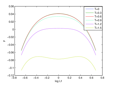
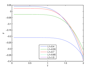
Figure 1. The graph on the left shows the free energy $F_{D}(L_{1},L_{2})$ as a function of $L_{1}$ when $V=L_{1}L_{2}=1$, at $T=0,0.3,0.6,0.9,1.2,1.5$. The graph on the right shows the free energy $F_{D}(L_{1},L_{2})$ as a function of $T$ when $L_{1}=0.4,0.55,0.7,0.85,1.0$ and $V=L_{1}L_{2}=1$.

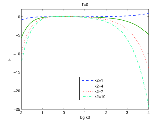
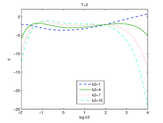
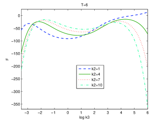
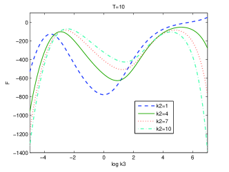
Figure 2. The free energy $F_{D}(L_{1},L_{2},L_{3})$ as a function of $k_{3}=L_{3}/L_{1}$ when $k_{2}=L_{2}/L_{1}=1,4,7,10$ and $V=L_{1}L_{2}L_{3}=1$, at $T=0,3,6,10$ respectively.

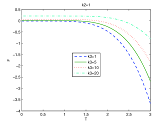
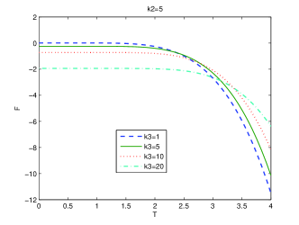
Figure 3. The free energy $F_{D}(L_{1},L_{2},L_{3})$ as a function of $T$ when $V=L_{1}L_{2}L_{3}=1$ and $k_{2}=L_{2}/L_{1}=1,5$ at $k_{3}=L_{3}/L_{1}=1,5,10,20$ respectively.

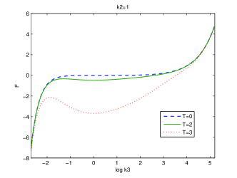
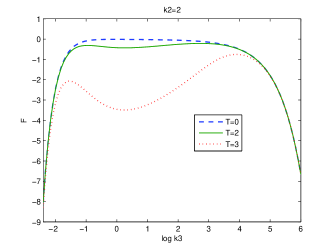
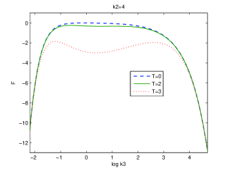
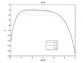
Figure 4. The free energy $F_{D}(L_{1},L_{2},L_{3})$ as a function of $k_{3}=L_{3}/L_{1}$ when $T=0,2,3$ and $V=L_{1}L_{2}L_{3}=1$ at $k_{2}=L_{2}/L_{1}=1,2,4,8$.

The low and high temperature expansions of the Casimir free energy $F_{D/N}$ can be obtained directly from (4.13) and the corresponding expansion for $F_{P}$. As in the periodic case, the zero temperature free energy for the Neumann case is always negative. However, the sign of the zero temperature free energy of the Dirichlet case depends on the parameters $L_{1},\ldots,L_{d}$. There have been a lots of discussions about this in the literature, see e.g. [15, 17, 18, 23]. By Remark 2.1, we know that fixing $L_{1},\ldots,L_{d}$, if $F^{0}_{D}$ is positive, then there exists a unique $T=T(L_{1},\ldots,L_{d})$ such that $F_{D}(L_{1},\ldots,L_{D})$ change from negative to positive. The scaling property of free energy (4.2) shows that $T(\lambda L_{1},\ldots,\lambda L_{d})=\lambda^{-1}T(L_{1},\ldots,L_{d})$. We study this transition temperature graphically for $d=2$ and $d=3$ (see Figure 5, 6).

Table 1
$k_{2}=L_{2}/L_{1}$ The range of $k_{3}=L_{3}/L_{1}$ where $F_{D}^{0}(L_{1},L_{2},L_{3})\geq 0$ 0.75 $k_{3}\geq 4.4972$ 1.0 $k_{3}\geq 4.2471$ 1.25 $k_{3}\geq 5.2999$ 1.5 $k_{3}\geq 8.8571$

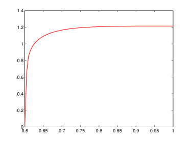
Figure 5. The transition temperature $T(L_{1},L_{2})$ for $F_{D}(L_{1},L_{2})$ as a function of $L_{1}$ when $V=L_{1}L_{2}=1$. $F_{D}^{0}(L_{1},L_{2})$ is positive when $0.6045^{2}\leq L_{1}/L_{2}\leq 1/0.6045^{2}$.

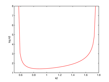
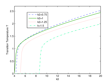
Figure 6. Left: When $0.5733\leq k_{2}=L_{2}/L_{1}\leq 1.7444$, there is a unique $\hat{k}_{3}=\hat{k}_{3}(k_{2})$ such that $F_{D}(L_{1},L_{2},L_{3})\geq 0$ for all $L_{3}/L_{1}\geq\hat{k}_{3}$. The graph shows $\log\hat{k}_{3}$ as a function of $k_{2}$. Right: The transition temperature $T(L_{1},L_{2},L_{3})$ for $F_{D}(L_{1},L_{2},L_{3})$ as a function of $k_{3}=L_{3}/L_{1}$ when $V=1$ and $k_{2}=L_{2}/L_{1}=0.75,1,1.25,1.5$.

In the high temperature regime, the leading term is

$$-\frac{L_{1}\ldots L_{d}}{\pi^{\frac{d+1}{2}}\beta^{d+1}}\Gamma\left(\frac{d+1}{2}\right)\zeta_{R}(d+1).$$

It comes from the $j=d$ term in (4.13) and it is again the Stefan-Boltzman term as in the periodic case (4.11). The term proportional to $\frac{1}{\beta}\log\beta$ is also present but in the Dirichlet case, its sign depends on $d$. Unlike the periodic boundary case (4.10), now we have terms proportional to $1/\beta^{j}$ for all $1\leq j\leq d+1$.

5. Massless vector field (electromagnetic field)

As discussed in [17], for massless vector (spin 1) field (or electromagnetic field) inside a $d$-dimensional space $\Omega$, the field strength is represented by a totally anti-symmetric rank-2 tensor $F^{\mu\nu}$ satisfying the equations

$$\partial_{\mu}\tilde{F}^{\mu\nu_{1}\ldots\nu_{d-2}}= 0,$$

$$\partial_{\mu}F^{\mu\nu}= j^{\nu},$$

where $\tilde{F}^{\mu_{1}\ldots\mu_{d-1}}=\varepsilon^{\mu_{1},\ldots,\mu_{d-1},\nu,\lambda}F_{\nu\lambda}$ is the dual tensor of $F^{\mu\nu}$ and $j^{\mu}$ is the current. In the vacuum state, $j^{\mu}=0$.

C.1. Perfectly Conducting Walls.   In the case that $\Omega=[0,L_{1}]\times\ldots\times[0,L_{d}]$ is a rectangular cavity with walls of infinite conductivity, the field satisfies the boundary condition

$$\left.n_{\mu}\tilde{F}^{\mu\nu_{1}\ldots\nu_{d-1}}\right|_{\partial\Omega}=0,$$

where $n_{\mu}$ is the unit vector normal to the walls $\partial\Omega$ and $n_{0}=0$. Introducing the potentials $A^{\mu}$ so that

$$F^{\mu\nu}=\partial^{\mu}A^{\nu}-\partial^{\nu}A^{\mu},\hskip 28.45274pt\partial^{0}=\partial_{0},\partial^{i}=-\partial_{i},\;\;1\leq i\leq d$$

and working in the radiation gauge with gauge condition

(5.1) $$A^{0}= 0,$$

$$\partial_{i}A^{i}= 0,$$

we find that the modes of the potentials are given by

$$A_{\mathbf{k}}^{i}= \alpha_{i}\cos\left(\frac{\pi k_{i}}{L_{i}}x_{i}\right)\prod_{\begin{subarray}{c}j=1\\ j\neq i\end{subarray}}^{d}\sin\left(\frac{\pi k_{j}}{L_{j}}x_{j}\right)e^{-i\omega_{\mathbf{k}}t},\hskip 28.45274pt1\leq i\leq d,$$

$$\text{where}\hskip 28.45274pt\mathbf{k}\in(\mathbb{N}\cup\{0\})^{d},\hskip 28.45274pt\omega_{\mathbf{k}}=\sqrt{\sum_{j=1}^{d}\left(\frac{\pi k_{j}}{L_{j}}\right)^{2}}.$$

The gauge condition (5.1) implies

(5.2) $$\sum_{i=1}^{d}\frac{\alpha_{i}k_{i}}{L_{i}}=0.$$

It is easy to see that if two of the $k_{i}$’s are zero, $\mathbf{A}_{\mathbf{k}}=(A_{\mathbf{k}}^{0},\ldots,A_{\mathbf{k}}^{d})$ is identically 0. On the other hand, if only a single $k_{i}$ is zero, then for $j\neq i$, $A_{\mathbf{k}}^{j}=0$ and (5.2) is trivially satisfied. When all $k_{i}$’s are nonzero, (5.2) implies that there is a $(d-1)$ degree of freedom for the vector $\vec{\alpha}=(\alpha_{1},\ldots,\alpha_{d})$ for any fixed $\mathbf{k}\in\mathbb{N}^{d}$. Therefore the zeta function for electromagnetic field confined in rectangular cavities with perfectly conducting walls is related to the zeta function for massless scalar field under Dirichlet boundary condition by

$$\zeta_{A_{C},d}(s;L_{1},\ldots,L_{d})= (d-1)\zeta_{D,d}(s;L_{1},\ldots,L_{d})$$

$$+\sum_{j=1}^{d}\zeta_{D,d-1}(s;L_{1},\ldots,L_{j-1},L_{j+1},\ldots,L_{d}).$$

There is no $\omega_{\mathbf{k}}=0$ mode and $\zeta_{A_{C},d}(0;L_{1},\ldots,L_{d})=0$. The corresponding free energy is

(5.3) $$F_{A_{C}}(L_{1},\ldots,L_{d})=(d-1)F_{D}(L_{1},\ldots,L_{d})+\sum_{j=1}^{d}F_{D}(L_{1},\ldots,L_{j-1},L_{j+1},\ldots,L_{d})$$

$$=2^{-d}\sum_{j=1}^{d}(-1)^{d-j}(2j-d-1)\sum_{1\leq m_{1}<\ldots<m_{j}\leq d}F_{p}(2L_{m_{1}},\ldots,2L_{m_{j}}).$$

C.2. Infinitely Permeable Walls.  In the case that $\Omega=[0,L_{1}]\times\ldots\times[0,L_{d}]$ is a rectangular cavity where the walls are infinitely permeable, the field satisfies the boundary condition

$$\left.n_{\mu}F^{\mu\nu}\right|_{\partial\Omega}=0.$$

Working in the radiation gauge (5.1), the modes of the potentials are given by

$$A_{\mathbf{k}}^{i}= \gamma_{i}\sin\left(\frac{\pi k_{i}}{L_{i}}x_{i}\right)\prod_{\begin{subarray}{c}j=1\\ j\neq i\end{subarray}}^{d}\cos\left(\frac{\pi k_{j}}{L_{j}}x_{j}\right)e^{-i\omega_{\mathbf{k}}t},\hskip 28.45274pt1\leq i\leq d,$$

$$\text{where}\hskip 56.9055pt\mathbf{k}\in(\mathbb{N}\cup\{0\})^{d},\hskip 28.45274pt\omega_{\mathbf{k}}=\sqrt{\sum_{j=1}^{d}\left(\frac{\pi k_{j}}{L_{j}}\right)^{2}}.$$

The gauge condition (5.1) implies

(5.4) $$\sum_{i=1}^{d}\frac{\gamma_{i}k_{i}}{L_{i}}=0.$$

If all the $k_{i}$’s are zero, $\mathbf{A}_{\mathbf{k}}=(A_{\mathbf{k}}^{0},\ldots,A_{\mathbf{k}}^{d})$ is identically 0. On the other hand, for $1\leq j\leq d$, fixing $1\leq r_{1}<\ldots<r_{d-j}\leq d$, let $1\leq m_{1}<\ldots<m_{j}\leq d$ be such that $\{m_{1},\ldots,m_{j},r_{1},\ldots,r_{d-j}\}=\{1,2,\ldots,d\}$. If $k_{r_{1}}=\ldots k_{r_{d-j}}=0$ and $k_{m_{1}}\neq 0,\ldots,k_{m_{j}}\neq 0$, then $A_{\mathbf{k}}^{r_{l}}=0$ for $1\leq l\leq d-j$ and (5.4) reduces to $\sum_{l=1}^{j}\frac{\gamma_{m_{l}}k_{m_{l}}}{L_{m_{l}}}=0$. This implies that there is a $(j-1)$ degrees of freedom for the vector $(\gamma_{m_{1}},\ldots,\gamma_{m_{j}})$ for any fixed $(k_{m_{1}},\ldots,k_{m_{j}})\in\mathbb{N}^{j}$. Therefore the zeta function for electromagnetic field confined in a closed rectangular cavity with infinitely permeable walls is related to the zeta function for massless scalar field under Dirichlet boundary condition by

$$\zeta_{A_{B},d}(s;L_{1},\ldots,L_{d})= \sum_{j=2}^{d}(j-1)\sum_{1\leq m_{1}<\ldots<m_{j}\leq d}\zeta_{D,j}\left(s;L_{m_{1}},\ldots,L_{m_{j}}\right).$$

There is no $\omega_{\mathbf{k}}=0$ mode and $\zeta_{A_{B},d}(0;L_{1},\ldots,L_{d})=0$. The corresponding free energy is (see the detail computation in the appendix):

(5.5) $$F_{A_{B}}(L_{1},\ldots,L_{d})= \sum_{j=2}^{d}(j-1)\sum_{1\leq m_{1}<\ldots<m_{j}\leq d}F_{D}\left(s;L_{m_{1}},\ldots,L_{m_{j}}\right).$$

$$= 2^{-d}\sum_{j=1}^{d}(2j-d-1)\sum_{1\leq m_{1}<\ldots<m_{j}\leq d}F_{p}(2L_{m_{1}},\ldots,2L_{m_{j}}).$$

Notice that when $d=2$, $F_{A_{C}}(L_{1},L_{2})=F_{N}(L_{1},L_{2})$, $F_{A_{B}}(L_{1},L_{2})=F_{D}(L_{1},L_{2})$ and when $d=3$, $F_{A_{C}}(L_{1},L_{2},L_{3})=F_{A_{B}}(L_{1},L_{2},L_{3})$.

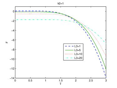
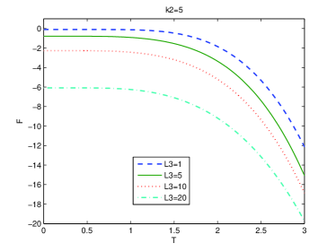
Figure 7. The free energy $F_{A_{C}}(L_{1},L_{2},L_{3})$ as a function of $T$ when $V=L_{1}L_{2}L_{3}=1$ and $k_{2}=L_{2}/L_{1}=1,5$ at $k_{3}=L_{3}/L_{1}=1,5,10,20$ respectively.

Under the simultaneous space–time scaling $\beta\mapsto\lambda\beta$, $L_{i}\mapsto\lambda L_{i},1\leq i\leq d$, both $F_{A_{C}}(L_{1},\ldots,L_{d})$ and $F_{A_{B}}(L_{1},\ldots,L_{d})$ transform as

$$F_{A_{C/B}}(L_{1},\ldots,L_{d})\mapsto\lambda^{-1}F_{A_{C/B}}(L_{1},\ldots,L_{d}),$$

and thus the thermodynamic relation (4.9) holds.

The low and high temperature expansions of the free energy $F_{A_{C/B}}$ can be obtained from the corresponding expansion of $F_{P}$ using (5.3) and (5.5). The sign of the zero temperature energy $F_{A_{C/B}}^{0}(L_{1},\ldots,L_{d})$ also depends on the relative size of $L_{1},\ldots,L_{d}$.

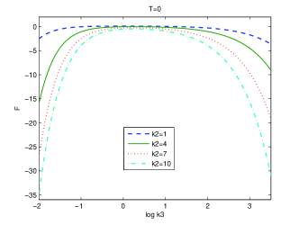
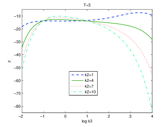
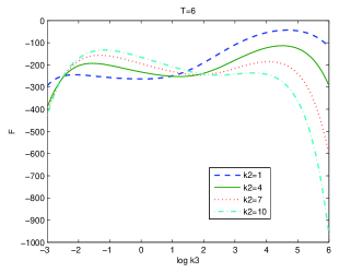
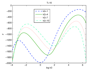
Figure 8. The free energy $F_{A_{C}}(L_{1},L_{2},L_{3})$ as a function of $k_{3}=L_{3}/L_{1}$ when $k_{2}=L_{2}/L_{1}=1,4,7,10$ and $V=L_{1}L_{2}L_{3}=1$, at $T=0,3,6,10$ respectively.

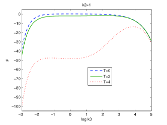
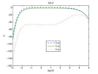
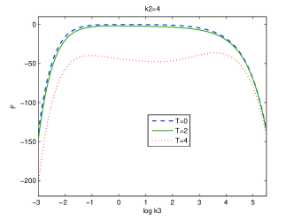
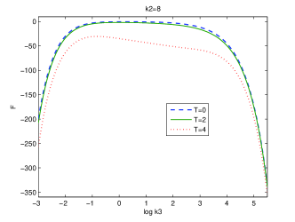
Figure 9. The free energy $F_{A_{C}}(L_{1},L_{2},L_{3})$ as a function of $k_{3}=L_{3}/L_{1}$ when $T=0,2,4$ and $V=L_{1}L_{2}L_{3}=1$ at $k_{2}=L_{2}/L_{1}=1,2,4,8$.

Table 2
$k_{2}=L_{2}/L_{1}$ The range of $k_{3}=L_{3}/L_{1}$ where $F_{A_{C}}^{0}(L_{1},L_{2},L_{3})\geq 0$ 0.75 $0.3555\leq k_{3}\leq 2.7033$ 1. $0.4083\leq k_{3}\leq 3.4298$ 1.25 $0.4580\leq k_{3}\leq 3.6219$ 1.5 $0.5057\leq k_{3}\leq 3.4957$

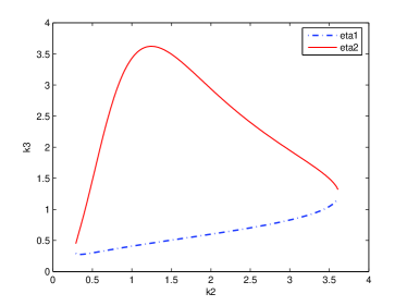
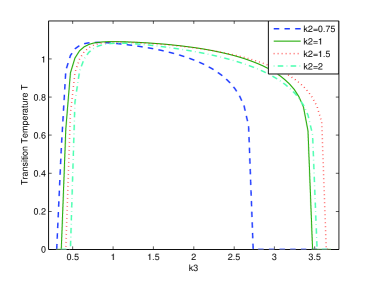
Figure 10. Left: When $0.2761\leq k_{2}=L_{2}/L_{1}\leq 3.6195$, there exist $\eta_{1}(k_{2})$ and $\eta_{2}(k_{2})$ such that $F_{A_{C}}(L_{1},L_{2},L_{3})\geq 0$ for all $\eta_{1}(k_{2})\leq L_{3}/L_{1}\leq\eta_{2}(k_{2})$. The graph shows $\eta_{1}$ and $\eta_{2}$ as functions of $k_{2}$. Right: The transition temperature $T(L_{1},L_{2},L_{3})$ for $F_{A_{C}}(L_{1},L_{2},L_{3})$ as a function of $k_{3}=L_{3}/L_{1}$ when $V=1$ and $k_{2}=1,1.5,2$.

In the high temperature regime, the leading term is

$$-(d-1)\frac{L_{1}\ldots L_{d}}{\pi^{\frac{d+1}{2}}\beta^{d+1}}\Gamma\left(\frac{d+1}{2}\right)\zeta_{R}(d+1),$$

which is $(d-1)$ times the leading term in the scalar field case. This is due to the fact that electromagnetic field in $d+1$ dimensional space–time has $d-1$ polarization states. The term proportional to $\frac{1}{\beta}\log\beta$ still present. When $d$ is even, there are terms proportional to $\frac{1}{\beta^{j}}$ for all $1\leq j\leq d+1$. When $d$ is odd, there are terms proportional to $\frac{1}{\beta^{j}}$ for all $1\leq j\leq d+1$ except for $j=\frac{d+3}{2}$.

When $d=3$, we find that the zero point energy $F_{A_{C}}^{0}(L_{1},L_{2},L_{3})$ is given by

$$F_{A_{C}}^{0}(L_{1},L_{2},L_{3})=F_{A_{B}}^{0}(L_{1},L_{2},L_{3})$$

$$= -\frac{L_{1}L_{2}L_{3}}{16\pi^{2}}\sum_{\mathbf{k}\in{\mathbb{Z}}^{3}\setminus\{\mathbf{0}\}}\frac{1}{\left((L_{1}k_{1})^{2}+(L_{2}k_{2})^{2}+(L_{3}k^{3})^{2}\right)^{2}}+\frac{\pi}{48}\left(\frac{1}{L_{1}}+\frac{1}{L_{2}}+\frac{1}{L_{3}}\right),$$

which is a well known result (see e.g., [23]). We show graphically some particular values of the transition temperature $T(L_{1},L_{2},L_{d})$ for $F_{A_{C}}(L_{1},L_{2},L_{3})$ in Figure 10.

On the other hand, the high temperature expansion of $F_{A_{C}}(L_{1},L_{2},L_{3})=F_{A_{B}}(L_{1},L_{2},L_{3})$ is

(5.6) $$F_{A_{C}}(L_{1},L_{2},L_{3})=F_{A_{B}}(L_{1},L_{2},L_{3})=-\frac{\pi^{2}}{45}\frac{L_{1}L_{2}L_{3}}{\beta^{4}}+\frac{\pi}{12}\frac{L_{1}+L_{2}+L_{3}}{\beta^{2}}$$

$$+\frac{1}{2\beta}\log\beta-\frac{1}{8\beta}Z_{E,3}^{\prime}\left(0;L_{1}^{-1},L_{2}^{-1},L_{3}^{-1}\right)-\frac{1}{4\beta}\log(8\pi L_{1}L_{2}L_{3})$$

$$-\frac{L_{1}L_{2}L_{3}}{2\beta^{2}}\sum_{\mathbf{k}\in{\mathbb{Z}}^{3}\setminus\{\mathbf{0}\}}\frac{1}{\sum_{j=1}^{3}[L_{j}k_{j}]^{2}}\frac{e^{\frac{4\pi}{\beta}\sqrt{\sum_{j=1}^{3}[L_{j}k_{j}]^{2}}}}{\left(e^{\frac{4\pi}{\beta}\sqrt{\sum_{j=1}^{3}[L_{j}k_{j}]^{2}}}-1\right)^{2}}$$

$$-\frac{L_{1}L_{2}L_{3}}{8\pi\beta}\sum_{\mathbf{k}\in{\mathbb{Z}}^{3}\setminus\{\mathbf{0}\}}\frac{1}{\left[\sum_{j=1}^{3}[L_{j}k_{j}]^{2}\right]^{3/2}}\frac{1}{e^{\frac{4\pi}{\beta}\sqrt{\sum_{j=1}^{3}[L_{j}k_{j}]^{2}}}-1}$$

$$+\frac{1}{2\beta}\sum_{k=1}^{\infty}\frac{1}{k}\left[\frac{1}{e^{\frac{4\pi kL_{1}}{\beta}}-1}+\frac{1}{e^{\frac{4\pi kL_{2}}{\beta}}-1}+\frac{1}{e^{\frac{4\pi kL_{3}}{\beta}}-1}\right].$$

Our result gives the correct high temperature limit stipulated by Ambjørn and Wolfram [17] (equation (7.12)). However, they only obtained the first three terms. To the best of our knowledge, we are not aware of any existing study that calculate the high temperature limit to the degree of accuracy obtained here. We would like to emphasize that the formula (5.6) is valid for all temperature. In [29], the authors calculate this free energy by a different method. They gave the same first two leading terms as above, and no explicit formulas for the remaining terms are given.

6. From closed cavity to general case

There exist many papers on the Casimir energy of massless scalar field or Casimir energy of electromagnetic field confined in a $p$-dimensional rectangular cavity in a $d$-dimensional space [17, 14, 15, 18, 19, 20, 22, 24, 25, 26, 27, 33]. A $p$-dimensional rectangular cavity in a $d$-dimensional space is a space of the form $\Omega_{p,d}=[0,L_{1}]\times\ldots\times[0,L_{p}]\times\mathbb{R}^{d-p}$, where $0\leq p\leq d$. It can be considered as the limiting case of the closed cavity where $L_{1},\ldots,L_{p}\ll L_{p+1}=\ldots=L_{d}=L$ or $L_{j}\rightarrow\infty$ for $p+1\leq j\leq d$. In the existing literature, when calculating the Casimir free energy, usually after setting up the zeta function over $(k_{1},\ldots,k_{d})$ in a suitable set, the summation over $k_{p+1},\ldots,k_{d}$ is changed to integration. From the mathematical point of view, this is not a rigorous treatment since the summation expression for the zeta function only works for $\text{Re}\;s>\frac{d}{2}$, which does not include the point $s=0$. To justify this procedure, one actually need to justify that the processes of taking analytic continuation and taking limit $L_{j}\rightarrow\infty$ for $p+1\leq j\leq d$ can be interchanged. In this section, we will directly take the limit $L_{j}\rightarrow\infty$ for $p+1\leq j\leq d$ in the expression of Casimir energy for fields inside a closed rectangular cavity to obtain the energy of the fields inside a non-closed rectangular cavity. To be more precise, the limit when $L_{j}\rightarrow\infty$ for $p+1\leq j\leq d$ of the free energy $F(L_{1},\ldots,L_{d})$ is always infinite. Therefore we shall consider the free energy density $f$ defined as the limit

$$f_{d}(L_{1},\ldots,L_{p})=\lim_{\begin{subarray}{c}L_{i}\rightarrow\infty\\ p+1\leq i\leq d\end{subarray}}\frac{F(L_{1},\ldots,L_{d})}{L_{p+1}\ldots L_{d}}.$$

In the following, we assume that $0\leq p\leq d-1$. By putting $m=d-p$, $a_{j}=2\pi/L_{p+j},1\leq j\leq d-p$, $a_{d-p+1}=2\pi/\beta$ and $a_{j}=2\pi/L_{j-d+p-1},d-p+2\leq j\leq d+1$ in (3.6), we find that the free energy $F_{P}(L_{1},\ldots,L_{d})$ (4.1) is equal to

$$F_{P}(L_{1},\ldots,L_{d})= -\frac{1}{2\beta}Z_{E,d-p}^{\prime}\left(0;\frac{2\pi}{L_{p+1}},\ldots,\frac{2\pi}{L_{d}}\right)-\frac{1}{\beta}\log\beta$$

$$-\frac{\pi^{-\frac{d+1}{2}}\Gamma\left(\frac{d+1}{2}\right)}{2(2\pi)^{d+1}}L_{1}\ldots L_{d}Z_{E,p+1}\left(\frac{d+1}{2};\frac{\beta}{2\pi},\frac{L_{1}}{2\pi},\ldots,\frac{L_{p}}{2\pi}\right)$$

$$-\frac{1}{2\beta}R_{n,d-p}\left(\frac{2\pi}{\beta},\frac{2\pi}{L_{1}},\ldots,\frac{2\pi}{L_{d}}\right),$$

where $R_{n,m}(a_{1},\ldots,a_{n})$ is defined by (3.7). Now the last term goes to zero as $L_{j}\rightarrow\infty$ for $p+1\leq j\leq d$ (see appendix). Therefore,

(6.1) $$f_{P,d}(L_{1},\ldots,L_{p})= -\frac{1}{2\beta}\lim_{\begin{subarray}{c}L_{i}\rightarrow\infty\\ p+1\leq i\leq d\end{subarray}}\frac{1}{L_{p+1}\ldots,L_{d}}Z_{E,d-p}^{\prime}\left(0;\frac{2\pi}{L_{p+1}},\ldots,\frac{2\pi}{L_{d}}\right)$$

$$-\frac{\pi^{-\frac{d+1}{2}}\Gamma\left(\frac{d+1}{2}\right)}{2(2\pi)^{d+1}}L_{1}\ldots L_{p}Z_{E,p+1}\left(\frac{d+1}{2};\frac{\beta}{2\pi},\frac{L_{1}}{2\pi},\ldots,\frac{L_{p}}{2\pi}\right).$$

Next we want to show that the first term in (6.1) is also zero, i.e. we need to show that

$$\lim_{\begin{subarray}{c}a_{i}\rightarrow 0\\ 1\leq i\leq n\end{subarray}}a_{1}\ldots a_{n}Z_{E,n}^{\prime}\left(0;a_{1},\ldots,a_{n}\right)=0.$$

When $n=1$, we have

$$Z_{E,1}^{\prime}(0;a)=2\log\frac{a}{2\pi},$$

therefore $\lim_{a\rightarrow 0}\left[aZ_{E,1}^{\prime}(0;a)\right]=0$. When $n>1$, equation (3.6) gives

$$Z_{E,n}^{\prime}\left(0;a_{1},\ldots,a_{n}\right)$$

$$= Z_{E,n-1}^{\prime}\left(0;a_{1},\ldots,a_{n-1}\right)+\frac{2\pi^{-n/2}a_{n}^{n-1}\Gamma\left(\frac{n}{2}\right)}{\left[\prod_{j=1}^{n-1}a_{j}\right]}\zeta_{R}(n)+R_{n,n-1}(a_{1},\ldots,a_{n}).$$

Using a similar argument as before (see appendix),

$$\lim_{\begin{subarray}{c}a_{i}\rightarrow 0\\ 1\leq i\leq n-1\end{subarray}}a_{1}\ldots a_{n-1}R_{n,n-1}(a_{1},\ldots,a_{n})=0.$$

On the other hand, it is obvious that

$$\lim_{\begin{subarray}{c}a_{i}\rightarrow 0\\ 1\leq i\leq n-1\end{subarray}}a_{1}\ldots a_{n}\frac{2\pi^{-n/2}a_{n}^{n-1}\Gamma\left(\frac{n}{2}\right)}{\left[\prod_{j=1}^{n-1}a_{j}\right]}\zeta_{R}(n)=0.$$

Therefore,

$$\lim_{\begin{subarray}{c}a_{i}\rightarrow 0\\ 1\leq i\leq n\end{subarray}}a_{1}\ldots a_{n}Z_{E,n}^{\prime}\left(0;a_{1},\ldots,a_{n}\right)=\lim_{\begin{subarray}{c}a_{i}\rightarrow 0\\ 1\leq i\leq n\end{subarray}}a_{1}\ldots a_{n}Z_{E,{n-1}}^{\prime}\left(0;a_{1},\ldots,a_{n-1}\right),$$

and we obtain by induction on $n$ that this is zero. Consequently, we find from (6.1) that

(6.2) $$f_{P,d}(L_{1},\ldots,L_{p})=-\frac{\Gamma\left(\frac{d+1}{2}\right)}{2\pi^{\frac{d+1}{2}}}L_{1}\ldots L_{p}Z_{E,p+1}\left(\frac{d+1}{2};\beta,L_{1},\ldots,L_{p}\right)$$

and this agrees with the result in [17] obtained by dimensional regularization method. Notice that the right hand side of (6.2) is not defined when $p=d$. Under the simultaneous space–time scaling $\beta\rightarrow\lambda\beta$, $L_{i}\mapsto\lambda L_{i},1\leq i\leq d$, the free energy density $f_{P,d}(L_{1},\ldots,L_{p})$ transforms as

(6.3) $$f_{P,d}(L_{1},\ldots,L_{p})\mapsto\lambda^{p-d-1}f_{P,d}(L_{1},\ldots,L_{p}).$$

Now using the fact that

$$\lim_{\begin{subarray}{c}L_{j}\rightarrow\infty\\ p+1\leq j\leq d\end{subarray}}\frac{F_{P}\left(2L_{m_{1}},\ldots,2L_{m_{j}},2L_{p+1},\ldots,2L_{d}\right)}{L_{p+1}\ldots L_{d}}$$

$$= 2^{d-p}\lim_{\begin{subarray}{c}L_{j}\rightarrow\infty\\ p+1\leq j\leq d\end{subarray}}\frac{F_{P}\left(2L_{m_{1}},\ldots,2L_{m_{j}},2L_{p+1},\ldots,2L_{d}\right)}{(2L_{p+1})\ldots(2L_{d})}=2^{d-p}f_{P,d}\left(2L_{m_{1}},\ldots,2L_{m_{j}}\right),$$

and (4.13), (5.3), we find that the free energy densities $f_{D,d}(L_{1},\ldots,L_{p})$, $f_{N,d}(L_{1},\ldots,L_{p})$, $f_{A_{C},d}(L_{1},\ldots,L_{p})$, $f_{A_{B},d}(L_{1},\ldots,L_{p})$ for massless scalar field under Dirichlet and Neumann boundary conditions and for electromagnetic field confined in cavity with perfectly conducting walls and with infinitely permeable walls are related to the free energy for massless scalar field under periodic condition by:

(6.4) $$f_{D/N,d}(L_{1},\ldots,L_{p})=2^{-p}\sum_{j=0}^{p}(\mp 1)^{p-j}\sum_{1\leq m_{1}<\ldots<m_{j}\leq p}f_{P,j+d-p}(2L_{m_{1}},\ldots,2L_{m_{j}})$$

$$f_{A_{C/B,d}}(L_{1},\ldots,L_{p})$$

$$= 2^{-p}\sum_{j=0}^{p}(\mp 1)^{p-j}(d-1-2p+2j)\sum_{1\leq m_{1}<\ldots<m_{j}\leq p}f_{P,j+d-p}(2L_{m_{1}},\ldots,2L_{m_{j}}).$$

The scaling behavior of the free energy density in these cases is the same as the periodic case (6.3).

When $p=0$, we obtain the vacuum energy of free massless scalar field and electromagnetic field in $\mathbb{R}^{d}$:

(6.5) $$f_{P,d}=f_{D,d} =f_{N,d}=-\frac{\Gamma\left(\frac{d+1}{2}\right)}{\pi^{\frac{d+1}{2}}}\frac{1}{\beta^{d+1}}\zeta_{R}(d+1),$$

$$f_{A_{C/B,d}}= -(d-1)\frac{\Gamma\left(\frac{d+1}{2}\right)}{\pi^{\frac{d+1}{2}}}\frac{1}{\beta^{d+1}}\zeta_{R}(d+1),$$

which are the Stefan-Boltzmann terms. These equations are reasonable since when extending to the space $\mathbb{R}^{d}$, the boundary disappears and the vacuum energy should be the same no matter what boundary conditions we start with.

6.1. Low Temperature Expansion

When $1\leq p\leq d-1$, by putting $m=p$, $a_{i}=L_{i},1\leq i\leq p$, $a_{p+1}=\beta$ in the Chowla-Selberg formula (3.3), we obtain the low temperature ($T\ll 1$) expansion of the free energy density (6.2):

(6.6) $$f_{P,d}(L_{1},\ldots,L_{p})$$

$$= -\frac{\Gamma\left(\frac{d+1}{2}\right)}{2\pi^{\frac{d+1}{2}}}L_{1}\ldots L_{p}Z_{E,p}\left(\frac{d+1}{2};L_{1},\ldots,L_{p}\right)-\frac{\Gamma\left(\frac{d-p+1}{2}\right)}{\pi^{\frac{d-p+1}{2}}}\frac{\zeta_{R}(d-p+1)}{\beta^{d-p+1}}$$

$$-\frac{2}{\beta^{\frac{d-p+1}{2}}}\sum_{m=1}^{\infty}\sum_{\mathbf{k}\in{\mathbb{Z}}^{p}\setminus\{\mathbf{0}\}}\frac{1}{m^{\frac{d-p+1}{2}}}\left(\sum_{j=1}^{p}\left[\frac{k_{j}}{L_{j}}\right]^{2}\right)^{\frac{d+1-p}{4}}K_{\frac{d-p+1}{2}}\left(2\pi m\beta\sqrt{\sum_{j=1}^{p}\left[\frac{k_{j}}{L_{j}}\right]^{2}}\right).$$

The first term gives the zero temperature energy density and the sum of the last two terms is the thermal correction. Note that now the thermal correction contains a term proportional to $\beta^{-\frac{d-p+1}{2}}$. As usual the last term decays exponentially. We show in the appendix that the sum of the thermal correction is equal to

$$\frac{1}{(2\pi)^{d-p}\beta}\int_{\mathbb{R}^{d-p}}\sum_{\mathbf{k}\in{\mathbb{Z}}^{p}}\log\left(1-e^{-\beta\sqrt{\sum_{j=1}^{p}\left[\frac{2\pi k_{j}}{L_{j}}\right]^{2}+|\mathbf{w}|^{2}}}\right)dw_{1}\ldots dw_{d-p},$$

in agreement with the usual integration prescription to obtain the limit $L_{j}\rightarrow\infty$ for $p+1\leq j\leq d$. From this formula, we can verify as in the closed cavity case that the free energy density is a decreasing function of temperature. On the other hand, (6.2) implies that the Casimir free energy is negative at all temperature for all $p$ and $d$ such that $0\leq p<d$.

Compare to (4.5), we find that we cannot simply set $p=d$ in (6.6) to obtain the free energy in the closed cavity case (4.5) due to the second term. In fact, by using physics argument, Ambjørn and Wolfram [17] has argued that in order to obtain the free energy for closed cavity from this formula, it is necessary to omit the second term.

Using (6.4) and (6.6), one can also obtain the low temperature expansion of the free energy densities $f_{D/N,d}$ and $f_{A_{C/B,d}}$ for $1\leq p\leq d-1$. We find that in the case of scalar field with Dirichlet boundary condition, the thermal correction is an exponentially decay term, whereas for the scalar field with Neumann boundary condition and also for electromagnetic field confined in a cavity with infinitely permeable walls, there is an extra term proportional to $\beta^{-\frac{d-p+1}{2}}$ and for the electromagnetic field confined in a cavity with perfectly conducting walls, this extra term only present when $p=1$. Just like the periodic case, we can show that the thermal corrections are equal to

(6.7) $$\frac{1}{(2\pi)^{d-p}\beta}\int_{\mathbb{R}^{d-p}}\sum_{\mathbf{k}\in(\mathbb{N}\cup\{0\})^{p}}M_{\mathcal{BC}}(\mathbf{k})\log\left(1-e^{-\beta\sqrt{\sum_{j=1}^{p}\left[\frac{\pi k_{j}}{L_{j}}\right]^{2}+|\mathbf{w}|^{2}}}\right)dw_{1}\ldots dw_{d-p},$$

which is in agreement with the usual integration prescription. Here $\mathcal{BC}=D,N,A_{C},A_{B}$ and

$$M_{D}(\mathbf{k})= \begin{cases}1,\hskip 28.45274pt&\text{if}\;\;\mathbf{k}\in\mathbb{N}^{p},\\ 0,&\text{otherwise},\end{cases}$$

$$M_{N}(\mathbf{k})= \;1\hskip 28.45274pt\forall\mathbf{k}\in(\mathbb{N}\cup\{0\})^{p},$$

$$M_{A_{C}}(\mathbf{k})= \begin{cases}d-1,\hskip 28.45274pt&\text{if}\;\;k_{i}\neq 0\;\text{for all}\;1\leq i\leq p,\\ 1,&\text{if}\;\;k_{i}=0\;\text{for some $i$, and $k_{j}\neq 0$ for all other $j\neq i$},\\ 0,&\text{otherwise}.\end{cases}$$

$$M_{A_{B}}(\mathbf{k})= \;d-p+j-1,\hskip 28.45274pt\text{if exactly $j$ of the $k_{1},\ldots,k_{p}$ are nonzero.}$$

From this, we can also conclude that the free energy density is a decreasing function of temperature. In the case of scalar field with Neumann condition, we can even generalize the conclusion to that the Casimir energy is always negative. However, in the case of scalar field with Dirichlet condition and the cases of electromagnetic fields, the sign of the Casimir free energy depends on $p,d,T$ and the values of $L_{1},\ldots,L_{p}$. There have been some discussions on this point in [15, 18, 24, 33].

6.2. High Temperature Expansion

When $1\leq p\leq d-1$, by putting $m=1$, $a_{1}=\beta$, $a_{i}=L_{i-1},2\leq i\leq p+1$, in the Chowla-Selberg formula (3.3), we obtain the high temperature ($T\gg 1$) expansion of the free energy density (6.2):

(6.8) $$f_{P,d}(L_{1},\ldots,L_{p})=-\frac{\Gamma\left(\frac{d+1}{2}\right)}{\pi^{\frac{d+1}{2}}}L_{1}\ldots L_{p}\frac{\zeta_{R}(d+1)}{\beta^{d+1}}$$

$$-\frac{\Gamma\left(\frac{d}{2}\right)}{2\pi^{\frac{d}{2}}}L_{1}\ldots L_{p}\frac{1}{\beta}Z_{E,p}\left(\frac{d}{2};L_{1},\ldots,L_{p}\right)$$

$$-\frac{2L_{1}\ldots L_{p}}{\beta^{\frac{d+2}{2}}}\sum_{\mathbf{k}\in{\mathbb{Z}}^{p}\setminus\{\mathbf{0}\}}\sum_{m=1}^{\infty}m^{\frac{d}{2}}\left(\sum_{j=1}^{p}\left[L_{j}k_{j}\right]^{2}\right)^{-\frac{d}{4}}K_{\frac{d}{2}}\left(\frac{2\pi m}{\beta}\sqrt{\sum_{j=1}^{p}\left[L_{j}k_{j}\right]^{2}}\right),$$

which agrees with the result obtained in [17]. The leading term is the Stefan-Boltzmann term which is equal to the vacuum energy of $\mathbb{R}^{d}$ (6.5). The second term is of order $\beta^{-1}$ and it is divergent for $p=d$. In [17], Ambjørn and Wolfram argued that to obtain the $p=d$ case from this formula, one needs to remove the divergence by subtracting the free Bose gas result, i.e. replace the second term by

$$-\frac{1}{2}\lim_{p\rightarrow d}\left(\frac{\Gamma\left(\frac{d}{2}\right)}{\pi^{\frac{d}{2}}}L_{1}\ldots L_{p}\frac{1}{\beta}Z_{E,p}\left(\frac{d}{2};L_{1},\ldots,L_{p}\right)-\frac{\Gamma\left(\frac{d-p+1}{2}\right)}{\pi^{\frac{d-p+1}{2}}}Z_{E,1}\left(\frac{d-p+1}{2};\beta\right)\right)$$

$$= -\frac{1}{2\beta}\left(Z_{E,p}^{\prime}\left(0;L_{1}^{-1},\ldots,L_{p}^{-1}\right)-Z_{E,1}^{\prime}(0,\beta^{-1})\right).$$

Comparing to (4.10), we have shown mathematically that this is indeed the case. Using (6.4) and (6.8), one can also obtain the high temperature expansion of the free energy densities $f_{D/N,d}$ and $f_{A_{C/B},d}$ for $1\leq p\leq d-1$. We find that the leading term for all the cases is equal to the vacuum energy of $\mathbb{R}^{d}$ (6.5). In the cases of Dirichlet and Neumann conditions, there are terms proportional to $\beta^{-j}$ for every $d-p+1\leq j\leq d+1$ as well as for $j=1$. For electromagnetic field, when $d$ is odd and $p\geq(d+1)/2$, there is no term proportional to $\beta^{-\frac{d+1}{2}}.$

7. Conclusion

We have provided a rigorous derivation of the Casimir free energy at finite temperature for massless scalar fields and electromagnetic field confined in a closed rectangular cavity with different boundary conditions by zeta regularization method. By applying Chowla-Selberg formula, we obtained explicit formulas for the low and high temperature expansions of the free energy, which can be written as a sum of polynomial order terms in $T$ or $T^{-1}$ plus an exponentially decay term. To the best of our knowledge, such explicit formulas for the low and high temperature expansions of the free energy of fields confined within closed cavities has not been obtained previously.

We noted that for all the cases considered, the free energy at finite temperature $F(\beta;L_{1},\ldots,L_{d})$ transforms as

$$F(\beta;L_{1},\ldots,L_{d})\mapsto F(\lambda\beta;\lambda L_{1},\ldots,\lambda L_{d})=\lambda^{-1}F(\beta;L_{1},\ldots,L_{d}),$$

under the simultaneous space–time scaling $\beta\mapsto\lambda\beta$, $L_{i}\mapsto\lambda L_{i},1\leq i\leq d$. This in turn implies the thermodynamic relation

$$F=(P_{1}+\ldots+P_{d})V-TS,$$

which has not been observed.

On the other hand, we also show that the free energy in all the cases considered is a decreasing function of temperature. For massless scalar field under periodic and Neumann boundary conditions, the free energy is negative for all temperature. For massless scalar field under Dirichlet boundary condition and for electromagnetic fields, the free energy might be positive at zero temperature. When this happens, there is a unique transition temperature at which the free energy change from positive to negative. This transition temperature is shown graphically for $d=2$ and $d=3$. We believe that for massless scalar field under Dirichlet boundary condition and for electromagnetic fields, when $d\geq 4$, the zero temperature free energy will also be positive for $(L_{1},\ldots,L_{d})$ lying in some domain of $\mathbb{R}^{d}$. A detail study of this is left to another paper.

In the last section, we show how the free energy for a non-closed rectangular cavity can be obtained by letting the size of some directions of a closed cavity going to infinity. We prove that the results are in agreement with that based on the integration prescription usually adopted by other authors.

We remark that the discussion given in this paper focused mainly on the low and high temperature expansions of the free energy and the properties of the free energy. We have not dealt with other thermodynamic quantities such as the force, pressure, internal energy and entropy. We hope to consider these quantities in a future work.

Finally, we would like to point out that there exist some controversies regarding imposing boundary conditions on a quantum field. Deutsch and Candelas [46] were the first to study the nonintegrable divergences in the renormalized energy density near boundaries. This problem has been re-examined by Baacke and Krüsemann [47] and analyzed in detail recently by Jaffe [48, 49] and Graham et al [50, 51, 52, 53]. These authors showed that the imposition of boundary conditions on quantum fields in Casimir effect calculations leads to non-renormalizable infinities. As a result, fixing boundary conditions ab initio invariably results in divergences which cannot be removed by renormalization. Basically this problem for electromagnetic field with Dirichlet boundary condition can be stated as that no real material is perfectly conducting at arbitrary high frequencies. In order to overcome this serious problem, Graham and collaborators have developed a new approach which replaces the boundary condition by a renormalizable coupling between the fluctuating field and a non-dynamical background field representing the material. On the other hand, there were responses from Milton [54], Fulling [55] and Elizalde [56] with various attempts to resolve this issue. Here we would like to mention the effort by Elizalde who has tried to explain the presence of infinities as a result of drastic reduction of eigenstates when boundary condition is imposed. He has proposed to complement the zeta function method with the Hadamard regularization in order to make sense of infinities present in the boundary value problems in Casimir energy calculations. However such an approach cannot be taken as a substitute of the more physical treatment given in ref. [48, 49, 50, 51, 52, 53]. The system considered in this paper can be regarded as ideal cases, for which zeta function technique is still a useful tool for regularization of vacuum energy density. For a more physical treatment, one has no choice but have to take into account of the problem of singular behavior near a boundary.

Acknowledgement  The authors would like to thank Malaysian Academy of Sciences, Ministry of Science, Technology and Innovation for funding this project under the Scientific Advancement Fund Allocation (SAGA) Ref. No P96c.

Appendix A

In this appendix, we gather some mathematical formulas and estimates that we need.

1. We want to prove (5.3). By equation (4.13), we find that

$$F_{A_{B}}\left(L_{1},\ldots,L_{d}\right)= \sum_{j=1}^{d}c_{j;d}\sum_{1\leq m_{1}<\ldots<m_{j}\leq d}F_{P}\left(L_{m_{1}},\ldots,L_{m_{j}}\right),$$

$$\text{where}\hskip 28.45274ptc_{j;d}=\sum_{k=j}^{d}(-1)^{k-j}(k-1)\begin{pmatrix}d-j\\ k-j\end{pmatrix}2^{-k}.$$

Now we compute $c_{j;d}$.

$$c_{j;d}= \sum_{k=0}^{d-j}(-1)^{k}(k+j-1)\begin{pmatrix}d-j\\ k\end{pmatrix}2^{-k-j}$$

$$= 2^{-j}\left(\sum_{k=0}^{d-j}(-1)^{k}k\begin{pmatrix}d-j\\ k\end{pmatrix}2^{-k}+(j-1)\sum_{k=0}^{d-j}(-1)^{k}\begin{pmatrix}d-j\\ k\end{pmatrix}2^{-k}\right)$$

$$= 2^{-j}\left((d-j)\sum_{k=1}^{d-j}(-1)^{k}\begin{pmatrix}d-j-1\\ k-1\end{pmatrix}2^{-k}+(j-1)\sum_{k=0}^{d-j}(-1)^{k}\begin{pmatrix}d-j\\ k\end{pmatrix}2^{-k}\right)$$

$$= 2^{-j}\left(-\frac{(d-j)}{2}\sum_{k=0}^{d-j-1}(-1)^{k}\begin{pmatrix}d-j-1\\ k\end{pmatrix}2^{-k}+(j-1)\sum_{k=0}^{d-j}(-1)^{k}\begin{pmatrix}d-j\\ k\end{pmatrix}2^{-k}\right)$$

$$= 2^{-j}\left(-\frac{(d-j)}{2}\left(1-\frac{1}{2}\right)^{d-j-1}+(j-1)\left(1-\frac{1}{2}\right)^{d-j}\right)$$

$$= 2^{-d}(2j-d-1).$$

2. We want to show that

$$\lim_{\begin{subarray}{c}a_{i}\rightarrow 0\\ 1\leq i\leq m\end{subarray}}\left[\prod_{j=1}^{m}a_{j}\right]R_{n,m}(a_{1},\ldots,a_{n})=0,$$

with $R_{n,m}$ defined by (3.7). Without loss of generality, we assume that $a_{1}\leq\ldots\leq a_{n}$. Define $\alpha_{1}(\mathbf{k})=\sqrt{\sum_{j=1}^{m}\left[\frac{k_{j}}{a_{j}}\right]^{2}}$, $\alpha_{2}(\mathbf{k})=\sqrt{\sum_{j=m+1}^{n}[a_{j}k_{j}]^{2}}$. Then by (3.7) and using

(A.1) $$|K_{\nu}(z)|\leq \sqrt{\frac{\pi}{2z}}e^{-z}\Biggl{[}1+\sum_{k=1}^{[\nu]}\frac{1}{(2z)^{k}k!}\prod_{j=1}^{k}\left(\nu^{2}-\left[\frac{2j-1}{2}\right]^{2}\right)\Biggr{]}$$

$$\leq \sqrt{\frac{\pi}{2z}}e^{-z}\sum_{k=0}^{[\nu]}\frac{c_{\nu}}{(2z)^{k}k!},$$

where

$$c_{\nu}=4\prod_{j=1}^{[\nu]}\left(\nu^{2}-\left[\frac{2j-1}{2}\right]^{2}\right),$$

we have

$$\left|\tilde{R}_{n,m}\right|= \left|\left[\prod_{j=1}^{m}a_{j}\right]R_{n,m}(a_{1},\ldots,a_{n})\right|$$

$$\leq c_{\frac{m}{2}}\sum_{\mathbf{k}\in({\mathbb{Z}}^{m}\setminus\{\mathbf{0}\})\times({\mathbb{Z}}^{n-m}\setminus\{\mathbf{0}\})}e^{-2\pi\alpha_{1}(\mathbf{k})\alpha_{2}(\mathbf{k})}\sum_{l=0}^{\left[\frac{m}{2}\right]}\frac{1}{(4\pi)^{l}l!}\alpha_{1}(\mathbf{k})^{-l-\frac{m+1}{2}}\alpha_{2}(\mathbf{k})^{-l+\frac{m-1}{2}}.$$

Using the inequality

$$\sqrt{\sum_{j=1}^{n}x_{j}^{2}}\geq\frac{1}{\sqrt{n}}\left(\sum_{j=1}^{n}|x_{j}|\right)\geq\sqrt{n}\min\{|x_{j}|\},$$

we have

$$\sum_{\mathbf{k}\in({\mathbb{Z}}^{m}\setminus\{\mathbf{0}\})\times({\mathbb{Z}}^{n-m}\setminus\{\mathbf{0}\})}e^{-2\pi\alpha_{1}(\mathbf{k})\alpha_{2}(\mathbf{k})}\alpha_{1}(\mathbf{k})^{-l-\frac{m+1}{2}}\alpha_{2}(\mathbf{k})^{-l+\frac{m-1}{2}}$$

$$\leq \sum_{\mathbf{k}\in({\mathbb{Z}}^{m}\setminus\{\mathbf{0}\})\times({\mathbb{Z}}^{n-m}\setminus\{\mathbf{0}\})}e^{-\frac{2\pi\alpha_{2}(\mathbf{k})}{\sqrt{m}}\sum_{j=1}^{m}\left|\frac{k_{j}}{a_{j}}\right|}a_{m}^{l+\frac{m+1}{2}}\alpha_{2}(\mathbf{k})^{-l+\frac{m-1}{2}}$$

$$= a_{m}^{l+\frac{m+1}{2}}\sum_{(k_{m+1},\ldots,k_{n})\in{\mathbb{Z}}^{n-m}\setminus\{\mathbf{0}\}}\alpha_{2}(\mathbf{k})^{-l+\frac{m-1}{2}}\left(\left[1+\frac{2e^{-\frac{2\pi\alpha_{2}(\mathbf{k})}{a_{m}\sqrt{m}}}}{1-e^{-\frac{2\pi\alpha_{2}(\mathbf{k})}{a_{m}\sqrt{m}}}}\right]^{m}-1\right)$$

$$\leq 2ma_{m}^{l+\frac{m+1}{2}}\frac{\left(1+e^{-\frac{2\pi a_{m+1}}{a_{m}\sqrt{m}}}\right)^{m-1}}{\left(1-e^{-\frac{2\pi a_{m+1}}{a_{m}\sqrt{m}}}\right)^{m}}\sum_{(k_{m+1},\ldots,k_{n})\in{\mathbb{Z}}^{n-m}\setminus\{\mathbf{0}\}}\alpha_{2}(\mathbf{k})^{-l+\frac{m-1}{2}}e^{-\frac{2\pi\alpha_{2}(\mathbf{k})}{a_{m}\sqrt{m}}}.$$

From this, it is easily seen that as $a_{i}\rightarrow 0$ for $1\leq a_{i}\leq m$, $\tilde{R}_{n,m}\rightarrow 0$.

3. We want to show that the integral

$$I=\frac{1}{(2\pi)^{d-p}\beta}\int_{\mathbb{R}^{d-p}}\sum_{\mathbf{k}\in{\mathbb{Z}}^{p}}\log\left(1-e^{-\beta\sqrt{\sum_{j=1}^{p}\left[\frac{2\pi k_{j}}{L_{j}}\right]^{2}+|\mathbf{w}|^{2}}}\right)dw_{1}\ldots dw_{d-p}$$

is equal to

(A.2) $$-\frac{\Gamma\left(\frac{d-p+1}{2}\right)}{\pi^{\frac{d-p+1}{2}}}\frac{\zeta_{R}(d-p+1)}{\beta^{d-p+1}}$$

$$-\frac{2}{\beta^{\frac{d-p+1}{2}}}\sum_{m=1}^{\infty}\sum_{\mathbf{k}\in{\mathbb{Z}}^{p}\setminus\{\mathbf{0}\}}\frac{1}{m^{\frac{d-p+1}{2}}}\left(\sum_{j=1}^{p}\left[\frac{k_{j}}{L_{j}}\right]^{2}\right)^{\frac{d+1-p}{4}}K_{\frac{d-p+1}{2}}\left(2\pi m\beta\sqrt{\sum_{j=1}^{p}\left[\frac{k_{j}}{L_{j}}\right]^{2}}\right).$$

We split $I$ into two terms $I_{1}$ and $I_{2}$, where $I_{1}$ corresponds to $\mathbf{k}=\mathbf{0}$ term and $I_{2}$ contains the $\mathbf{k}\in\mathbb{Z}^{p}\setminus\{\mathbf{0}\}$ terms. We have

$$I_{1}= \frac{1}{(2\pi)^{d-p}\beta}\int_{\mathbb{R}^{d-p}}\log\left(1-e^{-\beta|\mathbf{w}|}\right)dw_{1}\ldots dw_{d-p}$$

$$= -\frac{2\pi^{\frac{d-p}{2}}}{\Gamma\left(\frac{d-p}{2}\right)(2\pi)^{d-p}\beta}\int_{0}^{\infty}w^{d-p-1}\sum_{m=1}^{\infty}\frac{e^{-m\beta w}}{m}dw$$

$$= -\frac{\Gamma\left(d-p\right)}{\Gamma\left(\frac{d-p}{2}\right)2^{d-p-1}\pi^{\frac{d-p}{2}}\beta^{d-p+1}}\sum_{m=1}^{\infty}\frac{1}{m^{d-p+1}}.$$

Using the formula $\Gamma(2z)=2^{2z-1}\pi^{-1/2}\Gamma(z)\Gamma\left(z+\frac{1}{2}\right)$ (8.335 of [41]), we find that $I_{1}$ is equal to

$$I_{1}=-\frac{\Gamma\left(\frac{d-p+1}{2}\right)}{\pi^{\frac{d-p+1}{2}}\beta^{d-p+1}}\zeta_{R}(d-p+1).$$

For $I_{2}$, set $v(\mathbf{k})=\sqrt{\sum_{j=1}^{p}\left[\frac{2\pi k_{j}}{L_{j}}\right]^{2}}$, we have

$$I_{2}= \frac{1}{(2\pi)^{d-p}\beta}\int_{\mathbb{R}^{d-p}}\sum_{\mathbf{k}\in{\mathbb{Z}}^{p}\setminus\{\mathbf{0}\}}\log\left(1-e^{-\beta\sqrt{v(\mathbf{k})^{2}+|\mathbf{w}|^{2}}}\right)dw_{1}\ldots dw_{d-p}$$

$$= -\frac{2\pi^{\frac{d-p}{2}}}{\Gamma\left(\frac{d-p}{2}\right)(2\pi)^{d-p}\beta}\sum_{m=1}^{\infty}\frac{1}{m}\sum_{\mathbf{k}\in{\mathbb{Z}}^{p}\setminus\{\mathbf{0}\}}\int_{0}^{\infty}w^{d-p-1}e^{-m\beta\sqrt{v(\mathbf{k})^{2}+w^{2}}}dw.$$

Now using the substitution $u=\sqrt{v^{2}+w^{2}}$ and the formula 4 of 3.389 in [41], we have

$$\int_{0}^{\infty}w^{d-p-1}e^{-m\beta\sqrt{v^{2}+w^{2}}}dw= \int_{v}^{\infty}u(u^{2}-v^{2})^{\frac{d-p}{2}-1}e^{-m\beta u}du$$

$$= 2^{\frac{d-p-1}{2}}\pi^{-\frac{1}{2}}\frac{1}{(m\beta)^{\frac{d-p-1}{2}}}v^{\frac{d-p+1}{2}}\Gamma\left(\frac{d-p}{2}\right)K_{\frac{d-p+1}{2}}\left(m\beta v\right).$$

Combining together we find that $I_{2}$ is equal to the second term in (A.2), thus proving our claim.

References

[1]H. B. G. Casimir, On the attraction between two perfectly
conducting plates, Proc. Kon. Nederland. Akad. Wetensch. B51 (1948), 793–795.
H. B. G. Casimir and D. Polder, The Influence of Retardation
on the London-van der Waals Forces, Phys. Rev. 73
(1948), no. 4, 360-372.
[2]Steven K. Blau, Matt Visser, and Andreas Wipf, Zeta functions