Finite Temperature Casimir Effect for a Massless Fractional Klein-Gordon field with Fractional Neumann Conditions

Abstract.

This paper studies the Casimir effect due to fractional massless Klein-Gordon field confined to parallel plates. A new kind of boundary condition called fractional Neumann condition which involves vanishing fractional derivatives of the field is introduced. The fractional Neumann condition allows the interpolation of Dirichlet and Neumann conditions imposed on the two plates. There exists a transition value in the difference between the orders of the fractional Neumann conditions for which the Casimir force changes from attractive to repulsive. Low and high temperature limits of Casimir energy and pressure are obtained. For sufficiently high temperature, these quantities are dominated by terms independent of the boundary conditions. Finally, validity of the temperature inversion symmetry for various boundary conditions is discussed.

PACS numbers: 11.10.Wx

¹Department of Chemistry, Faculty of Science, Chulalongkorn University,

Bangkok 10330, Thailand.

²Faculty of Engineering, Multimedia University, Jalan Multimedia,

Cyberjaya, 63100, Selangor Darul Ehsan, Malaysia.

³Faculty of Information Technology, Multimedia University, Jalan Multimedia,

Cyberjaya, 63100, Selangor Darul Ehsan, Malaysia.

1. Introduction

Applications of fractional calculus, in particular fractional differential equations, in transport phenomena in complex and disordered media have attracted considerable attention during the past two decades [1, 2, 3, 4, 5, 6]. However, the use of fractional calculus in quantum theory is still very limited. Recently, generalization of quantum mechanics based on fractional Schrodinger equation has been considered by several authors [7, 8, 9, 10, 11]. In quantum field theory, fractional Klein-Gordon equation [12, 13, 14, 15, 16] and fractional Dirac equation [17, 18] were introduced several years ago, but further studies on these topics are scarce. It was only lately that the canonical and stochastic quantization of fractional Klein-Gordon field and fractional Maxwell field have been carried out [19, 20, 21, 22].

In this paper, we shall consider another aspect of fractional Klein-Gordon field, namely, the Casimir effect associated with such a field. This work is partly motivated by the recent advances in cosmology, in particular the solid evidences for accelerated expansion of the universe [23, 24, 25, 26], which have rekindled considerable interest in Casimir effect [27, 28]. Casimir energy in extra space-time dimensions [29] has been proposed as a possible candidates of dark energy [30] that is responsible for the accelerated cosmic expansion. However, in this paper, we shall not deal directly on the link between Casimir energy and the dark energy. Instead, we shall study the link between the possible repulsive nature of the Casimir force and the general boundary conditions associated with fractional massless Klein-Gordon field.

In most consideration of Casimir energy between a pair of parallel plates, the boundary conditions employed are either of Dirichlet type or Neumann type for both of the plates. A less common pair of parallel plates has been suggested by Boyer [31], with one of them perfectly conducting and the other infinitely permeable. Boyer was able to show in the context of random electrodynamics that for such a set-up the resulting Casimir force is repulsive. It is possible to show that this unusual pair of plates necessitates mixed boundary conditions, with the Dirichlet condition for the perfectly conducting plate, and Neumann condition for the infinitely permeable plate. Recently, this result has been derived by several authors using the zeta function method for scalar massless field at zero temperature [32] and finite temperature [33].

Since this paper studies Casimir effect associated with fractional Klein-Gordon field, it is not unnatural for one to consider the fractional generalization of Neumann conditions involving fractional derivatives. We shall study how repulsive Casimir force due to the fractional massless Klein-Gordon field can arise under a new type of boundary conditions, the fractional derivative boundary conditions (or fractional Neumann conditions). We show that such conditions allow interpolation between the ordinary Dirichlet and Neumann conditions.

This paper is organized as follows. In next section we first recall some basic facts about fractional Klein-Gordon field at zero and finite temperature. In Section 3, we derive the partition function and free energy between parallel plates associated with the fractional massless scalar field at positive temperature using the generalized thermal zeta function regularization technique. We show that the Casimir force associated with the massless fractional scalar field can change from attraction to repulsion as the order of the fractional Neumann conditions imposed on the parallel plates is varied. Finally we obtain the low and high temperature limits of various physical quantities such as free energy and pressure. The temperature inversion symmetry [33, 34, 35, 36, 37, 38, 39] will also be discussed.

2. Fractional Klein–Gordon Field

In this section, we recall briefly some basic theory of fractional derivative fields. Let us consider the Euclidean scalar field $\phi(\mathbf{x},t)$, $\mathbf{x}\in\mathbb{R}^{D},t\in\mathbb{R}$ with the following Lagrangian

(2.1) $$L=\frac{1}{2}\phi(\mathbf{x},t)\Lambda(-\Delta)\phi(\mathbf{x},t),$$

where $\Delta=\partial_{t}^{2}+\sum_{j=1}^{D}\partial_{j}^{2}$ is the $(D+1)$–dimensional Euclidean Laplacian operator, and $\Lambda(-\Delta)$ is a pseudo-differential operator [40]. In order to consider $\Lambda(-\Delta)$ of fractional order which contains the fractional powers $(-\Delta)^{\alpha}$ of Laplacian operator, we need to define the Riesz fractional derivative and integral [41] in order to give these operators a precise meaning. For a test function in Schwartz space (or a tempered distribution) $g$, the Fourier transform of $-(\Delta g)(x)$ satisfies $-\widehat{\Delta g}(\xi)=|\xi|^{2}\hat{g}(\xi)$. This can be generalized to fractional power of Laplacian operator. For our purpose, it is sufficient to consider only the real fractional powers. For $\alpha\in\mathbb{R}\setminus\{0\}$, and Schwartz functions $g$ we define

(2.2) $$(-\Delta)^{-\alpha/2}g(x)=\left(|\xi|^{\alpha}\hat{f}(\xi)\right)^{\vee}(x)=\begin{cases}\mathbf{I}^{\alpha}g(x),\hskip 14.22636pt&\alpha>0,\\ \mathbf{D}^{-\alpha}g(x),&\alpha<0.\end{cases}$$

The operators $\mathbf{I}^{\alpha}$ and $\mathbf{D}^{\alpha}$ defined in (2.2) for $\alpha>0$ are called respectively the Riesz fractional integral operator and Riesz fractional differential operator. We have $\mathbf{D}^{\alpha}\mathbf{I}^{\alpha}g=g$ and $\mathbf{I}^{\alpha}\mathbf{I}^{\beta}g=\mathbf{I}^{\alpha+\beta}g$ , $\alpha>0,\beta>0$ for ”sufficiently good” functions $g$.

$\Lambda(-\Delta)$ in (2.1) can be expanded in a power series $\sum_{j}c_{j}(-\Delta)^{j}$, and it can be regarded as a differential operator of infinite order of derivatives. From the Lagrangian field theory with higher order derivatives [20, 42] one gets

$$\sum_{j}(-\Delta)^{j}\frac{\partial L}{\partial(-\Delta)^{j}\phi}=\sum_{j}c_{j}(-\Delta)_{E}^{j}\phi=0,$$

and by summing up the series gives the nonlocal field equation $\Lambda(-\Delta)\phi(\mathbf{x},t)=0$. Nonlocal field theory with $\Lambda(-\Delta)=(-\Delta+m^{2})^{\alpha},\alpha>0$ as the fractional Klein-Gordon operator has been considered by several authors [12, 13, 14, 15, 16, 19, 20, 21, 22]. Higher derivative field theories involving propagator of the form $(k^{2}+m^{2})^{-n},n>1$ were first used by Pais and Uhlenbeck [43] to obtain a regularized theory without ultraviolet behavior. Fields with such propagators result in either theories with ghost states that require a Hilbert space with indefinite metric, or nonlocal theories without ghost states.

Here we give some remarks on the motivations for introducing fractional derivative fields. Field theories with nonlocal Lagrangian of the type (2.1) with nolocality due to kinetic terms have attracted considerable interest. For examples, nonlocal kinetic term plays an important role in the (2+1)-dimensional bosonization [44, 45]; it also arises in effective field theories when some degrees of freedom are integrated out in the underlying local field theory [46, 47]. One also expects fractional derivative quantum fields to play an important role in quantum theories of mesoscopic systems and soft condensed matter which exhibit fractal character. Such argument can be extended to quantum field theories in fractal space-time [48, 49].

Canonical quantization of nonlocal scalar fractional Klein-Gordon field has been considered by Amaral and Marino [19], and Barci, Oxman and Rocca [20]. Free relativistic wave equations with fractional powers of D’Alembertian operator were studied by several authors [13, 14, 15, 16]. Stochastic quantization of fractional Klein-Gordon and fractional abelian gauge field has been considered by Lim and Muniandy [21], and finite temperature fractional Klein-Gordon field is considered in a recent work [22]. The two-point Schwinger function of the Euclidean fractional Klein-Gordon field is given by

(2.3) $$\langle\phi(\mathbf{x},t)\phi(\mathbf{y},s)\rangle=\frac{1}{(2\pi)^{4}}\int\limits_{\mathbb{R}^{4}}\frac{e^{i\mathbf{k}.(\mathbf{x}-\mathbf{y})+ik_{4}(t-s)}}{(k^{2}+m^{2})^{\alpha}}d^{4}k.$$

For the Euclidean fractional Klein-Gordon field at finite temperature $T=1/\beta$ satisfying the periodic condition $\phi(x,y,z,0)=\phi(x,y,z,\beta)$ , the two-point Schwinger function becomes

(2.4) $$\langle\phi(\mathbf{x},t)\phi(\mathbf{y},s)\rangle=\frac{1}{(2\pi)^{3}\beta}\sum_{n=-\infty}^{\infty}\int\limits_{\mathbb{R}^{3}}\frac{e^{ik_{n}(x-y)}}{(k_{n}^{2}+m^{2})^{\alpha}}d^{3}k,$$

where $k_{n}=(\mathbf{k},\omega_{n})$, $\omega_{n}=2n\pi/\beta$ and $k_{n}^{2}=\mathbf{k}^{2}+\omega_{n}^{2}$. The two point Schwinger functions for the massless field are given by (2.3) and (2.4) by putting $m=0$.

In the next section, we shall carry out the computation of Casimir energy associated with the massless fractional Klein-Gordon field confined between two parallel plates imposed with fractional Neumann boundary conditions. The thermal zeta function technique will be employed in our calculation. Zeta function method was introduced as regularization procedure in quantum field theory about two decades ago [50, 51, 52]. Basically the zeta function technique involves three steps. In the case for scalar massless fractional Klein-Gordon field they are: (I) Determination of the eigenvalues $\lambda$ of $(-\Delta)^{\alpha}$ with appropriate boundary conditions, hence the spectral zeta function $\zeta_{(-\Delta)^{\alpha}}(s)=\sum_{\lambda}\lambda^{-s}$. (II) Analytic continuation of the zeta function $\zeta_{(-\Delta)^{\alpha}}(s)$ to a meromorphic function of the entire complex plane. (III) Evaluation of $\det(-\Delta)^{\alpha}$ in terms of $\zeta_{(-\Delta)^{\alpha}}(s)$, that is, $\det(-\Delta)^{\alpha}=\exp\left(-\zeta_{(-\Delta)^{\alpha}}^{\prime}(0)\right)$. For simplicity, the computation will be carried out for scalar massless fractional Klein-Gordon field. However, one can mimic the electromagnetic field by the scalar massless field with the two transverse polarization states of the former taken care of by multiplying the end results by a factor of two plus some minor modifications on the possible eigenmodes of the field. In this way, we can compare our results to some other established results.

3. Free Energy of Massless Fractional Klein–Gordon Field at Finite Temperature

We first assume that the fractional Klein-Gordon field $\phi(\mathbf{x},t)$ is inside a $D$–dimensional space $\Omega$ which is a rectangular box $\Omega=[0,L_{1}]\times\ldots\times[0,L_{D-1}]\times[0,d]$ such that $d\ll L_{i},$ $1\leq i\leq D-1$. At the end, we let $L_{i},1\leq i\leq D-1$ approach infinity to obtain space between the two hyperplanes $x_{D}=0$ and $x_{D}=d$ in $\mathbb{R}^{D}$. We want to consider massless fractional Klein-Gordon field confined in the region $\Omega$ and maintained in thermal equilibrium at temperature $T=1/\beta$. As usual [53], we impose periodic boundary condition with period $\beta$ on the imaginary time, i.e.

$$\phi(\mathbf{x},t)=\phi(\mathbf{x},t+\beta),\hskip 28.45274pt\forall t\in\mathbb{R}.$$

The Helmholtz free energy of the system is then given by the equation

$$F=-\frac{1}{\beta}\log Z,$$

where $Z$ is the partition function defined by

(3.1) $$Z=\int\limits_{\mathcal{BC}}\mathcal{D}[\phi]\exp\left(-\frac{1}{2}\int_{0}^{\beta}\int_{\Omega}\phi(\mathbf{x},t)^{*}(-\Delta)^{\alpha}\phi(\mathbf{x},t)\right)d^{D}\mathbf{x}dt.$$

Here $\mathcal{BC}$ denotes boundary conditions on the field $\phi$. We impose periodic boundary conditions in the directions of $x_{1},\ldots,x_{D-1}$. In the direction $x_{D}$, we can consider different boundary conditions, among them are the Dirichlet boundary condition with

$$\phi(\tilde{\mathbf{x}},0,t)=\phi(\tilde{\mathbf{x}},d,t)=0,\hskip 28.45274pt\forall\;\;\tilde{\mathbf{x}}\in\mathbb{R}^{D-1},t\in\mathbb{R},$$

which corresponds to perfectly conducting plates in the case of electromagnetic field; the Neumann boundary condition with

$$\left.\frac{\partial}{\partial x_{D}}\phi(\tilde{\mathbf{x}},x_{D},t)\right|_{x_{D}=0}=\left.\frac{\partial}{\partial x_{D}}\phi(\tilde{\mathbf{x}},x_{D},t)\right|_{x_{D}=d}=0,\hskip 28.45274pt\forall\;\;\tilde{\mathbf{x}}\in\mathbb{R}^{D-1},t\in\mathbb{R},$$

which corresponds to infinitely permeable plates in the case of electromagnetic field; and the mixed boundary condition with

$$\phi(\tilde{\mathbf{x}},0,t)=0,\hskip 14.22636pt\left.\frac{\partial}{\partial x_{D}}\phi(\tilde{\mathbf{x}},x_{D},t)\right|_{x_{D}=d}=0,\hskip 28.45274pt\forall\;\;\tilde{\mathbf{x}}\in\mathbb{R}^{D-1},t\in\mathbb{R},$$

which corresponds to Boyer’s setup (namely one plate is perfectly conducting while the other infinitely permeable) in the case of electromagnetic field. Since we consider the Casimir effect associated with fractional massless Klein-Gordon field, one can consider the most general boundary conditions, namely the fractional boundary conditions

(3.2) $$\left.\frac{\partial^{\chi}}{\partial x_{D}^{\chi}}\phi(\tilde{\mathbf{x}},x_{D},t)\right|_{x_{D}=0}=0,\hskip 28.45274pt\left.\frac{\partial^{\mu}}{\partial x_{D}^{\mu}}\phi(\tilde{\mathbf{x}},x_{D},t)\right|_{x_{D}=d}=0,$$

where $\chi,\mu\in[0,1]$. Here we use the definition of fractional derivative in terms of Fourier transform:

$$\frac{d^{\eta}f}{dx^{\eta}}(x)=\frac{1}{2\pi}\int_{-\infty}^{\infty}dk(ik)^{\eta}e^{ikx}\hat{f}(-k),$$

where

$$(\pm ik)^{\alpha}=|k|^{\alpha}e^{\pm\frac{i\alpha\pi}{2}}\operatorname{sgn}(k)$$

and $\hat{f}(k)$ is the Fourier transform of $f$.

When $\chi=\mu=0$, one gets the Dirichlet condition for both the plates. On the other hand, when $\chi=\mu=1$, the boundary conditions for both plates are that of Neumann type. In the case with either $\chi=0$, $\mu=1$ or $\chi=1,\mu=0$, we have the Boyer type boundary condition. For values of $(\chi,\mu)$ other than the above values, we have fractional Neumann boundary condition for both plates. One can naively regard such boundary conditions as correspond to plates which are not perfectly conducting or infinitely permeable.

Now we want to analyze the condition (3.2). If

$$\psi_{k}(z)=Ae^{ikz}+Be^{-ikz}$$

are eigen-modes on the $z=x_{D}$ direction, the requirement (3.2) is equivalent to

$$A(ik)^{\chi}+ B(-ik)^{\chi}=0,$$

$$A(ik)^{\mu}e^{ikd}+ B(-ik)^{\mu}e^{-ikd}=0.$$

From these equations, we find that

(3.3) $$B=-e^{i\pi\chi}A,$$

(3.4) $$2iAk^{\chi+\mu}e^{-\frac{i\pi}{2}(\chi+\mu)}\sin\left(kd-\frac{\pi}{2}(\chi-\mu)\right)=0.$$

From (3.4), we find that the value of $k$ has to be

$$k=\frac{\pi}{d}\left(n+\frac{\chi-\mu}{2}\right),\hskip 28.45274ptn\in{\mathbb{Z}}.$$

Together with (3.3), the eigen-modes in $z$ direction are given by

$$\psi_{n}(z)=Ae^{\frac{i\pi}{d}\left(n-\frac{\eta}{2}\right)z}-Ae^{i\pi\chi}e^{-\frac{i\pi}{d}\left(n-\frac{\eta}{2}\right)z},$$

where $\eta=\mu-\chi$. We have the following specific cases:

$\chi=\mu=0,\;\;\psi_{0}=0,\psi_{n}=-\psi_{-n};$

$\chi=\mu=1,\;\;\psi_{n}=\psi_{-n};$

$\chi=0,\mu=1,\;\;\psi_{n}=-\psi_{1-n};$

$\chi=1,\mu=0,\;\;\psi_{n}=\psi_{-1-n};$

For all other cases, $\psi_{n},n\in{\mathbb{Z}}$ are linearly independent.
We let $S_{\chi,\mu}=\mathbb{N}$ if $(\chi,\mu)=(0,0)$ or $(0,1)$, $S_{\chi,\mu}=\mathbb{N}\cup\{0\}$ if $(\chi,\mu)=(1,0)$ or $(1,1)$ and $S_{\chi,\mu}={\mathbb{Z}}$ for all other cases so that $\{\psi_{n}(z)\;:\;n\in S_{\chi,\mu}\}$ is a complete set of linearly independent eigen-modes satisfying the condition (3.2). Now it follows that the eigen-modes of the field $\phi(\mathbf{x},t)$ are

$$\phi_{\mathbf{k},n,m}(\tilde{\mathbf{x}},z,t)=\exp\left(\frac{2\pi ik_{1}x_{1}}{L_{1}}\right)\ldots\exp\left(\frac{2\pi ik_{D-1}x_{D-1}}{L_{D-1}}\right)\psi_{n}(z)\exp\left(\frac{2\pi imt}{\beta}\right),$$

with $\mathbf{k}=(k_{1},\ldots,k_{D-1})\in{\mathbb{Z}}^{D-1}$, $m\in{\mathbb{Z}}$, $n\in S_{\chi,\mu}$.

As is well-known, up to a normalization constant, the path integral (3.1) is equal to

(3.5) $$Z_{\alpha;\chi,\mu}=\left(\prod_{\mathbf{k}\in{\mathbb{Z}}^{D-1}}\prod_{m\in{\mathbb{Z}}}\prod_{n\in S_{\chi,\mu}}\!^{\prime}\lambda_{\mathbf{k},n,m}\right)^{-1/2}=\Bigl{[}\det(-\Delta)^{\alpha}\Bigr{]}^{-1/2},$$

where

$$\lambda_{\mathbf{k},n,m}=\left(\sum_{j=1}^{D-1}\left(\frac{2\pi k_{j}}{L_{j}}\right)^{2}+\left(\frac{\pi}{d}\left(n-\frac{\eta}{2}\right)\right)^{2}+\left(\frac{2\pi m}{\beta}\right)^{2}\right)^{\alpha}.$$

The prime  ^′  in (3.5) indicates the omission of $\lambda_{\mathbf{k},n,m}=0$ terms. We compute (3.5) using zeta regularization [54, 55, 56]. Namely, we define the spectral zeta function

(3.6) $$\zeta_{\alpha;\chi,\mu}(s)=\sum_{\mathbf{k}\in{\mathbb{Z}}^{D-1}}\sum_{m\in{\mathbb{Z}}}\sum_{n\in S_{\chi,\mu}}\!^{\prime}\lambda_{\mathbf{k},n,m}^{-s}.$$

Then

$$\log Z_{\alpha;\chi,\mu}=\frac{1}{2}\zeta_{\alpha;\chi,\mu}^{\prime}(0).$$

Obviously, $\zeta_{\alpha;\chi,\mu}(s)=\zeta_{\alpha;\mu,\chi}(s)$. In terms of the spectral zeta function, the Helmholtz free energy can be expressed as

(3.7) $$F_{\alpha;\chi,\mu}=-\frac{1}{2\beta}\zeta_{\alpha;\chi,\mu}^{\prime}(0).$$

We are interested in the limit $L_{i}\rightarrow\infty$ for all $1\leq i\leq D-1$. In that case, instead of the free energy, we consider the free energy density

(3.8) $$f_{\alpha;\chi,\mu}=\frac{F_{\alpha;\chi,\mu}}{A},\hskip 28.45274pt\text{where}\;\;A=L_{1}\ldots L_{D-1}.$$

As usual, the pressure is related to the free energy by the thermodynamic formula

(3.9) $$P_{\alpha;\chi,\mu}=-\left(\frac{\partial F_{\alpha;\chi,\mu}}{\partial V}\right)_{T}=-\left(\frac{\partial f_{\alpha;\chi,\mu}}{\partial d}\right)_{T}.$$

In order to compute the spectral zeta function $\zeta_{\alpha;\chi,\mu}(s)$, recall that the Epstein Zeta function is defined by (see e.g. [54])

(3.10) $$Z_{E}(s;a_{1},a_{2};\mathbf{g},\mathbf{h})=\sum_{\mathbf{n}\in{\mathbb{Z}}^{2}}\!^{\prime}\frac{e^{2\pi i\mathbf{n}.\mathbf{h}}}{(a_{1}(n_{1}+g_{1})^{2}+a_{2}(n_{2}+g_{2})^{2})^{s}}.$$

Here as usual, the  ^′  over the summation means that the term $\mathbf{n}=0$ is omitted when $\mathbf{g}=0$. The function $Z_{E}(s;a_{1},a_{2};\mathbf{g},\mathbf{h})$ satisfies the functional equation (see e.g. [54], page 6)

(3.11) $$\pi^{-s}\Gamma(s)Z_{E}(s;a_{1},a_{2};\mathbf{g},\mathbf{h})=\frac{e^{-2\pi i\mathbf{g}.\mathbf{h}}}{\sqrt{a_{1}a_{2}}}\pi^{s-1}\Gamma(1-s)Z_{E}\left(1-s;\frac{1}{a_{1}},\frac{1}{a_{2}};\mathbf{h},-\mathbf{g}\right).$$

In the following, we carry out the computation of $\zeta_{\alpha;\chi,\mu}^{\prime}(0)$ for various boundary conditions.

3.1. The case $\chi\neq\mu$ and $(\chi,\mu)\neq(0,1),(1,0)$

This corresponds to the boundary condition

$$\left.\frac{\partial^{\chi}}{\partial x_{D}^{\chi}}\phi(\tilde{\mathbf{x}},x_{D},t)\right|_{x_{D}=0}=0,\hskip 28.45274pt\left.\frac{\partial^{\mu}}{\partial x_{D}^{\mu}}\phi(\tilde{\mathbf{x}},x_{D},t)\right|_{x_{D}=d}=0,$$

$$\hskip 22.76228pt0<\chi<1,\hskip 108.12054pt0<\mu<1.$$

In this case, $\eta\neq 0,\pm 1$. The zeta function $\zeta_{\alpha;\chi,\mu}$ (3.6) is given explicitly by

$$\zeta_{\alpha;\chi,\mu}(s)=\sum_{n\in{\mathbb{Z}}}\sum_{m\in{\mathbb{Z}}}\sum_{\mathbf{k}\in{\mathbb{Z}}^{D-1}}\left(\sum_{j=1}^{D-1}\left(\frac{2\pi k_{j}}{L_{j}}\right)^{2}+\left(\frac{\pi}{d}\left(n-\frac{\eta}{2}\right)\right)^{2}+\left(\frac{2\pi m}{\beta}\right)^{2}\right)^{-\alpha s}.$$

To simplify notation, let

$$a_{1}=\left(\frac{\pi}{d}\right)^{2},\hskip 28.45274pta_{2}=\left(\frac{2\pi}{\beta}\right)^{2},\hskip 28.45274ptc=\frac{\eta}{2}.$$

As $L_{i}\rightarrow\infty$ for all $1\leq i\leq D-1$,

(3.12) $$\zeta_{\alpha;\chi,\mu}(s)= \frac{A}{(2\pi)^{D-1}}\sum_{n\in{\mathbb{Z}}}\sum_{m\in{\mathbb{Z}}}\int_{\mathbb{R}^{D-1}}d^{D-1}\mathbf{k}\frac{1}{\left[|\mathbf{k}|^{2}+a_{1}(n-c)^{2}+a_{2}m^{2}\right]^{\alpha s}}$$

$$= \frac{2\pi^{(D-1)/2}A}{(2\pi)^{D-1}\Gamma\left(\frac{D-1}{2}\right)}\sum_{(n,m)\in{\mathbb{Z}}^{2}}\int_{\mathbb{R}}k^{D-2}dk\frac{1}{\left[k^{2}+a_{1}(n-c)^{2}+a_{2}m^{2}\right]^{\alpha s}}$$

$$= \frac{2\pi^{(D-1)/2}A}{(2\pi)^{D-1}\Gamma\left(\frac{D-1}{2}\right)}\int_{0}^{\infty}k^{D-2}(k^{2}+1)^{-\alpha s}dk\times$$

$$\hskip 85.35826pt\sum_{(n,m)\in{\mathbb{Z}}^{2}}\frac{1}{(a_{1}(n-c)^{2}+a_{2}m^{2})^{\alpha s-[(D-1)/2]}}$$

$$= \frac{A}{(4\pi)^{(D-1)/2}}\frac{\Gamma\left(\alpha s-\frac{D-1}{2}\right)}{\Gamma(\alpha s)}Z_{E}\left(\alpha s-\frac{(D-1)}{2};a_{1},a_{2};\mathbf{g},\mathbf{h}\right),$$

with $\mathbf{g}=(-c,0),\mathbf{h}=\mathbf{0}$. From the functional equation (3.11), we find that

(3.13) $$\zeta_{\alpha;\chi,\mu}(s)= \frac{A\pi^{2\alpha s-D}}{(4\pi)^{(D-1)/2}\sqrt{a_{1}a_{2}}}\frac{\Gamma\left(\frac{D+1}{2}-\alpha s\right)}{\Gamma(\alpha s)}Z_{E}\left(\frac{D+1}{2}-\alpha s;\frac{1}{a_{1}},\frac{1}{a_{2}};\mathbf{h};-\mathbf{g}\right)$$

$$= \frac{A\pi^{2\alpha s-D}}{(4\pi)^{(D-1)/2}\sqrt{a_{1}a_{2}}}\frac{\Gamma\left(\frac{D+1}{2}-\alpha s\right)}{\Gamma(\alpha s)}\sum_{m\in{\mathbb{Z}}}\sum_{n\in{\mathbb{Z}}}\!^{\prime}\frac{e^{2\pi inc}}{([n^{2}/a_{1}]+[m^{2}/a_{2}])^{[(D+1)/2]-\alpha s}}.$$

This gives

$$\zeta_{\alpha;\chi,\mu}^{\prime}(0)= \frac{\alpha A\;\;\Gamma\left(\frac{D+1}{2}\right)}{2^{D-1}\pi^{(3D-1)/2}\sqrt{a_{1}a_{2}}}\sum_{m\in{\mathbb{Z}}}\sum_{n\in{\mathbb{Z}}}\!^{\prime}\frac{e^{2\pi inc}}{([n^{2}/a_{1}]+[m^{2}/a_{2}])^{(D+1)/2}}$$

$$= \frac{\alpha A\;\;\Gamma\left(\frac{D+1}{2}\right)}{2^{D-1}\pi^{(3D-1)/2}\sqrt{a_{1}a_{2}}}\Biggl{(}2a_{2}^{(D+1)/2}\zeta_{R}(D+1)$$

$$+2a_{1}^{(D+1)/2}\sum_{n=1}^{\infty}\frac{\cos(2\pi nc)}{n^{D+1}}+4\sum_{m=1}^{\infty}\sum_{n=1}^{\infty}\frac{\cos(2\pi nc)}{([n^{2}/a_{1}]+[m^{2}/a_{2}])^{(D+1)/2}}\Biggr{)},$$

where $\zeta_{R}(s)$ is the Riemann zeta function. Define

$$\xi=\frac{d}{\pi\beta}=\frac{1}{2\pi}\sqrt{\frac{a_{2}}{a_{1}}}.$$

In terms of $\xi$, the free energy density (3.8) is equal to

(3.14) $$f_{\alpha;\chi,\mu}= -\frac{2\alpha\Gamma\left(\frac{D+1}{2}\right)\pi^{\frac{D+1}{2}}}{d^{D}}\Biggl{(}\xi^{D+1}\zeta_{R}(D+1)+\frac{1}{(2\pi)^{D+1}}\sum_{n=1}^{\infty}\frac{\cos(\pi n\eta)}{n^{D+1}}$$

$$\hskip 85.35826pt+2\xi^{D+1}\sum_{m=1}^{\infty}\sum_{n=1}^{\infty}\frac{\cos(\pi n\eta)}{(m^{2}+(2\pi\xi n)^{2})^{(D+1)/2}}\Biggr{)},$$

and the pressure (3.9) is given by

(3.15) $$P_{\alpha;\chi,\mu}= \frac{2\alpha\Gamma\left(\frac{D+1}{2}\right)\pi^{\frac{D+1}{2}}}{d^{D+1}}\Biggl{(}\xi^{D+1}\zeta_{R}(D+1)-\frac{D}{(2\pi)^{D+1}}\sum_{n=1}^{\infty}\frac{\cos(\pi n\eta)}{n^{D+1}}$$

$$\hskip 85.35826pt+2\xi^{D+1}\sum_{m=1}^{\infty}\sum_{n=1}^{\infty}\frac{\cos(\pi n\eta)(m^{2}-D(2\pi\xi n)^{2})}{(m^{2}+(2\pi\xi n)^{2})^{(D+3)/2}}\Biggr{)}.$$

By using the formula 9.622 in [57],

$$B_{2n}(x)=\frac{(-1)^{n-1}2(2n)!}{(2\pi)^{2n}}\sum_{k=1}^{\infty}\frac{\cos(2\pi kx)}{k^{2n}},$$

where $B_{2n}$ is the Bernoulli polynomial of order $2n$. In particular, when $D=3$, using $B_{4}(x)=x^{4}-2x^{3}+x^{2}-1/(30)$ and $\zeta_{R}(4)=-\pi^{4}B_{4}(0)/3=\pi^{4}/90$, we find that the free energy density and the pressure are given respectively by

$$f_{\alpha;\chi,\mu}=-\frac{\alpha}{d^{3}}\left(\frac{\pi^{6}\xi^{4}}{45}-\frac{\pi^{2}}{24}B_{4}\left(\frac{\eta}{2}\right)+4\pi^{2}\xi^{4}\sum_{m=1}^{\infty}\sum_{n=1}^{\infty}\frac{\cos(\pi n\eta)}{(m^{2}+(2\pi\xi n)^{2})^{2}}\right),$$

$$P_{\alpha;\chi,\mu}=\frac{\alpha}{d^{4}}\left(\frac{\pi^{6}\xi^{4}}{45}+\frac{\pi^{2}}{8}B_{4}\left(\frac{\eta}{2}\right)+4\pi^{2}\xi^{4}\sum_{m=1}^{\infty}\sum_{n=1}^{\infty}\frac{\cos(\pi n\eta)(m^{2}-3(2\pi\xi n)^{2})}{(m^{2}+(2\pi\xi n)^{2})^{3}}\right).$$

3.2. The case $\chi=\mu=0$ [Dirichlet Boundary Condition]

In this case, the zeta function $\zeta_{\alpha;0,0}$ (3.6) is given by

(3.16) $$\zeta_{\alpha;0,0}(s)=\sum_{n=1}^{\infty}\sum_{m\in{\mathbb{Z}}}\sum_{\mathbf{k}\in{\mathbb{Z}}^{D-1}}\left(\sum_{j=1}^{D-1}\left(\frac{2\pi k_{j}}{L_{j}}\right)^{2}+\left(\frac{\pi n}{d}\right)^{2}+\left(\frac{2\pi m}{\beta}\right)^{2}\right)^{-\alpha s}.$$

Using the same method as in Section 3.1, we obtain

(3.17) $$\zeta_{\alpha;0,0}(s)= \frac{A}{(4\pi)^{(D-1)/2}}\frac{\Gamma\left(\alpha s-\frac{D-1}{2}\right)}{\Gamma(\alpha s)}\sum_{n=1}^{\infty}\sum_{m\in{\mathbb{Z}}}\frac{1}{(a_{1}n^{2}+a_{2}m^{2})^{\alpha s-[(D-1)/2]}}$$

$$= \frac{A\Gamma\left(\alpha s-\frac{D-1}{2}\right)}{2(4\pi)^{(D-1)/2}\Gamma(\alpha s)}\Biggl{(}Z_{E}\left(\alpha s-\frac{D-1}{2};a_{1},a_{2}\right)$$

$$\hskip 142.26378pt-2a_{2}^{[(D-1)/2]-\alpha s}\zeta_{R}(2\alpha s-(D-1))\Biggr{)}$$

$$= \frac{A}{2(4\pi)^{(D-1)/2}\Gamma(\alpha s)}\Biggl{(}\frac{\pi^{2\alpha s-D}\Gamma\left(\frac{D+1}{2}-\alpha s\right)}{\sqrt{a_{1}a_{2}}}Z_{E}\left(\frac{D+1}{2}-\alpha s;\frac{1}{a_{1}},\frac{1}{a_{2}};\mathbf{0},\mathbf{0}\right)$$

$$\hskip 28.45274pt-2a_{2}^{(D-1)/2-\alpha s}\pi^{2\alpha s-D+(1/2)}\Gamma\left(\frac{D}{2}-\alpha s\right)\zeta_{R}(D-2\alpha s)\Biggr{)}.$$

Here we have used the functional equation

$$\pi^{-\frac{s}{2}}\Gamma\left(\frac{s}{2}\right)\zeta_{R}(s)=\pi^{\frac{s-1}{2}}\Gamma\left(\frac{1-s}{2}\right)\zeta_{R}(1-s)$$

for Riemann zeta function. The first term in (3.17) is half of the term (3.13) with $\eta=0$. Therefore, we find that the free energy density and the pressure are given respectively by

(3.18) $$f_{\alpha;0,0}= -\frac{\alpha\Gamma\left(\frac{D+1}{2}\right)\pi^{\frac{D+1}{2}}}{d^{D}}\Biggl{(}\xi^{D+1}\zeta_{R}(D+1)+\frac{\zeta_{R}(D+1)}{(2\pi)^{D+1}}-\frac{\Gamma\left(\frac{D}{2}\right)}{2\sqrt{\pi}\Gamma\left(\frac{D+1}{2}\right)}\xi^{D}\zeta_{R}(D)$$

$$\hskip 85.35826pt+2\xi^{D+1}\sum_{m=1}^{\infty}\sum_{n=1}^{\infty}\frac{1}{(m^{2}+(2\pi\xi n)^{2})^{(D+1)/2}}\Biggr{)},$$

$$P_{\alpha;0,0}= \frac{\alpha\Gamma\left(\frac{D+1}{2}\right)\pi^{\frac{D+1}{2}}}{d^{D+1}}\Biggl{(}\xi^{D+1}\zeta_{R}(D+1)-\frac{D\zeta_{R}(D+1)}{(2\pi)^{D+1}}$$

$$\hskip 85.35826pt+2\xi^{D+1}\sum_{m=1}^{\infty}\sum_{n=1}^{\infty}\frac{\cos(\pi n\eta)(m^{2}-D(2\pi\xi n)^{2})}{(m^{2}+(2\pi\xi n)^{2})^{(D+3)/2}}\Biggr{)}.$$

In particular, when $D=3$,

$$f_{\alpha;0,0}=-\frac{\alpha}{2d^{3}}\left(\frac{\pi^{6}\xi^{4}}{45}+\frac{\pi^{2}}{720}+4\pi^{2}\xi^{4}\sum_{m=1}^{\infty}\sum_{n=1}^{\infty}\frac{1}{(m^{2}+(2\pi\xi n)^{2})^{2}}-\frac{\pi^{2}\xi^{3}}{2}\zeta_{R}(3)\right),$$

and

$$P_{\alpha;0,0}=\frac{\alpha}{2d^{4}}\left(\frac{\pi^{6}\xi^{4}}{45}-\frac{\pi^{2}}{240}+4\pi^{2}\xi^{4}\sum_{m=1}^{\infty}\sum_{n=1}^{\infty}\frac{m^{2}-3(2\pi\xi n)^{2}}{(m^{2}+(2\pi\xi n)^{2})^{3}}\right).$$

3.3. The case $\chi=\mu\neq 0,1$

This corresponds to the boundary condition

$$\left.\frac{\partial^{\chi}}{\partial x_{D}^{\chi}}\phi(\tilde{\mathbf{x}},x_{D},t)\right|_{x_{D}=0}=\left.\frac{\partial^{\chi}}{\partial x_{D}^{\chi}}\phi(\tilde{\mathbf{x}},x_{D},t)\right|_{x_{D}=d}=0,\hskip 22.76228pt0<\chi<1.$$

In this case, $\eta=0$ and the associated zeta function (3.6) becomes

(3.19) $$\zeta_{\alpha;\chi,\chi}(s)= \sum_{(\mathbf{k},n,m)\in{\mathbb{Z}}^{D+1}\setminus\{\mathbf{0}\}}\left(\sum_{j=1}^{D-1}\left(\frac{2\pi k_{j}}{L_{j}}\right)^{2}+\left(\frac{\pi n}{d}\right)^{2}+\left(\frac{2\pi m}{\beta}\right)^{2}\right)^{-\alpha s},$$

which can be written as the sum of two terms

$$\zeta_{\alpha;\chi,\chi}(s)= \sum_{\mathbf{k}\in{\mathbb{Z}}^{D-1}}\sum_{(n,m)\in{\mathbb{Z}}^{2}\setminus\{(0,0)\}}\left(\sum_{j=1}^{D-1}\left(\frac{2\pi k_{j}}{L_{j}}\right)^{2}+\left(\frac{\pi n}{d}\right)^{2}+\left(\frac{2\pi m}{\beta}\right)^{2}\right)^{-\alpha s}$$

$$+\sum_{\mathbf{k}\in{\mathbb{Z}}^{D-1}\setminus\{\mathbf{0}\}}\left(\sum_{j=1}^{D-1}\left(\frac{2\pi k_{j}}{L_{j}}\right)^{2}\right)^{-\alpha s}=\zeta_{\alpha;\chi,\chi}^{1}(s)+\zeta_{\alpha;\chi,\chi}^{2}(s).$$

The first term $\zeta_{\alpha;\chi,\chi}^{1}(s)$ can be computed as in Section 3.1 and the result is the same as (3.13) with $\eta=0$. For the second term $\zeta_{\alpha;\chi,\chi}^{2}(s)$, we want to verify in the following that it does not contribute to the free energy density. We have

$$\zeta_{\alpha;\chi,\chi}^{2}(s)= 2\sum_{(k_{1},\ldots,k_{D-2})\in{\mathbb{Z}}^{D-2}}\sum_{k_{D-1}=1}^{\infty}\left(\sum_{j=1}^{D-1}\left(\frac{2\pi k_{j}}{L_{j}}\right)^{2}\right)^{-\alpha s}$$

$$+ \sum_{(k_{1},\ldots,k_{D-2})\in{\mathbb{Z}}^{D-2}\setminus\{\mathbf{0}\}}\left(\sum_{j=1}^{D-2}\left(\frac{2\pi k_{j}}{L_{j}}\right)^{2}\right)^{-\alpha s}=Y_{1}(s)+Y_{2}(s).$$

In the limit $L_{i}\rightarrow\infty$ for all $1\leq i\leq D-1$,

$$Y_{1}(s)= 2\sum_{(k_{1},\ldots,k_{D-2})\in{\mathbb{Z}}^{D-2}}\sum_{k_{D-1}=1}^{\infty}\left(\sum_{j=1}^{D-1}\left(\frac{2\pi k_{j}}{L_{j}}\right)^{2}\right)^{-\alpha s}$$

$$= \frac{2L_{1}\ldots L_{D-2}}{(2\pi)^{D-2}}\sum_{k_{D-1}=1}^{\infty}\int\limits_{\mathbb{R}^{D-2}}d^{D-2}\mathbf{k}\left(|\mathbf{k}|^{2}+\left(\frac{2\pi k_{D-1}}{L_{D-1}}\right)^{2}\right)^{-\alpha s}$$

$$= \frac{4\pi^{(D-2)/2}L_{1}\ldots L_{D-2}}{(2\pi)^{D-2}\Gamma\left(\frac{D-2}{2}\right)}\sum_{k_{D-1}=1}^{\infty}\int_{0}^{\infty}k^{D-3}\left(k^{2}+\left(\frac{2\pi k_{D-1}}{L_{D-1}}\right)^{2}\right)^{-\alpha s}dk$$

$$= \frac{2\pi^{(D-2)/2}L_{1}\ldots L_{D-2}}{(2\pi)^{D-2}}\frac{\Gamma\left(\alpha s-\frac{D-2}{2}\right)}{\Gamma(\alpha s)}\sum_{k_{D-1}=1}^{\infty}\left(\frac{2\pi k_{D-1}}{L_{D-1}}\right)^{D-2-2\alpha s}$$

$$= \frac{2\pi^{(D-2)/2}L_{1}\ldots L_{D-2}}{(2\pi)^{D-2}}\left(\frac{2\pi}{L_{D-1}}\right)^{D-2-2\alpha s}\frac{\Gamma\left(\alpha s-\frac{D-2}{2}\right)}{\Gamma(\alpha s)}\zeta_{R}(2\alpha s-(D-2))$$

$$= \frac{\pi^{2\alpha s-\frac{3(D-2)+1}{2}}L_{1}\ldots L_{D-2}}{2^{D-3}\Gamma(\alpha s)}\left(\frac{2\pi}{L_{D-1}}\right)^{D-2-2\alpha s}\Gamma\left(\frac{D-1}{2}-\alpha s\right)\zeta_{R}(D-1-2\alpha s).$$

Therefore,

$$Y_{1}^{\prime}(0)=\frac{\pi^{-\frac{3(D-2)+1}{2}}L_{1}\ldots L_{D-2}}{2^{D-3}\Gamma(\alpha s)}\left(\frac{2\pi}{L_{D-1}}\right)^{D-2}\Gamma\left(\frac{D-1}{2}\right)\zeta_{R}(D-1)$$

and the limit $\lim_{L_{i}\rightarrow\infty}\bigl{(}Y_{1}^{\prime}(0)/(L_{1}\ldots L_{D-1})\bigr{)}$ vanishes. Similarly, the limit $\lim_{L_{i}\rightarrow\infty}\bigl{(}Y_{2}^{\prime}(0)/(L_{1}\ldots L_{D-1})\bigr{)}=0$. Consequently, the contribution to the free energy density only comes from $\zeta_{\alpha;\chi,\chi}^{1}\!{}^{\prime}(0)$ and we find that the free energy density and the pressure in this case are given respectively by (3.14) and (3.15) by putting $\eta=0$. In particular, when $D=3$,

(3.20) $$f_{\alpha;\chi,\chi}= -\frac{\alpha}{d^{3}}\left(\frac{\pi^{6}\xi^{4}}{45}+\frac{\pi^{2}}{720}+4\pi^{2}\xi^{4}\sum_{m=1}^{\infty}\sum_{n=1}^{\infty}\frac{1}{(m^{2}+(2\pi\xi n)^{2})^{2}}\right),$$

$$P_{\alpha;\chi,\chi}= \frac{\alpha}{d^{4}}\left(\frac{\pi^{6}\xi^{4}}{45}-\frac{\pi^{2}}{240}+4\pi^{2}\xi^{4}\sum_{m=1}^{\infty}\sum_{n=1}^{\infty}\frac{m^{2}-3(2\pi\xi n)^{2}}{(m^{2}+(2\pi\xi n)^{2})^{3}}\right).$$

3.4. The case $\chi=\mu=1$ [Neumann Boundary Condition]

In this case, the corresponding zeta function (3.6) is given by

$$\zeta_{\alpha;1,1}=\sum_{n=0}^{\infty}\sum_{m\in{\mathbb{Z}}}\sum_{\mathbf{k}\in{\mathbb{Z}}^{D-1}}\!^{\prime}\left(\sum_{j=1}^{D-1}\left(\frac{2\pi k_{j}}{L_{j}}\right)^{2}+\left(\frac{\pi n}{d}\right)^{2}+\left(\frac{2\pi m}{\beta}\right)^{2}\right)^{-\alpha s}.$$

It is easy to see that the sum of $\zeta_{\alpha;1,1}$ with $\zeta_{\alpha;0,0}$ (3.16) gives $\zeta_{\alpha;\chi,\chi},\chi\neq 0,1$ (3.19). Therefore

$$\zeta_{\alpha;1,1}^{\prime}(0)=\zeta_{\alpha;\chi,\chi}^{\prime}(0)-\zeta_{\alpha;0,0}^{\prime}(0).$$

We obtain from (3.18) in Section 3.2 and (3.14) in Section 3.1 (with $\eta=0$) that in this case, the free energy density is given by

$$f_{\alpha;1,1}= -\frac{\alpha\Gamma\left(\frac{D+1}{2}\right)\pi^{\frac{D+1}{2}}}{d^{D}}\Biggl{(}\xi^{D+1}\zeta_{R}(D+1)+\frac{\zeta_{R}(D+1)}{(2\pi)^{D+1}}+\frac{\Gamma\left(\frac{D}{2}\right)}{2\sqrt{\pi}\Gamma\left(\frac{D+1}{2}\right)}\xi^{D}\zeta_{R}(D)$$

$$\hskip 85.35826pt+2\xi^{D+1}\sum_{m=1}^{\infty}\sum_{n=1}^{\infty}\frac{1}{(m^{2}+(2\pi\xi n)^{2})^{(D+1)/2}}\Biggr{)},$$

and the pressure $P_{\alpha;1,1}=P_{\alpha;0,0}$. In particular, when $D=3$,

$$f_{\alpha;1,1}=-\frac{\alpha}{2d^{3}}\left(\frac{\pi^{6}\xi^{4}}{45}+\frac{\pi^{2}}{720}+4\pi^{2}\xi^{4}\sum_{m=1}^{\infty}\sum_{n=1}^{\infty}\frac{1}{(m^{2}+(2\pi\xi n)^{2})^{2}}+\frac{\pi^{2}\xi^{3}}{2}\zeta_{R}(3)\right).$$

3.5. The case $(\chi,\mu)=(1,0)$ or $(0,1)$ [Boyer Boundary Condition]

In this case, the corresponding zeta function (3.6) becomes

$$\zeta_{\alpha;0,1}(s)=\sum_{n=1}^{\infty}\sum_{m\in{\mathbb{Z}}}\sum_{\mathbf{k}\in{\mathbb{Z}}^{D-1}}\left(\sum_{j=1}^{D-1}\left(\frac{2\pi k_{j}}{L_{j}}\right)^{2}+\left(\frac{\pi}{d}\left(n-\frac{1}{2}\right)\right)^{2}+\left(\frac{2\pi m}{\beta}\right)^{2}\right)^{-\alpha s}.$$

Observe that

$$\zeta_{\alpha;0,1}(s)=\frac{1}{2}\sum_{n\in{\mathbb{Z}}}\sum_{m\in{\mathbb{Z}}}\sum_{\mathbf{k}\in{\mathbb{Z}}^{D-1}}\left(\sum_{j=1}^{D-1}\left(\frac{2\pi k_{j}}{L_{j}}\right)^{2}+\left(\frac{\pi}{d}\left(n-\frac{1}{2}\right)\right)^{2}+\left(\frac{2\pi m}{\beta}\right)^{2}\right)^{-\alpha s}.$$

Therefore, we can obtain the free energy density for this case by multiplying (3.14) in Section 3.1 by $1/2$ and setting $\eta=1$. This gives us

$$f_{\alpha;0,1}= -\frac{\alpha\Gamma\left(\frac{D+1}{2}\right)\pi^{\frac{D+1}{2}}}{d^{D}}\Biggl{(}\xi^{D+1}\zeta_{R}(D+1)-\frac{1-2^{-D}}{(2\pi)^{D+1}}\zeta_{R}(D+1)$$

$$\hskip 85.35826pt+2\xi^{D+1}\sum_{m=1}^{\infty}\sum_{n=1}^{\infty}\frac{(-1)^{n}}{(m^{2}+(2\pi\xi n)^{2})^{(D+1)/2}}\Biggr{)},$$

and

$$P_{\alpha;0,1}= \frac{\alpha\Gamma\left(\frac{D+1}{2}\right)\pi^{\frac{D+1}{2}}}{d^{D+1}}\Biggl{(}\xi^{D+1}\zeta_{R}(D+1)-\frac{D(1-2^{-D})}{(2\pi)^{D+1}}\zeta_{R}(D+1)$$

$$\hskip 85.35826pt+2\xi^{D+1}\sum_{m=1}^{\infty}\sum_{n=1}^{\infty}\frac{(-1)^{n}(m^{2}-D(2\pi\xi n)^{2})}{(m^{2}+(2\pi\xi n)^{2})^{(D+3)/2}}\Biggr{)}.$$

When $D=3$,

(3.21) $$f_{\alpha;0,1}=-\frac{\alpha}{2d^{3}}\left(\frac{\pi^{6}\xi^{4}}{45}-\frac{7}{8}\frac{\pi^{2}}{720}+4\pi^{2}\xi^{4}\sum_{m=1}^{\infty}\sum_{n=1}^{\infty}\frac{(-1)^{n}}{(m^{2}+(2\pi\xi n)^{2})^{2}}\right),$$

$$P_{\alpha;0,1}=\frac{\alpha}{2d^{4}}\left(\frac{\pi^{6}\xi^{4}}{45}+\frac{7}{8}\frac{\pi^{2}}{240d^{4}}+4\pi^{2}\xi^{4}\sum_{m=1}^{\infty}\sum_{n=1}^{\infty}\frac{(-1)^{n}(m^{2}-3(2\pi\xi n)^{2})}{(m^{2}+(2\pi\xi n)^{2})^{3}}\right).$$

The results obtained for various boundary conditions can now be summarized in the following compact form:

(3.22) $$f_{\alpha;\chi,\mu}= -\frac{\sigma_{\chi,\mu}\alpha\Gamma\left(\frac{D+1}{2}\right)\pi^{\frac{D+1}{2}}}{d^{D}}\Biggl{(}\xi^{D+1}\zeta_{R}(D+1)+\frac{1}{(2\pi)^{D+1}}\sum_{n=1}^{\infty}\frac{\cos(\pi n\eta)}{n^{D+1}}$$

$$+2\xi^{D+1}\sum_{m=1}^{\infty}\sum_{n=1}^{\infty}\frac{\cos(\pi n\eta)}{(m^{2}+(2\pi\xi n)^{2})^{(D+1)/2}}+\omega_{\chi,\mu}\frac{\Gamma\left(\frac{D}{2}\right)}{2\sqrt{\pi}\Gamma\left(\frac{D+1}{2}\right)}\xi^{D}\zeta_{R}(D)\Biggr{)},$$

$$P_{\alpha;\chi,\mu}= \frac{\sigma_{\chi,\mu}\alpha\Gamma\left(\frac{D+1}{2}\right)\pi^{\frac{D+1}{2}}}{d^{D+1}}\Biggl{(}\xi^{D+1}\zeta_{R}(D+1)-\frac{D}{(2\pi)^{D+1}}\sum_{n=1}^{\infty}\frac{\cos(\pi n\eta)}{n^{D+1}}$$

$$\hskip 85.35826pt+2\xi^{D+1}\sum_{m=1}^{\infty}\sum_{n=1}^{\infty}\frac{\cos(\pi n\eta)(m^{2}-D(2\pi\xi n)^{2})}{(m^{2}+(2\pi\xi n)^{2})^{(D+3)/2}}\Biggr{)}.$$

where

$$\sigma_{\chi,\mu}= \begin{cases}1,\hskip 28.45274pt\;&\text{if}\;\;(\chi,\mu)=(0,0),(0,1),(1,0),(1,1);\\ 2,&\text{else}.\end{cases}$$

$$\omega_{\chi,\mu}= \begin{cases}1,\hskip 28.45274pt\;&\text{if}\;\;(\chi,\mu)=(1,1);\\ -1,&\text{if}\;\;(\chi,\mu)=(0,0);\\ 0,&\text{else}.\end{cases}$$

Tracking back the derivation of formula (3.22), we can also write the free energy density as (see (3.13))

(3.23) $$f_{\alpha;\chi,\mu}=-\frac{\sigma_{\chi,\mu}\alpha d\Gamma\left(\frac{D+1}{2}\right)}{2^{D+2}\pi^{\frac{3(D+1)}{2}}}Z_{E}\left(\frac{D+1}{2};\frac{1}{a_{1}},\frac{1}{a_{2}};0,-\mathbf{g}\right)-\sigma_{\chi,\mu}\omega_{\chi,\mu}\frac{\alpha\pi^{\frac{D}{2}}\Gamma\left(\frac{D}{2}\right)}{2d^{D}}\xi^{D}\zeta_{R}(D),$$

with $\mathbf{g}=(-\eta/2,0)$.

3.6. Casimir Energy of Electromagnetic field confined between parallel walls

As is well known (see e.g. [53]), the Casimir energy of electromagnetic field in four dimensional space–time confined between two infinite parallel plates can be computed using almost the same setup as the massless scalar field with $D=3$ and $\alpha=1$. More specifically, since there are two transverse polarization for electromagnetic fields, its free energy will be twice that of the massless scalar field. In the case when the two parallel plates are both perfectly conduction, except for the factor of two, it is almost equivalent to the Dirichlet boundary condition. However, as pointed out in [58, 53, 59], an additional $1/2$ of the $n=0$ modes must be added. This amounts to the omission of the second term in (3.17). Therefore, the Casimir energy density for the fractional electromagnetic field is given by

(3.24) $$f_{Cas}=-\frac{\alpha}{d^{3}}\left(\frac{\pi^{6}\xi^{4}}{45}+\frac{\pi^{2}}{720}+4\pi^{2}\xi^{4}\sum_{m=1}^{\infty}\sum_{n=1}^{\infty}\frac{1}{(m^{2}+(2\pi\xi n)^{2})^{2}}\right),$$

in perfect agreement with the result obtained in [60] when $\alpha=1$. In Boyer’s setup, where one plate is perfectly conduction and the other is infinitely permeable, the result for electromagnetic field should be twice the result for massless scalar field under Boyer’s boundary condition. In fact, when $D=3$ and $\alpha=1$, twice of the formula (3.21) agree with the result obtained in [33].

By these comparisons with electromagnetic field, one can provide a heuristic interpretation regarding the fractional Neumann boundary conditions (3.2) imposed on the parallel plates as their deviation from the perfect conductivity and infinite permeability.

4. Low and High Temperature Expansion and Limit of the Free Energy Density

In this section, we consider the low and high temperature limits of the free energy density. For this purpose, a generalization of the Chowla–Selberg formula for Epstein zeta function (see e.g. [61, 62]) is particularly useful. We have

$$Z_{E}(s;c_{1},c_{2};0;\mathbf{h})-2\sum_{n=1}^{\infty}\frac{\cos(2\pi nh_{1})}{(c_{1}n^{2})^{s}}$$

$$= \frac{2}{\Gamma(s)}\sum_{m=1}^{\infty}\cos(2\pi mh_{2})\int_{0}^{\infty}t^{s-1}\sum_{n=-\infty}^{\infty}e^{-t(c_{1}n^{2}+c_{2}m^{2})+2\pi inh_{1}}dt$$

$$= \frac{2\sqrt{\pi}}{\sqrt{c_{1}}\;\Gamma(s)}\sum_{m=1}^{\infty}\cos(2\pi mh_{2})\int_{0}^{\infty}t^{s-(3/2)}\sum_{n=-\infty}^{\infty}e^{-t(c_{2}m^{2})-\frac{\pi^{2}}{tc_{1}}(n-h_{1})^{2}}dt.$$

Here we have used the Poisson summation formula. If $h_{1}=0$, then we have to separate the $n=0$ term and obtain

(4.1) $$Z_{E}(s;c_{1},c_{2};0;\mathbf{h})=2c_{1}^{-s}\zeta_{R}(2s)+\frac{2\sqrt{\pi}\;\Gamma\left(s-\frac{1}{2}\right)}{c_{2}^{s-(1/2)}\sqrt{c_{1}}\;\Gamma(s)}\sum_{m=1}^{\infty}\frac{\cos(2\pi mh_{2})}{m^{2s-1}}$$

$$+\frac{8\sqrt{\pi}}{\sqrt{c_{1}}\;\Gamma(s)}\sum_{n=1}^{\infty}\sum_{m=1}^{\infty}\cos(2\pi mh_{2})\left(\frac{\pi n}{\sqrt{c_{1}c_{2}}m}\right)^{s-(1/2)}K_{s-(1/2)}\left(2\pi\sqrt{\frac{c_{2}}{c_{1}}}mn\right).$$

If $0<h_{1}<1$, then

(4.2) $$Z_{E}(s;c_{1},c_{2};0;\mathbf{h})=2c_{1}^{-s}\sum_{n=1}^{\infty}\frac{\cos(2\pi nh_{1})}{n^{2s}}$$

$$+\frac{4\sqrt{\pi}}{\sqrt{c_{1}}\;\Gamma(s)}\sum_{n=-\infty}^{\infty}\sum_{m=1}^{\infty}\cos(2\pi mh_{2})\left(\frac{\pi|n-h_{1}|}{\sqrt{c_{1}c_{2}}m}\right)^{s-(1/2)}K_{s-(1/2)}\left(2\pi\sqrt{\frac{c_{2}}{c_{1}}}m|n-h_{1}|\right).$$

4.1. Low Temperature Expansion

By taking $c_{1}=1/a_{1},c_{2}=1/a_{2},\mathbf{h}=(\eta/2,0)$ in (4.1) and (4.2) , we have the low temperature ($T\ll 1$ or $\xi\ll 1$) expansion of the free energy density (3.23), i.e. when $\eta=0$,

$$f_{\alpha;\chi,\mu}= -\frac{\sigma_{\chi,\mu}\alpha d\Gamma\left(\frac{D+1}{2}\right)}{2^{D+2}\pi^{\frac{3(D+1)}{2}}}\Biggl{(}\frac{2\pi^{D+1}}{d^{D+1}}\zeta_{R}(D+1)+(1+\omega_{\chi,\mu})\frac{2^{D+1}\pi^{2D+(3/2)}\Gamma\left(\frac{D}{2}\right)}{d^{D+1}\Gamma\left(\frac{D+1}{2}\right)}\xi^{D}\zeta_{R}(D)$$

$$+\frac{2^{(D/2)+3}\pi^{2D+(3/2)}\xi^{D/2}}{d^{D+1}\Gamma\left(\frac{D+1}{2}\right)}\sum_{m=1}^{\infty}\sum_{n=1}^{\infty}\left(\frac{n}{m}\right)^{D/2}K_{D/2}\left(\frac{nm}{\xi}\right)\Biggr{)},$$

and when $\eta\neq 0$,

$$f_{\alpha;\chi,\mu}= -\frac{\sigma_{\chi,\mu}\alpha d\Gamma\left(\frac{D+1}{2}\right)}{2^{D+2}\pi^{\frac{3(D+1)}{2}}}\Biggl{(}2\left(\frac{\pi}{d}\right)^{D+1}\sum_{m=1}^{\infty}\frac{\cos(\pi n\eta)}{n^{D+1}}$$

$$+\frac{2^{(D/2)+2}\pi^{2D+(3/2)}\xi^{D/2}}{d^{D+1}\Gamma\left(\frac{D+1}{2}\right)}\sum_{m=1}^{\infty}\sum_{n=-\infty}^{\infty}\left(\frac{1}{m}\left|n-\frac{\eta}{2}\right|\right)^{D/2}K_{D/2}\left(\left|n-\frac{\eta}{2}\right|\frac{m}{\xi}\right)\Biggr{)}.$$

From [63], pg 223 , we have the following asymptotic expansion for $K_{D/2}(z)$:

(4.3) $$K_{\nu}(z)\sim\sqrt{\frac{\pi}{2z}}e^{-z}\left(1+\sum_{k=1}^{\infty}\frac{(\nu,k)}{(2z)^{k}}\right),$$

where

$$(\nu,k)=\frac{1}{2^{2k}k!}\prod_{i=1}^{k}\bigl{(}4\nu^{2}-(2i-1)^{2}\bigr{)}.$$

When $\nu$ is equal to half of an odd integer, the sum in (4.3) is finite and the right hand side of (4.3) is the exact formula for $K_{\nu}(z)$. From the asymptotic expansion (4.3), we see that when $\xi\rightarrow 0$,

$$\sum_{m=1}^{\infty}\sum_{n=1}^{\infty}\left(\frac{n}{m}\right)^{D/2}K_{D/2}\left(\frac{nm}{\xi}\right)$$

is exponentially decay and the leading term is obtained by setting $m=n=1$, which results in

$$\sum_{m=1}^{\infty}\sum_{n=1}^{\infty}\left(\frac{n}{m}\right)^{D/2}K_{D/2}\left(\frac{nm}{\xi}\right)\sim\sqrt{\frac{\pi\xi}{2}}\left(1+\sum_{k=1}^{\infty}\frac{(D/2,k)}{2^{k}}\xi^{k}\right)e^{-\frac{1}{\xi}}+O\left(e^{-\frac{2}{\xi}}\right).$$

Similarly, when $0<\eta<1$, the $m=1,n=0$ term gives

$$\sum_{m=1}^{\infty}\sum_{n=-\infty}^{\infty}\left(\frac{1}{m}\left|n-\frac{\eta}{2}\right|\right)^{D/2}K_{D/2}\left(\left|n-\frac{\eta}{2}\right|\frac{m}{\xi}\right)\Biggr{)}$$

$$\sim\left(\frac{\eta}{2}\right)^{(D-1)/2}\sqrt{\frac{\pi\xi}{2}}\left(1+\sum_{k=1}^{\infty}\frac{(D/2,k)}{\eta^{k}}\xi^{k}\right)e^{-\frac{\eta}{2\xi}}+O\left(e^{-\frac{\min\{\eta,1-(\eta/2)\}}{\xi}}\right).$$

When $\eta=1$, the $m=1,n=\pm 1$ terms give

$$\sum_{m=1}^{\infty}\sum_{n=-\infty}^{\infty}\left(\frac{1}{m}\left|n-\frac{\eta}{2}\right|\right)^{D/2}K_{D/2}\left(\left|n-\frac{\eta}{2}\right|\frac{m}{\xi}\right)\Biggr{)}$$

$$\sim\frac{1}{2^{(D-2)/2}}\sqrt{\pi\xi}\left(1+\sum_{k=1}^{\infty}(D/2,k)\xi^{k}\right)e^{-\frac{1}{2\xi}}+O\left(e^{-\frac{1}{\xi}}\right).$$

These imply that for low temperature $T\ll 1$, when $\eta=0$,

(4.4) $$f_{\alpha;\chi,\mu}= -\frac{\sigma_{\chi,\mu}\alpha}{d^{D}}\Biggl{(}\frac{\Gamma\left(\frac{D+1}{2}\right)}{2^{D+1}\pi^{(D+1)/2}}\zeta_{R}(D+1)+(1+\omega_{\chi,\mu})\frac{\pi^{D/2}\Gamma\left(\frac{D}{2}\right)}{2}\xi^{D}\zeta_{R}(D)$$

$$+\frac{(\pi\xi)^{(D+1)/2}}{2^{(D-1)/2}}\left(1+\sum_{k=1}^{\infty}\frac{(D/2,k)}{2^{k}}\xi^{k}\right)e^{-\frac{1}{\xi}}\Biggr{)}+O\left(e^{-\frac{2}{\xi}}\right),$$

when $0<\eta<1$,

(4.5) $$f_{\alpha;\chi,\mu}= -\frac{\sigma_{\chi,\mu}\alpha}{d^{D}}\Biggl{(}\frac{\Gamma\left(\frac{D+1}{2}\right)}{2^{D+1}\pi^{(D+1)/2}}\sum_{m=1}^{\infty}\frac{\cos(\pi n\eta)}{n^{D+1}}$$

$$+\frac{(\pi\xi)^{(D+1)/2}\eta^{(D-1)/2}}{2^{D}}\left(1+\sum_{k=1}^{\infty}\frac{(D/2,k)}{\eta^{k}}\xi^{k}\right)e^{-\frac{\eta}{2\xi}}\Biggr{)}+O\left(e^{-\frac{\min\{\eta,1-(\eta/2)\}}{\xi}}\right),$$

and finally when $\eta=1$,

(4.6) $$f_{\alpha;\chi,\mu}= -\frac{\sigma_{\chi,\mu}\alpha}{d^{D}}\Biggl{(}-\frac{\Gamma\left(\frac{D+1}{2}\right)}{2^{D+1}\pi^{(D+1)/2}}(1-2^{-D})\zeta_{R}(D+1)$$

$$+\frac{(\pi\xi)^{(D+1)/2}}{2^{D-1}}\left(1+\sum_{k=1}^{\infty}(D/2,k)\xi^{k}\right)e^{-\frac{1}{2\xi}}\Biggr{)}+O\left(e^{-\frac{1}{\xi}}\right).$$

From these, we also find that the zero temperature energy density is

$$f_{\alpha;\chi,\mu}^{0}= -\frac{\sigma_{\chi,\mu}\alpha}{d^{D}}\frac{\Gamma\left(\frac{D+1}{2}\right)}{2^{D+1}\pi^{(D+1)/2}}\sum_{m=1}^{\infty}\frac{\cos(\pi n\eta)}{n^{D+1}}.$$

This term depends on $\eta$. For $D=2,3,4,5$, the relation between the normalized zero temperature energy density $d^{D}f_{\alpha;0,\eta}^{0}$ and $\eta$ is shown in Figure 1.

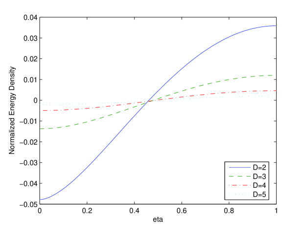
Figure 1. The normalized zero temperature free energy density $d^{D}f_{\alpha;0,\eta}^{0}$ for $D=2,3,4,5$ and $\alpha=1$. The horizontal axis is the $\eta$ axis.

When $\eta=0$, its value

$$f_{\alpha;\chi,\mu}^{0}= -\frac{\sigma_{\chi,\mu}\alpha}{d^{D}}\frac{\Gamma\left(\frac{D+1}{2}\right)}{2^{D+1}\pi^{(D+1)/2}}\zeta_{R}(D+1)$$

is negative, and when $\eta=1$, its value

$$f_{\alpha;\chi,\mu}^{0}= -\frac{\sigma_{\chi,\mu}\alpha}{d^{D}}\frac{\Gamma\left(\frac{D+1}{2}\right)}{2^{D+1}\pi^{(D+1)/2}}\sum_{n=1}^{\infty}\frac{(-1)^{n}}{n^{D+1}}$$

$$= (1-2^{-D})\frac{\sigma_{\chi,\mu}\alpha}{d^{D}}\frac{\Gamma\left(\frac{D+1}{2}\right)}{2^{D+1}\pi^{(D+1)/2}}\zeta_{R}(D+1)$$

is positive. We are going to show in the Appendix that the function

(4.7) $$\mathfrak{B}_{n}(x)=\sum_{k=1}^{\infty}\frac{\cos(2\pi kx)}{k^{n}},\hskip 28.45274pt0\leq x\leq 1,\;\;n\geq 2$$

is increasing in the interval $[0,1/2]$. Consequently, when $\eta$ changes from $0$ to $1$, the zero temperature energy density increases, and it changes from negative to positive, so that the nature of the force in the system changes accordingly from attractive to repulsive. For a specific $D$, there is a transition value $\eta_{D}$ so that the force is attractive when $\eta\in[0,\eta_{D})$ and the force is repulsive when $\eta\in(\eta_{D},1]$. We tabulate some values of $\eta_{D}$ in Table 6.1.

Table 6.1
    $D$           $\eta_{D}$     $D$        $\eta_{D}$ 2 0.4226 3          0.4617 4 0.4807 5          0.4902 6 0.4951 7          0.4975

From this table, we see that $\eta_{D}$ is an increasing function of $D$. We have verified numerically that this is true for all $D\leq 45$. On the other hand, we can in fact show mathematically that $\eta_{D}<0.5$ for all $D$ (see Appendix). In Figure 2, we show the graph of $\eta_{D}$ as a function of $D$.

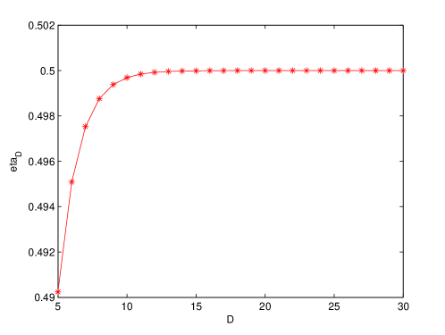
Figure 2. $\eta_{D}$ (eta_D) as a function of $D$.

From (4.4), (4.5) and (4.6), we also find that when $\chi\neq\mu$ or $(\chi,\mu)=(0,0)$, the thermal correction to the zero temperature energy decays exponentially, whereas if $\chi=\mu\neq 0$, there is a term proportional to $T^{D}$.

When $\xi\ll 1$, the dependence of the normalized free energy density on $\xi$ and $\eta=\mu-\chi$ for $D=3$ is shown in Figure 3 and Figure 4.

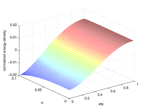
Figure 3. The normalized free energy density $d^{D}f_{\alpha;0,\eta}$ for $D=3$ and $\alpha=1$. The $x$ and $y$ axes are the $\xi$ (xi) and $\eta$ (eta) axes.

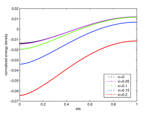
Figure 4. The normalized free energy density $d^{D}f_{\alpha;0,\eta}$ for $D=3$ and $\alpha=1$ when $\xi=0,0.05,0.1,0.15,0.2$ respectively.

4.2. High Temperature Expansion

Take $c_{1}=1/a_{2},c_{2}=1/a_{1},\mathbf{h}=(0,\eta/2)$ in (4.1), we have the high temperature ($T\gg 1$ or $\xi\gg 1$) expansion of the free energy density (3.23), .i.e.

$$f_{\alpha;\chi,\mu}= -\frac{\sigma_{\chi,\mu}\alpha d\Gamma\left(\frac{D+1}{2}\right)}{2^{D+2}\pi^{\frac{3(D+1)}{2}}}\Biggl{(}2\left(\frac{2\pi^{2}\xi}{d}\right)^{D+1}\zeta_{R}(D+1)+\frac{4\pi^{D+(5/2)}\Gamma\left(\frac{D}{2}\right)}{d^{D+1}\Gamma\left(\frac{D+1}{2}\right)}\xi\sum_{n=1}^{\infty}\frac{\cos(\pi n\eta)}{n^{D}}$$

$$+\frac{2^{(D/2)+4}\pi^{2D+(5/2)}}{d^{D+1}\Gamma\left(\frac{D+1}{2}\right)}\xi^{(D+2)/2}\sum_{n=1}^{\infty}\sum_{m=1}^{\infty}\cos(\pi n\eta)\left(\frac{m}{n}\right)^{D/2}K_{D/2}\left(4\pi^{2}mn\xi\right)\Biggr{)}.$$

Using the asymptotic expansion of the modified Bessel function (4.3), we find that if $T\gg 1$ (or equivalently $\xi\gg 1$),

(4.8) $$f_{\alpha;\chi,\mu}\sim -\frac{\sigma_{\chi,\mu}\alpha}{d^{D}}\Biggl{(}\pi^{(D+1)/2}\Gamma\left(\frac{D+1}{2}\right)\zeta_{R}(D+1)\xi^{D+1}+\frac{\Gamma\left(\frac{D}{2}\right)}{2^{D}\pi^{(D/2)-1}}\xi\sum_{n=1}^{\infty}\frac{\cos(\pi n\eta)}{n^{D}}$$

$$+\frac{\pi^{(D+1)/2}}{2^{(D-1)/2}}\cos(\pi\eta)\xi^{(D+1)/2}\left(1+\sum_{k=1}^{\infty}\frac{(D/2,k)}{(8\pi^{2}\xi)^{k}}\right)e^{-4\pi^{2}\xi}\Biggr{)}+O\left(e^{-8\pi^{2}\xi}\right).$$

The leading term

$$f_{\alpha;\chi,\mu}^{\infty,1}=-\frac{\sigma_{\chi,\mu}\alpha}{d^{D}}\pi^{(D+1)/2}\Gamma\left(\frac{D+1}{2}\right)\zeta_{R}(D+1)\xi^{D+1}$$

is proportional to $T^{D+1}$, and is independent of $\eta$. When $D=3$, it gives

$$f_{\alpha;\chi,\mu}^{\infty,1}=-\sigma_{\chi,\mu}\alpha\frac{\pi^{2}d}{90}T^{4},$$

which is called the Stefan-Boltzmann term. The next leading term of the energy density at high temperature is proportional to $T$, with proportionality constant depends on $\eta$. The rest of the terms decay exponentially. From this, we can conclude that when the temperature is large enough, the effect of different boundary conditions is not significant and the system exhibits a universal behavior regardless of the boundary conditions. When $\xi\gg 1$, the dependence of the normalized free energy density on $\xi$ and $\eta=\mu-\chi$ for $D=3$ is shown in Figure 5.

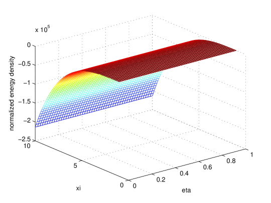
Figure 5. The normalized free energy density $d^{D}f_{\alpha;0,\eta}$ for $D=3$ and $\alpha=1$. The $x$ and $y$ axes are the $\eta$ (eta) and $\xi$ (xi) axes.

As we explain in Section 3.6, if we take $\sigma_{\chi,\mu}=2$, $\omega_{\chi,\mu}=0$, $\alpha=1$, $\eta=0$ and $D=3$ in the energy density $f_{\alpha;\chi,\mu}$ (3.23), we obtain the Casimir energy for electromagnetic fields confined between perfectly conducting parallel infinite plates (3.24). Therefore, we obtain from (4.4) and (4.8) the low and high temperature limit of the Casimir energy (3.24):

$$f_{Cas}\sim -\frac{1}{d^{3}}\Biggl{(}\frac{\pi^{2}}{720}+\frac{\pi^{2}}{2}\zeta_{R}(3)\xi^{3}+\pi^{2}\left(\xi^{2}+\xi^{3}\right)e^{-\frac{1}{\xi}}\Biggr{)}+O\left(e^{-\frac{2}{\xi}}\right),\hskip 8.5359pt\xi\ll 1,$$

$$f_{Cas}\sim -\frac{1}{d^{3}}\Biggl{(}\frac{\pi^{6}}{45}\xi^{4}+\frac{\xi}{8}\zeta_{R}(3)+\left(\pi^{2}\xi^{2}+\frac{\xi}{4}\right)e^{-4\pi^{2}\xi}\Biggr{)}+O\left(e^{-8\pi^{2}\xi}\right),\hskip 5.69046pt\xi\gg 1,$$

agree with the result of [60]. On the other hand, if we take $\sigma_{\chi,\mu}=2$, $\omega_{\chi,\mu}=0$, $\alpha=1$, $\eta=1$ and $D=3$, we obtain the Casimir energy for electromagnetic fields confined between one perfectly conducting and one infinitely permeable parallel infinite plates. Therefore, from (4.6) and (4.8), we find that the low and high temperature limits of the Casimir energy density of this system are

$$-\frac{1}{d^{3}}\Biggl{(}-\frac{7\pi^{2}}{5760}+\pi^{2}\left(\frac{\xi^{2}}{2}+\xi^{3}\right)e^{-\frac{1}{2\xi}}\Biggr{)}+O\left(e^{-\frac{1}{\xi}}\right),\hskip 28.45274pt\xi\ll 1,$$

$$-\frac{1}{d^{3}}\Biggl{(}\frac{\pi^{6}}{45}\xi^{4}-\frac{3}{32}\zeta_{R}(3)\xi-\left(\pi^{2}\xi^{2}+\frac{\xi}{4}\right)e^{-4\pi^{2}\xi}\Biggr{)}+O\left(e^{-8\pi^{2}\xi}\right),\hskip 8.5359pt\xi\gg 1.$$

These agree with the results in [33].

5. Temperature Inversion Symmetry

Since the observation of the symmetry between low and high temperature exhibited by the Casimir energy between perfectly conduction parallel plates (3.24) pointed out by Brown and Maclay in [60], there have been a number of papers devoted to the discussion of the temperature inversion symmetry of different systems [33, 34, 35, 36, 37, 38, 39]. Here we want to point out the mathematical origin of this symmetry, and show that in some particular cases, the free energy density (3.22) exhibits temperature inversion symmetry.

Observe that when $\mathbf{h}=0=\mathbf{g}$, the Epstein zeta function (3.10) is completely symmetric with respect to $a_{1}$ and $a_{2}$. In particular, if we define

$$H_{s}(w)=\sum_{(n_{1},n_{2})\in{\mathbb{Z}}^{2}}\!^{\prime}\frac{1}{\left(n_{1}^{2}+(n_{2}w)^{2}\right)^{s}}=Z_{E}(s;1,w^{2};\mathbf{0},\mathbf{0}),$$

then

$$Z_{E}(s;a_{1},a_{2};\mathbf{0},\mathbf{0})=a_{1}^{-s}H_{s}\left(\sqrt{\frac{a_{2}}{a_{1}}}\right)=a_{2}^{-s}H_{s}\left(\sqrt{\frac{a_{1}}{a_{2}}}\right).$$

The symmetry of the Epstein zeta function expressed using $H_{s}$ is the relation

(5.1) $$H_{s}(w)=w^{-2s}H_{s}\left(\frac{1}{w}\right).$$

In our case, $\sqrt{a_{2}/a_{1}}=2\pi\xi=2dT$ and formulas in the form (5.1) precisely gives a relation between low and high temperature.

Using the formula (3.23) for free energy density, when $\chi=\mu$, we have $\mathbf{g}=\mathbf{0}$ and therefore

$$d^{D}f_{\alpha;\chi,\chi}= -\frac{\sigma_{\chi,\mu}\alpha\Gamma\left(\frac{D+1}{2}\right)}{2^{D+2}\pi^{\frac{3(D+1)}{2}}}d^{D+1}a_{2}^{\frac{D+1}{2}}H_{\frac{D+1}{2}}\left(\sqrt{\frac{a_{2}}{a_{1}}}\right)-\sigma_{\chi,\mu}\omega_{\chi,\mu}\frac{\alpha\pi^{\frac{D}{2}}\Gamma\left(\frac{D}{2}\right)}{2}\xi^{D}\zeta_{R}(D).$$

The second term is zero except when $\chi=\mu=0$ or 1. The first term, denoted by $\mathcal{F}_{0}$, is a function of $\xi$ and is equal to

$$\mathcal{F}_{0}(\xi)= -\frac{\sigma_{\chi,\mu}\alpha\Gamma\left(\frac{D+1}{2}\right)\pi^{\frac{D+1}{2}}}{2}\xi^{D+1}H_{\frac{D+1}{2}}\left(2\pi\xi\right).$$

From (5.1), it satisfies the inversion symmetry

$$\mathcal{F}_{0}(\xi)=(2\pi\xi)^{D+1}\mathcal{F}_{0}\left(\frac{1}{4\pi^{2}\xi}\right).$$

For $D=3$, $\alpha=1$, this is precisely the symmetry observed in [60, 36] for electromagnetic field confined between parallel perfectly conducting plates. Therefore, when $\chi=\mu\neq 0,1$, the normalized free energy density of a massless fractional Klein-Gordon field confined between two parallel hyperplanes $d^{D}f_{\alpha;\chi,\mu}$ has a complete temperature inversion symmetry. When $\chi=\mu=0,1$, the symmetry is broken by a term proportional to $\xi^{D}\zeta_{R}(D)$.

When $\eta=\pm 1$ or equivalently, $(\chi,\mu)=(0,1)$ or $(1,0)$, from (3.23) we have

$$d^{D}f_{\alpha;0,1}= -\frac{\alpha\Gamma\left(\frac{D+1}{2}\right)}{2^{D+2}\pi^{\frac{3(D+1)}{2}}}(\sqrt{a_{1}a_{2}}d)^{D+1}\sum_{m\in{\mathbb{Z}}}\sum_{n\in{\mathbb{Z}}}\!^{\prime}\frac{(-1)^{n}}{(a_{1}m^{2}+a_{2}n^{2})^{(D+1)/2}}.$$

We can rewrite the double sum as

$$\sum_{m\in{\mathbb{Z}}}\sum_{n\in{\mathbb{Z}}}\!^{\prime}\frac{(-1)^{n}}{(a_{1}m^{2}+a_{2}n^{2})^{(D+1)/2}}$$

$$= 2\sum_{m\in{\mathbb{Z}}}\sum_{n\in{\mathbb{Z}}}\!^{\prime}\frac{1}{(a_{1}m^{2}+a_{2}(2n)^{2})^{(D+1)/2}}-\sum_{m\in{\mathbb{Z}}}\sum_{n\in{\mathbb{Z}}}\!^{\prime}\frac{1}{(a_{1}m^{2}+a_{2}n^{2})^{(D+1)/2}}.$$

Therefore, the normalized free energy density $d^{D}f_{\alpha;0,1}$ can be written as a sum of two functions in $\xi$, ${}_{1}\!\mathcal{F}_{1}(\xi)$ and ${}_{2}\!\mathcal{F}_{1}(\xi)$ where

$${}_{1}\!\mathcal{F}_{1}(\xi)= -\alpha\Gamma\left(\frac{D+1}{2}\right)\pi^{\frac{D+1}{2}}\xi^{D+1}H_{\frac{D+1}{2}}\left(4\pi\xi\right),$$

$${}_{2}\!\mathcal{F}_{1}(\xi)= \frac{\alpha}{2}\Gamma\left(\frac{D+1}{2}\right)\pi^{\frac{D+1}{2}}\xi^{D+1}H_{\frac{D+1}{2}}\left(2\pi\xi\right).$$

Using (5.1), we find that each of these functions satisfies an inversion symmetry

$${}_{1}\!\mathcal{F}_{1}(\xi)=(4\pi\xi)^{D+1}\;_{1}\!\mathcal{F}_{1}\left(\frac{1}{16\pi^{2}\xi}\right),\hskip 28.45274pt_{2}\!\mathcal{F}_{1}(\xi)=(2\pi\xi)^{D+1}\;_{2}\!\mathcal{F}_{1}\left(\frac{1}{4\pi^{2}\xi}\right).$$

When $D=3$, $\alpha=1$, this is what observed in [33] for electromagnetic field confined between parallel plates under Boyer’s setup.

For generic $\eta$, there was no temperature inversion symmetry since the components in $\mathbf{g}$ are not symmetric. However, for some particular rational values of $\eta$, we can use the same trick as in the case $\eta=1$ and write the normalized energy density as a sum of a few functions such that each of them has temperature inversion symmetry. For example, when $\eta=2/3$, using the fact that when $f(x)$ is an even function,

$$\sum_{n\in{\mathbb{Z}}}e^{\pi in\eta}f(n)= f(0)+2\Biggl{(}\sum_{n\geq 1,n\equiv 0\;\text{mod}\;3}f(n)+\sum_{n\geq 1,n\equiv 1\;\text{mod}\;3}\cos\left(\frac{2\pi}{3}\right)f(n)$$

$$\hskip 85.35826pt+\sum_{n\geq 1,n\equiv 2\;\text{mod}\;3}\cos\left(\frac{4\pi}{3}\right)f(n)\Biggr{)}$$

$$= f(0)+3\sum_{n\geq 1,n\equiv 0\;\text{mod}\;3}f(n)-\sum_{n=1}^{\infty}f(n)$$

$$= \frac{3}{2}\sum_{n\in{\mathbb{Z}}}f(3n)-\frac{1}{2}\sum_{n\in{\mathbb{Z}}}f(n),$$

we can write $d^{D}f_{\alpha;\chi,\chi\pm(2/3)}$ as a sum of two functions ${}_{1}\!\mathcal{F}_{2}(\xi)$, ${}_{2}\!\mathcal{F}_{2}(\xi)$ given by

$${}_{1}\!\mathcal{F}_{2}(\xi)= -\frac{3}{2}\alpha\Gamma\left(\frac{D+1}{2}\right)\pi^{\frac{D+1}{2}}\xi^{D+1}H_{\frac{D+1}{2}}\left(6\pi\xi\right),$$

$${}_{2}\!\mathcal{F}_{2}(\xi)= \frac{\alpha}{2}\Gamma\left(\frac{D+1}{2}\right)\pi^{\frac{D+1}{2}}\xi^{D+1}H_{\frac{D+1}{2}}\left(2\pi\xi\right).$$

Each of these functions satisfies temperature inversion symmetry

$${}_{1}\!\mathcal{F}_{2}(\xi)=(6\pi\xi)^{D+1}\;_{1}\!\mathcal{F}_{2}\left(\frac{1}{36\pi^{2}\xi}\right),\hskip 28.45274pt_{2}\!\mathcal{F}_{2}(\xi)=(2\pi\xi)^{D+1}\;_{2}\!\mathcal{F}_{2}\left(\frac{1}{4\pi^{2}\xi}\right).$$

6. Conclusion

We have introduced a new type of boundary condition called fractional Neumann condition which involves vanishing fractional derivative of the field in the study of Casimir effect of fractional massless Klein-Gordon field confined between a pair of parallel plates. By imposing this fractional Neumann conditions on the plates allows the interpolation between the usual Dirichlet and Neumann conditions. Our results indicate that there exists a transition value for the difference between the orders of the fractional Neumann conditions in the two plates for which the Casimir force changes from attractive to repulsive (or vice versa). It is interesting to note that for sufficiently high temperature, the Hemholtz free energy density is dominated by a term independent of boundary conditions. Conditions for temperature inversion symmetry to hold are also discussed.

We would also like to point out that despite a few decades of work on temperature dependence of Casimir effect, there still exist debates on this topic. The main issue of the recent controversy lies in the thermodynamic consistency of the computed Casimir force between real metals and the Drude dispersion relation (see references [64, 65, 66, 67, 68] for both sides of the controversy). It has to do with the controversy of inclusion/exclusion of the TE (transverse electric) zero mode. Some authors [69, 70, 71] claimed that the Drude relation does not provide a consistent explanation of recent experimental results, in particular it is in conflict with the Nernst theorem. They proposed to replace the Drude relation by the plasma relation. On the other hand, Hoye, Brevik, Aarseth, Ellingsen and Milton [65, 67, 72, 73, 74, 75, 76, 77, 78] have argued in favor of the exclusion of the TE zero mode. They have derived analytical results using Euler-Maclaurin formula, which in the limit $T\rightarrow 0$ are consistent with the Nernst theorem [79]. They have also carried out numerical calculation of the free energy and obtained results which agree with analytic results to a high degree of accuracy. These authors also proposed an experimental setup to test such results [78]. We plan to discuss in detail the Casimir energy of fractional electromagnetic field and the issue of inclusion/exclusion of the TE zero mode in a future work.

Finally, we would like to suggest some other possible directions for further work. The extension of our discussion to a $p$–dimensional cavity embedded in $D$–dimensional space, with $p\leq D$ is currently under consideration. However for the generalization of the above results to non-flat space is likely to encounter highly non-trivial mathematical problems since one needs to deal with fractional operators in curved space. Another interesting generalization involves fractional Klein-Gordon field with fractional Neumann boundary conditions of variable fractional order, which allows variable Casimir energy or force at different point in space. Such a problem again requires results from derivatives and integrations of fractional variable order, a subject which is still at its infancy.

Acknowledgement  S.C. Lim and L.P. Teo would like to thank Malaysian Academy of Sciences, Ministry of Science, Technology and Innovation for funding this project under the Scientific Advancement Fund Allocation (SAGA) Ref. No P96c.

Appendix A The Function $\mathfrak{B}_{n}(x)$

In this appendix, we are going to show that the function (4.7)

$$\mathfrak{B}_{n}(x)=\sum_{k=1}^{\infty}\frac{\cos(2\pi kx)}{k^{n}}$$

is increasing and has exactly one zero in the interval $[0,1/2]$. We are also going to show that this unique zero is less than $1/4$.

First, we show that $\mathfrak{B}_{n}(x)$ is increasing and has exactly one zero in the interval $[0,1/2]$. As a matter of fact, for $n$ even, the function $\mathfrak{B}_{n}(x)$ is well known. From 9.622 of [57], we have

(A.1) $$\mathfrak{B}_{2n}(x)=(-1)^{n-1}\frac{(2\pi)^{2n}}{2(2n)!}B_{2n}(x),\hskip 28.45274pt0\leq x\leq 1,$$

where $B_{k}(x)$ is the $k$-th Bernoulli polynomial defined by

$$\frac{te^{tx}}{e^{t}-1}=\sum_{k=0}^{\infty}\frac{B_{k}(x)}{k!}t^{k}.$$

The explicit formula for $B_{k}(x)$ for $1\leq k\leq 5$ is given in Table A.1.

Table A.1
    $k$    $B_{k}(x)$ 1    $x-\frac{1}{2}$ 2    $x^{2}-x+\frac{1}{6}$ 3     $x^{3}-\frac{3}{2}x^{2}+\frac{1}{2}x$ 4 $x^{4}-2x^{3}+x^{2}-\frac{1}{30}$ 5 $x^{5}-\frac{5}{2}x^{4}+\frac{5}{3}x^{3}-\frac{1}{6}x$

It is well known that for all $k\geq 1$, $B_{k+1}^{\prime}(x)=(k+1)B_{k}(x)$. From 9.622 of [57] again, we have

(A.2) $$B_{2n-1}(x)=\frac{(-1)^{n}2(2n-1)!}{(2\pi)^{2n-1}}\sum_{k=1}^{\infty}\frac{\sin(2k\pi x)}{k^{2n-1}},\hskip 28.45274pt\begin{cases}k=1,&0<x<1\\ k\geq 2,&0\leq x\leq 1\end{cases}.$$

From this it is easy to verify that $B_{2n}(x)$ is increasing and has exactly one zero in the interval $[0,1/2]$ (see e.g. [80]). For convenience, we repeat the argument here. As is easily verify from (A.1),

$$B_{2n}(0)= 2(-1)^{n-1}\frac{(2n)!}{(2\pi)^{2n}}\zeta_{R}(2n),$$

$$B_{2n}(1/2)= 2(1-2^{1-2n})(-1)^{n}\frac{(2n)!}{(2\pi)^{2n}}\zeta_{R}(2n),$$

which shows that $B_{2n}(0)$ and $B_{2n}(1/2)$ has opposite sign and is nonzero. It also implies that $B_{2n}(x)$ must has at least one zero in $[0,1/2]$. On the other hand, we find from (A.2) that $B_{2k+1}(0)=B_{2k+1}(1/2)=0$ for all $k\geq 1$. Now if for some $j\geq 1$, $B_{2j}(x)$ has two zeros in $[0,1/2]$, then its derivative $2jB_{2j-1}(x)$ has a zero in $(0,1/2)$. Since $B_{2j-1}(0)=B_{2j-1}(1/2)=0$, this in turn implies that its derivative $(2j-1)B_{2j-2}(x)$ has two zeros in $[0,1/2]$. Continuing this argument, we find that $B_{1}(x)$ must have a zero in $(0,1/2)$. This gives a contradiction since $B_{1}(x)=x-(1/2)$ does not have any zero in $(0,1/2)$. This shows that $B_{2n}(x)$ has exactly one zero in the interval $[0,1/2]$ and $B_{2n-1}(x)$ does not have any zero in the open interval $(0,1/2)$. The latter implies that $B_{2n-1}(x)$ must be either always nonnegative or always nonpositive in the interval $(0,1/2)$. Therefore, $B_{2n}(x)$ is monotone in $[0,1/2]$. This completes our argument for $\mathfrak{B}_{2n}(x)$.

To verify the statement for $\mathfrak{B}_{2n-1}(x)$, $n\geq 1$, we define the functions

$$\mathfrak{D}_{n}(x)=\sum_{k=1}^{\infty}\frac{\sin(2k\pi x)}{k^{n}},\hskip 28.45274pt\begin{cases}n=1,&0<x<1\\ n\geq 2,&0\leq x\leq 1\end{cases}$$

and let

$$C_{2n-1}(x)=\frac{(-1)^{n-1}}{(2\pi)^{2n-1}}\mathfrak{B}_{2n-1}(x),\hskip 28.45274ptC_{2n}(x)=\frac{(-1)^{n-1}}{(2\pi)^{2n}}\mathfrak{D}_{2n}(x)$$

for all $n\geq 1$. Then it is easy to verify that $C_{n+1}^{\prime}(x)=C_{n}(x)$. Moreover, for all $n\geq 1$,

$$C_{2n+1}(0)= \frac{(-1)^{n}}{(2\pi)^{2n+1}}\zeta_{R}(2n+1),$$

$$C_{2n+1}(1/2)= -(1-2^{-2n})\frac{(-1)^{n}}{(2\pi)^{2n+1}}\zeta_{R}(2n+1),$$

$C_{2n}(0)=C_{2n}(1/2)=0$. On the other hand, for $0<x<1$,

$$\mathfrak{B}_{1}(x)+i\mathfrak{D}_{1}(x)=\sum_{k=1}^{\infty}\frac{e^{2\pi ikx}}{k}=-\log\left(1-e^{2\pi ix}\right)=-\log(2\sin(\pi x))-i\pi\left(x-\frac{1}{2}\right).$$

Therefore,

$$C_{1}(x)=\frac{1}{2\pi}\mathfrak{B}_{1}(x)=-\frac{1}{2\pi}\log(2\sin(\pi x))$$

and it is easy to verify that $C_{1}(x)$ is decreasing on $(0,1/2)$, positive on $(0,1/6)$, negative on $(1/6,1/2]$ and zero at $x=1/6$. Since $C_{2}^{\prime}(x)=C_{1}(x)$, we find that $C_{2}$ is strictly increasing on $[0,1/6]$ and strictly decreasing on $[1/6,1/2]$. Since $C_{2}(0)=C_{2}(1/2)=0$, $C_{2}(x)>0$ for all $x\in(0,1/2)$. The same argument used for $B_{2n}$ then shows that $C_{2n+1}(x)$ is monotone and has exactly one zero in the interval $[0,1/2]$, thus verifying the statement for $\mathfrak{B}_{2n-1}(x)$.

Now since $\mathfrak{B}_{n}(0)=\zeta_{R}(n)>0$, $\mathfrak{B}_{n}(1/2)=-(1-2^{1-n})\zeta_{R}(n)<0$, to show that the unique zero of $\mathfrak{B}_{n}(x)$ is less than $1/4$, it is enough to show that $\mathfrak{B}_{n}(1/4)<0$. A straightforward computation gives

$$\mathfrak{B}_{n}\left(\frac{1}{4}\right)=-\frac{1}{2^{n}}+\frac{1}{4^{n}}-\frac{1}{6^{n}}+\frac{1}{8^{n}}+\ldots=\frac{1}{2^{n}}\mathfrak{B}_{n}\left(\frac{1}{2}\right)<0,$$

verifying our claim.

References

- [1] R. Hilfer (Ed.), Applications of Fractional Calculus in Physics, World Scientific, Singapore, (2000).
- [2] G. M. Zaslavsky, Chaos, fractional kinetics, and anomalous transport, Phys. Rep. 371 (2002), 461–580.
- [3] B. J. West, M. Bologna and P. Grigolini, Physics of Fractal Operators, Springer–Verlag, New York, (2003).
- [4] R. Metzler and J. Klafter, The restaurant at the end of the random walk: recent developments in the description of anomalous transport by fractional dynamics, J. Phys. A 37 (2004), R161–R208.
- [5] L. M. Zelenyi and A. V. Milovanov, Fractal topology and strange kinetics: from percolation theory to problems in cosmic electrodynamics, Phys. Uspekhi 47 (2004), no. 8, 749–788.
- [6] G. M. Zaslavsky, Hamiltonian Chaos and Fractional Dynamics, Oxford University, Oxford, (2005).
- [7] N. Laskin, Fractional quantum mechanics, Phys. Rev. E 62 (2000), 3135–3145.
- [8] N. Laskin, Fractals and quantum mechanics, Chaos 10 (2000), 780–790.
- [9] N. Laskin, Fractional Schrodinger equation, Phys. Rev. E 66 (2002), Art. No. 056108.
- [10] M. Naber, Time fractional Schrodinger equation, J. Math. Phys. 45 (2004), 3339–3352.
- [11] X. Guo and M. XU, Some physical applications of fractional Schrodinger equation, J. Math. Phys. 47 (2006), Art. No. 082104.
- [12] C. G. Bollini and J. J. Giambiagi, Arbitrary powers of d’Alembertians and the Huygens principle, J. Math. Phys. 34 (1993), no. 2, 610–621.
- [13] Claus Lämmerzahl, The pseudodifferential operator square root of the Klein-Gordon equation, J. Math. Phys. 34 (1993), no. 9, 3918–3932.
- [14] S. Albeverio H. Gottschalk and J.-L Wu, Convoluted generalized white noise, Schwinger functions and their analytic continuation to Wightman functions, Rev. Math. Phys. 8 (1996), 763–817.
- [15] M. Grothaus and L. Streit, Construction of relativistic quantum fields in the framework of white noise analysis, J. Math. Phys. 40 (1999), 5387–5405.
- [16] M. S. Plyushchay and Michel Rausch de Traubenberg, Cubic root of Klein-Gordon equation, Phys. Lett. B 477 (2000), no. 1-3, 276–284.
- [17] A. Raspini, Simple solutions of the fractional Dirac equation of order 2/3, Physica Scripta 64 (2001), 20–22.
- [18] Petr Závada, Relativistic wave equations with fractional derivatives and pseudodifferential operators, J. Appl. Math. 2 (2002), no. 4, 163–197.
- [19] R. L. P. G. do Amaral and E. C. Marino, Canonical quantization of theories containing fractional powers of the d’Alembertian operator, J. Phys. A 25 (1992), no. 19, 5183–5200.
- [20] D. G. Barci, L. E. Oxman, and M. Rocca, Canonical quantization of nonlocal field equations, Internat. J. Modern Phys. A 11 (1996), no. 12, 2111–2126.
- [21] S. C. Lim and S. V. Muniandy, Stochastic quantization of nonlocal fields, Phys. Lett. A 324 (2004), no. 5-6, 396–405.
- [22] S. C. Lim, Fractional derivative quantum fields at positive temperature, Phys. A 363 (2006), no. 2, 269–281.
- [23] A.G. Riess et al. [Supernova Search Team Collaboration], Observational evidence from supernovae for an accelerating universe and a cosmological constant, Astron. J. 116 (1998), 1009–1038.
- [24] S. Perlmutter et al. [Suernova Cosmology Project Collaboration], Measurements of Omega and Lambda from 42 high-redshift supernovae, Astrophys. J. 517 (1999), 565–586.
- [25] J.L. Tonry et al. [Supernova Search Team Collaboration], Cosmological results from high-z supernovae, Astrophys. J. 594 (2003), 1–24.
- [26] A.G. Riess et al. [Supernova Search Team Collaboration], Type Ia supernova discoveries at from the Hubble Space Telescope: Evidence for past deceleration and constraints on dark energy evolution, Astrophys. J. 607 (2004), 665–687.
- [27] P.W. Milonni, The Quantum Vacuum, Academic Press, New York, (1994).
- [28] K.A. Milton, The Casimir Effect, World-Scientific, Singapore, (2001)
- [29] K.A. Milton, Dark Energy as Evidence for Extra Dimensions, Grav. Cosmol. 9 (2003), 66–70.
- [30] P. Brax, J. Martin, J-P Uzan, Eds. On the Nature of Dark Energy, Proceedings of 18th IAP Astrophysics Colloquium, Frontier Group, (2002).
- [31] T.H. Boyer, Van der Waals forces and zero-point energy for dielectric and permeable materials, Phys. Rev. A 9 (1974), 2078–2084.
- [32] M.V. Cougo-Pinto, C. Farina, J.F.M. Mendes and A.C. Tort, zeta-function method for repulsive Casimir forces, Braz. J. Phys. 29 (1999), 371–374.
- [33] F. C. Santos, A. Tenorio and A. C. Tort, Zeta function method and repulsive Casimir forces for an unusual pair of plates at finite temperature, Physical Review D 60 (1999), no. 10, Art. No. 105022.
- [34] S. Tadaki and S. Takagi, Casimir Effect at Finite Temperature, Prog. Theor. Phys. 75 (1982), 262–271.
- [35] S.A. Gundersen and F. Ravndal, The Fermionic Casimir effect at finite temperature, Ann. Phys. (N.Y.) 182 (1988), 90–111.
- [36] F. Ravndal and D. Tollefsen, Temperature inversion symmetry in the Casimir effect, Physical Review D 40 (1989), no. 12, 4191–4192.
- [37] by same author, On the Casimir effect and the temperature inversion symmetry, J. Phys. A 23 (1990), no. 9, 1627–1632.
- [38] C. Wotzasek, A symmetry in the finite-temperature Casimir effect, J. Phys. A 21 (1988), L793–L796.
- [39] A. C. Aguiar Pinto, T. M. Britto, F. Pascoal, and F. S. S. da Rosa, Temperature inversion symmetry in the Casimir effect with an antiperiodic boundary condition, Phys. Rev. D 67 (2003), Art. No. 107701.
- [40] Hitoshi Kumano-go, Pseudodifferential operators, MIT Press, Cambridge, Mass., (1981).
- [41] S. Samko, A.A. Kilbas and D.I. Maritchev, Integrals and Derivatives of the Fractional Order and Some of Their Applications, Gordon and Breach, Armsterdam, (1993).
- [42] C. G. Bollini and J.J. Giambiagi, Lagrangian procedures for higher order field equations, Revista Brasileira de Fsica 17 (1987), no. 1, 14–30.
- [43] A. Pais and G. E. Uhlenbeck, On field theories with non-localized action, Physical Rev. (2) 79 (1950), 145–165.
- [44] E. C. Marino, Complete bosonization of the Dirac fermion field in dimensions, Phys. Lett. B 263 (1991), no. 1, 63–68.
- [45] D.G. Barci, César D. Fosco, and L.E. Oxman, On bosonization in dimensions, Phys. Lett. B375 (1996), no. 1, 267–272.
- [46] A. O. Barvinsky and G. A. Vilkovisky, Beyond the Schwinger-DeWitt technique: Converting loops into trees and in-in currents, Nucl. Phys. B282 (1987), 163–188; Covariant perturbation theory. II. Second order in the curvature. General algorithms, Nucl. Phys. B333 (1990), no. 2, 471–511.
- [47] Diego A. R. Dalvit and Francisco D. Mazzitelli, Running coupling constants, Newtonian potential, and nonlocalities in the effective action, Phys. Rev. D 50 (1994), no. 2, 1001–1009.
- [48] L. Nottale, Fractal Space-Time and Microphysics, World Scientific, Singapore, (1993).
- [49] H. Kroger, Fractal geometry in quantum mechanics, field theory and spin systems, Phys. Rep. 323 (2000), 82–181.
- [50] J.S. Dowker and R. Critchley, Effective Lagrangian and energy-momentum tensor in deSitter space, Phys. Rev. D13 (1976), 3224–3232.
- [51] S.W. Hawking, Zeta function regularization of path integrals in curved spacetime, Commun. Math. Phys. 55 (1977), 133–148.
- [52] G.W. Gibbons, Thermal zeta functions, Phys. Lett. A60 (1977), 385–386.
- [53] Jan Ambjørn and S. Wolfram, Properties of the vacuum. I. Mechanical and thermodynamic, Ann. Physics 147 (1983), 1–32.
- [54] E. Elizalde, S. D. Odintsov, A. Romeo, A. A. Bytsenko, and S. Zerbini, Zeta regularization techniques with applications, World Scientific Publishing Co. Inc., River Edge, NJ, 1994.
- [55] Emilio Elizalde, Ten physical applications of spectral zeta functions, Lecture Notes in Physics. New Series m: Monographs, vol. 35, Springer-Verlag, Berlin, 1995.
- [56] K. Kirsten, Spectral functions in mathematics and physics, Chapman & Hall/ CRC, Boca Raton, FL, 2002.
- [57] I. S. Gradshteyn and I. M. Ryzhik, Table of integrals, series, and products, sixth ed., Academic Press Inc., San Diego, CA, 2000, Translated from the Russian.
- [58] G. Barton, Quantum electrodynamics of spinless particles between conducting plates, Proc. R. Soc. Lond. 320 (1970), no. 1541, 251–275.
- [59] C. Farina, Casimir effect: some aspects, Braz. J. Phys. 36 (2006), 1137–1149.
- [60] Lowell S. Brown and G. Jordan Maclay, Vacuum stress between conduction plates: an image solution, Physical Review 184 (1969), no. 5, 1272–1279.
- [61] E. Elizalde, An extension of the Chowla-Selberg formula useful in quantizing with the Wheeler-DeWitt equation, J. Phys. A 27 (1994), no. 11, 3775–3785.
- [62] by same author, Zeta functions: formulas and applications, J. Comput. Appl. Math. 118 (2000), no. 1-2, 125–142, Higher transcendental functions and their applications.
- [63] George E. Andrews, Richard Askey, and Ranjan Roy, Special functions, Encyclopedia of Mathematics and its Applications, vol. 71, Cambridge University Press, Cambridge, 1999.
- [64] R. S. Decca, D. Lopez, E. Fischbach et al, Precise comparison of theory and new experiment for the Casimir force leads to stronger constraints on thermal quantum effects and long-range interactions, Ann. Phys. 318 (2005), no. 1, 37–80.
- [65] I. Brevik, J. B. Aarseth, J. S. Høye et al, Temperature dependence of the Casimir effect, Phys. Rev. E 71 (2005), no. 5, Art. No. 056101.
- [66] V. B. Bezerra, R. S. Decca, E. Fischbach et al, Comment on ”Temperature dependence of the Casimir effect”, Phys. Rev. E 73 (2006), no. 2, Art. No. 028101.
- [67] J. S. Høye, I. Brevik, J. B. Aarseth et al, What is the temperature dependence of the Casimir effect? J.Phys. A 39 (2006), no. 20, 6031–6038.
- [68] V. M. Mostepanenko, V. B. Bezerra, R. S. Decca et al, Present status of controversies regarding the thermal Casimir force, J. Phys. A 39 (2006), no. 21, 6589–6600.
- [69] G. L. Klimchitskaya, V. M. Mostepanenko, Investigation of the temperature dependence of the Casimir force between real metals, Phys. Rev. A 63 (2001), no. 6, Art. No. 062108.
- [70] M. Bordag, B. Geyer B, G. L. Klimchitskaya et al, Casimir force at both nonzero temperature and finite conductivity, Phys. Rev. Lett. 85, (2000), no. 3, 503–506.
- [71] E. Fischbach, D. E. Krause, V. M. Mostepanenko et al, New constraints on ultrashort-ranged Yukawa interactions from atomic force microscopy, Phys. Rev. D 64 (2001), no. 7, Art. No. 075010.
- [72] J. S. Høye, I. Brevik, J. B. Aarseth et al, Does the transverse electric zero mode contribute to the Casimir effect for a metal? Phys. Rev E 67 (2003), no. 5, Art. No. 056116.
- [73] M. Bostrom, B. E. Sernelius, Thermal effects on the Casimir force in the 0.1–5 m range, Phys. Rev. Lett. 84 (2000), no. 20, 4757–4760.
- [74] I. Brevik, J. B. Aarseth, Temperature dependence of the Casimir effect, J. Phys. A 39 (2006), no. 21, 6187–6193.
- [75] I. Brevik, J. B. Aarseth, J. S. Hoye, and K. A. Milton, Temperature dependence of the Casimir force for metals, in Qunatum field theory under the influence of external conditions, edited by K. A. Milton, Rinton Press, Princeton, NJ, 2004, 54–65.
- [76] I. Brevik, S. A. Ellingsen and K. A. Milton, Thermal corrections to the Casimir effect, New J. Phys. 8 (2006), Art. No. 236.
- [77] S. A. Ellingsen, Casimir attraction in multilayered plane parallel magnetodielectric systems, J. Phys. A 40, no. 9, 1951–1961.
- [78] S. A. Ellingsen and I. Brevik, Casimir force on real materials - the slab and cavity geometry, J. Phys. A 40 (2007), no. 13, 3643–3664.
- [79] J. S. Høye, I. Brevik, S. A. Ellingsen and J. B. Aarseth et al, Analytical and numerical verification of the Nernst theorem for metals, preprint arXiv:quant-ph/0703174 (2007).
- [80] H. M. Edwards, Riemann’s zeta function, Dover Publications Inc., Mineola, NY, (2001).