Theory of inelastic lifetimes of surface-state electrons and holes at metal surfaces

Abstract

After the early suggestion by John Pendry to probe unoccupied bands at surfaces through the time reversal of the photoemission process, the inverse-photoemission technique yielded the first conclusive experimental evidence for the existence of image-potential bound states at metal surfaces and has led over the last two decades to an active area of research in condensed-matter and surface physics. Here we describe the current status of the many-body theory of inelastic lifetimes of these image-potential states and also the Shockley surface states that exist near the Fermi level in the projected bulk band gap of simple and noble metals. New calculations of the self-energy and lifetime of surface states on Au surfaces are presented as well, by using the $GW\Gamma$ approximation of many-body theory.

I Introduction

In a pioneering paper pendry1 , Echenique and Pendry investigated the observability of Rydberg-like electronic states trapped at metal surfaces via low-energy electron diffraction (LEED) experiments. They discussed the lifetime broadening of these image-potential-induced surface states (image states), and reached the important conclusion that they could, in principle, be resolved for all members of the Rydberg series.

A few years later, Pendry suggested a new experiment pendry2 : measurement of the bremsstrahlung-radiation spectrum from electrons, with energies no more than a few tens of electron volts, incident on clean surfaces, thereby turning incident electrons into emitted photons. This photon-emission experiment is simply the time reversal of the photoemission process and was referred to by Pendry as inverse photoemission, or IPE for short.

Subsequently, Johnson and Smith johnson1 pointed out that image states were potentially observable by angle-resolved IPE; using this technique, Dose et al. dose1 and Straub and Himpsel straub1 reported the first conclusive experimental evidence for image-potential bound states at the (100) surfaces of copper and gold. Since then, several observations of image states have been made using this technique ip1 ; ip2 ; ip3 ; ip4 ; ip5 ; ip6 ; ip7 , and also the more recent high-resolution techniques of two-photon photoemission (2PPE) tppe1 ; tppe2 ; tppe3 and time-resolved two-photon photoemission (TR-2PPE) tppe4 ; tppe5 ; tppe6 . In 2PPE, intense laser radiation is used to populate an unoccupied state with the first photon and to photoionize from the intermediate state with the second photon. In TR-2PPE, the probe pulse which ionizes the intermediate state is delayed with respect to the pump pulse which populates it, thus providing a direct measurement of the intermediate-state lifetime.

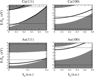
Figure 1: The $\Gamma L$ projected bulk band structure (shaded areas) of the (111) and (100) surfaces of the noble metals Cu and Au. The solid lines represent Shockley ($n=0$) and image-potential ($n=1$) surface-state bands. Well-defined Shockley states are only present at the Cu(111) and Au(111) surfaces, where the projected band gap extends below the Fermi level. Well-defined image states are present at the Cu(100) and Au(100) surfaces, and also at the (111) surface of Cu. At Au(111) there is only an image-state resonance lying above the top of the band gap. The horizontal thin solid lines represent Fermi and vacuum levels.

At metal surfaces, in addition to image states (which are originated in the combination of the long-range image potential in front of solid surfaces with the presence of a band gap near the vacuum level) image1 ; image2 there exist crystal-induced surface states (which would occur even for a step barrier in the absence of the image potential) ss often classified as Shockley and Tamm states shockley ; tamm : Shockley states exist near the Fermi level in the projected bulk band gap of simple and noble metals, and Tamm states exist at the $\bar{M}$ points of the surface Brillouin zone for various noble-metal surfaces. The lifetimes of excited holes at the band edge (${\bf k}_{\parallel}=0$) of Shockley states have been investigated with high-resolution angle-resolved photoemission (ARP) arp1 ; arp2 ; arp3 ; arp4 and with the use of the scanning tunneling microscope (STM) stm1 ; science . STM techniques have also allowed the determination of the lifetimes of excited Shockley and image electrons over a range of energies above the Fermi level stm2 ; stm3 .

Figure 1 illustrates Shockley and image-potential states in the gap of the $\Gamma L$ projected band structure of the (100) and (111) surfaces of the noble metals Cu and Au. If an electron or hole is added to the solid at one of these states, inelastic coupling of the excited quasiparticle with the crystal may occur through electron-electron (e-e) and electron-phonon (e-ph) scattering.

In this paper, we first give a brief description of existing calculations of e-ph inelastic linewidths of image and Shockley states, and we then focus on the many-body theory of e-e inelastic lifetimes of these states. In particular, we describe the current status of many-body $GW$ and $GW\Gamma$ calculations, and we report new $GW\Gamma$ calculations of the self-energy and lifetime of surface states on Au surfaces. We conclude that short-range exchange-correlation (xc) contributions to the electron (or hole) self-energy are small, as occurs in the case of bulk states.

Unless otherwise is stated, atomic units are used throughout, i. e., $e^{2}=\hbar=m_{e}=1$. The atomic unit of length is the Bohr radius, $a_{0}=\hbar^{2}/m_{e}^{2}=0.529{\rm\AA}$, the atomic unit of energy is the Hartree, $1\,{\rm Hartree}=e^{2}/a_{0}=27.2\,{\rm eV}$, and the atomic unit of velocity is the Bohr velocity, $v_{0}=\alpha\,c=2.19\times 10^{8}{\rm cm\,s^{-1}}$, $\alpha$ and $c$ being the fine-structure constant and the velocity of light, respectively.

II Electron-phonon coupling

The decay rate due to the e-ph interaction, which is relatively important only in the case of excited Shockley holes near the Fermi level, has been investigated by using the Eliashberg function grimvall . In particular, at zero temperature ($T=0$) and in the high-temperature limit ($k_{B}T>>\omega_{m}$, $k_{B}$ being Boltzmann’s constant and $\omega_{m}$, the maximum phonon frequency) one finds respectively, assuming translational invariance in the plane of the surface, the following expressions for the e-ph induced linewidth (or lifetime broadening) $\Gamma_{ep}$ of surface states of parallel momentum ${\bf k}$ and energy $E$ grimvall ; eiguren1 :

$$\Gamma_{ep}^{0}({\bf k},E)=2\pi\int_{0}^{{\rm max}(|E|,\omega_{m})}\alpha^{2}F_{\bf k}(\omega)d\omega$$ (1)

and

$$\Gamma_{ep}({\bf k},E)=2\pi\,\lambda({\bf k})\,k_{B}T,$$ (2)

where $\alpha^{2}F_{\bf k}(\omega)$ is the Eliashberg function, which represents a weighted phonon density of states, and

$$\lambda({\bf k})=\int_{0}^{\omega_{m}}{\alpha^{2}F_{\bf k}(\omega)\over\omega}d\omega.$$ (3)

For many years, the e-ph contribution $\Gamma_{ep}({\bf k},E)$ to the inelastic decay of surface states had been calculated using a three-dimensional (3D) Debye phonon model with $\lambda$ obtained from measurements or calculations of bulk properties grimvall . More refined calculations, which are based on an accurate description of the full Eliashberg spectral function, have been carried out recently by Eiguren et al. eiguren2 ; eiguren3 for (i) the Shockley surface-state hole ($n=0$) at the $\bar{\Gamma}$ point of Al(100) and the (111) surfaces of the noble metals Cu, Ag, and Au eiguren2 , and (ii) the first ($n=1$) image-state electron at the $\bar{\Gamma}$ point of the (100) surfaces of Cu and Ag eiguren3 ; these calculations are based on the use of (i) Thomas-Fermi screened Ashcroft electron-ion pseudopotentials, (ii) single-particle states obtained by solving a single-particle model one-dimensional (1D) Schrödinger equation, and (iii) a simple force-constant phonon model calculation that yields a phonon spectrum in good agreement with experimental data.

Table 1: Electron-phonon linewidths at $T=0$ ($\Gamma_{ep}^{0}$), in meV, and the parameter $\lambda$ that is responsible for the high-temperature behaviour of $\Gamma_{ep}$, as reported at the $\bar{\Gamma}$ point in Refs. eiguren2 ; eiguren3 .

Surface	$n$	$\Gamma_{ep}^{0}$	$\lambda$
Al(100)	0	18	0.23
Cu(111)	0	7.3	0.16
Ag(111)	0	3.7	0.12
Au(111)	0	3.6	0.11
Cu(100)	1	$<1\,{\rm meV}$	$<0.01$
Ag(100)	1	$<1\,{\rm meV}$	$<0.01$

A summary of the results reported by Eiguren et al. eiguren2 ; eiguren3 is presented in Table 1. Electron-phonon linewidths are particularly relevant in the case of surface-state holes with energies very near the Fermi level, in which case the contribution from e-e interactions is very small. In the case of image states, whose energies lie typically a few electronvolts above the Fermi level, the e-ph linewidth is found to be $\Gamma_{ep}<1\,{\rm meV}$, thereby showing the negligibly small role of phonons in the electron dynamics of image-potential states.

III Electron-electron coupling

Let us consider an arbitrary many-electron system of density $n_{0}({\bf r})$. In the framework of many-body theory, the e-e linewidth (or decay rate) $\Gamma_{ee}$ of a quasiparticle (electron or hole) that has been added in the single-particle state $\psi_{i}({\bf r})$ of energy $\varepsilon_{i}$ is obtained as the projection of the imaginary part of the self-energy $\Sigma({\bf r},{\bf r}^{\prime};\varepsilon_{i})$ over the quasiparticle-state itself review1 ; review2 :

$$\Gamma_{ee}=\mp 2\int d{\bf r}\int d{\bf r}^{\prime}\psi^{*}_{i}({\bf r}){\rm Im}\Sigma({\bf r},{\bf r}^{\prime};\varepsilon_{i})\psi_{i}({\bf r}^{\prime}),$$ (4)

where the $\mp$ sign in front of the integral should be taken to be minus or plus depending on whether the quasiparticle is an electron ($\varepsilon_{i}\geq\varepsilon_{F}$) or a hole ($\varepsilon_{i}\leq\varepsilon_{F}$), respectively, $\varepsilon_{F}$ being the Fermi energy. Alternatively, Eq. (4) can be written as follows

$$\Gamma_{ee}=\mp{2\over\pi}\int_{\varepsilon_{i}-0^{+}}^{\varepsilon_{i}+0^{+}}\int d{\bf r}\int d{\bf r}^{\prime}g^{0}({\bf r},{\bf r}^{\prime};\varepsilon)\,{\rm Im}\Sigma({\bf r},{\bf r}^{\prime};\varepsilon_{i}),$$ (5)

where

$$g^{0}({\bf r},{\bf r}^{\prime};\varepsilon)={i\over 2}\left\{G^{0}({\bf r}^{\prime},{\bf r};\varepsilon)-\left[G^{0}({\bf r},{\bf r}^{\prime};\varepsilon)\right]^{*}\right\},$$ (6)

$G^{0}({\bf r},{\bf r}^{\prime};\varepsilon)$ being the one-particle Green function of a noninteracting many-electron system:

$$G^{0}({\bf r},{\bf r}^{\prime};\varepsilon)=\sum_{f}{\psi_{f}({\bf r})\psi_{f}^{*}({\bf r}^{\prime})\over\varepsilon-\varepsilon_{f}+i\eta}.$$ (7)

Here, $\psi_{f}(\bf r)$ and $\varepsilon_{f}$ represent the complete set of eigenfunctions and eigenvalues of a one-particle hamiltonian describing the noninteracting many-electron system.

III.1 Self-energy: $G^{0}W$ and $G^{0}W^{0}$ approximations

To lowest order in a series-expansion of the self-energy in terms of the frequency-dependent time-ordered screened interaction $W({\bf r},{\bf r}^{\prime};\omega)$, the self-energy $\Sigma({\bf r},{\bf r}^{\prime};\varepsilon_{i})$ is obtained by integrating the product of the interacting Green function $G({\bf r},{\bf r}^{\prime};\varepsilon_{i}-\omega)$ and the screened interaction $W({\bf r},{\bf r}^{\prime};\omega)$, and is therefore called the $GW$ self-energy. If one further replaces the interacting Green function by its noninteracting counterpart $G^{0}({\bf r},{\bf r}^{\prime};\varepsilon_{i}-\omega)$, one finds the $G^{0}W$ self-energy. For the imaginary part, one can write

$${\rm Im}\Sigma^{G^{0}W}({\bf r},{\bf r}^{\prime};\varepsilon_{i})=\sum_{f}{{}^{\prime}}\,\psi_{f}^{*}({\bf r}^{\prime}){\rm Im}\,W({\bf r},{\bf r}^{\prime};|\varepsilon_{i}-\varepsilon_{f}|)\,\psi_{f}({\bf r}),$$ (8)

where the prime in the summation indicates that the sum is extended, as in Eq. (7), over a complete set of single-particle states $\psi_{f}({\bf r})$ of energy $\varepsilon_{f}$ but now with the restriction $\varepsilon_{F}\leq\varepsilon_{f}\leq\varepsilon_{i}$ or $\varepsilon_{i}\leq\varepsilon_{f}\leq\varepsilon_{F}$. In terms of the one-particle noninteracting Green function $G^{0}({\bf r},{\bf r}^{\prime};\varepsilon)$, one finds

$${\rm Im}\Sigma^{G^{0}W}({\bf r},{\bf r}^{\prime};\varepsilon_{i}) = {1\over\pi}\int_{0}^{|\varepsilon_{i}-\varepsilon_{F}|}d\varepsilon\,{\rm Im}g^{0}({\bf r},{\bf r}^{\prime};|\varepsilon_{i}-\varepsilon|)$$ (9)

$$\times {\rm Im}\,W({\bf r},{\bf r}^{\prime};\varepsilon),$$ (11)

where $g^{0}({\bf r},{\bf r}^{\prime};\varepsilon)$ is given by Eq. (6). Introducing either Eq. (8) or Eq. (9) into Eq. (4) or Eq. (5), one finds an expression for the e-e linewidth that exactly coincides with the result one would obtain from the lowest-order probability per unit time for an excited electron or hole in an initial state $\psi_{i}({\bf r})$ of energy $\varepsilon_{i}$ to be scattered into the state $\psi_{f}({\bf r})$ of energy $\varepsilon_{f}$ by exciting a Fermi system of interacting electrons from its many-particle ground state to some many-particle excited state pi1 .

The screened interaction $W({\bf r},{\bf r}^{\prime};\omega)$ entering Eqs. (8) and (9) can be rigorously expressed as follows

$$W({\bf r},{\bf r}^{\prime};\omega) = v({\bf r},{\bf r}^{\prime})+\int{\rm d}{\bf r}_{1}\int{\rm d}{\bf r}_{2}\,v({\bf r},{\bf r}_{1})$$ (12)

$$\times \chi({\bf r}_{1},{\bf r}_{2};\omega)\,v({\bf r}_{2},{\bf r}^{\prime}),$$ (14)

$v({\bf r},{\bf r}^{\prime})$ representing the bare Coulomb interaction and $\chi({\bf r},{\bf r}^{\prime};\omega)$ being the time-ordered density-response function of the many-electron system, which for the positive frequencies ($\omega>0$) entering Eqs. (8) and (9) coincides with the retarded density-response function of linear-response theory. In the framework of time-dependent density-functional theory (TDDFT) tddft , the exact retarded density-response function is obtained by solving the following integral equation tddftg :

$$\chi({\bf r},{\bf r}^{\prime};\omega)=\chi^{0}({\bf r},{\bf r}^{\prime};\omega)+\int{\rm d}{\bf r}_{1}\int{\rm d}{\bf r}_{2}\,\chi^{0}({\bf r},{\bf r}_{1};\omega)$$ (15)

(16)

$$\times\left\{v({\bf r}_{1},{\bf r}_{2})+f^{xc}[n_{0}]({\bf r}_{1},{\bf r}_{2};\omega)\right\}\chi({\bf r}_{2},{\bf r}^{\prime};\omega).$$ (17)

Here, $\chi^{0}({\bf r},{\bf r}^{\prime};\omega)$ denotes the density-response function of noninteracting Kohn-Sham electrons, i.e., independent electrons moving in the effective Kohn-Sham potential of density-functional theory (DFT) dft :

$$\chi^{0}({\bf r},{\bf r}^{\prime};\omega) = {2\over\Omega}\sum_{i,j}(f_{i}-f_{j})$$ (18)

$$\times {\psi_{i}({\bf r})\psi_{j}^{*}({\bf r})\psi_{j}({\bf r}^{\prime})\psi_{i}^{*}({\bf r}^{\prime})\over\omega-\varepsilon_{j}+\varepsilon_{i}+{\rm i}\eta},$$ (20)

where $\Omega$ represents a normalization volume, $f_{i}$ are Fermi-Dirac occupation factors [which at zero temperature take the form $f_{i}=\Theta(\varepsilon_{F}-\varepsilon_{i})$, $\Theta(x)$ being the Heaviside step function], and $\psi_{i}({\bf r})$ and $\varepsilon_{i}$ represent the eigenfunctions and eigenvalues of the Kohn-Sham Hamiltonian of DFT. The other ingredient that is needed in order to solve Eq. (15) is the xc kernel $f^{xc}[n_{0}]({\bf r},{\bf r}^{\prime};\omega)$, which is the functional derivative of the unknown frequency-dependent xc potential $V_{xc}[n]({\bf r},\omega)$ of TDDFT, to be evaluated at $n_{0}({\bf r})$.

In the random-phase approximation (RPA), $f^{xc}[n_{0}]({\bf r},{\bf r}^{\prime};\omega)$ is set equal to zero:

$$\chi^{RPA}({\bf r},{\bf r}^{\prime};\omega)=\chi^{0}({\bf r},{\bf r}^{\prime};\omega)+\int{\rm d}{\bf r}_{1}\int{\rm d}{\bf r}_{2}\,\chi^{0}({\bf r},{\bf r}_{1};\omega)$$ (21)

(22)

$$\times v({\bf r}_{1},{\bf r}_{2})\,\chi^{RPA}({\bf r}_{2},{\bf r}^{\prime};\omega),$$ (23)

and the screened interaction $W({\bf r},{\bf r}^{\prime};\omega)$ is replaced by

$$W^{0}({\bf r},{\bf r}^{\prime};\omega) = v({\bf r},{\bf r}^{\prime})+\int{\rm d}{\bf r}_{1}\int{\rm d}{\bf r}_{2}\,v({\bf r},{\bf r}_{1})$$ (24)

$$\times \chi^{RPA}({\bf r}_{1},{\bf r}_{2};\omega)\,v({\bf r}_{2},{\bf r}^{\prime}),$$ (26)

or, equivalently,

$$W^{0}({\bf r},{\bf r}^{\prime};\omega) = v({\bf r},{\bf r}^{\prime})+\int{\rm d}{\bf r}_{1}\int{\rm d}{\bf r}_{2}\,v({\bf r},{\bf r}_{1})$$ (27)

$$\times \chi^{0}({\bf r}_{1},{\bf r}_{2};\omega)\,W^{0}({\bf r}_{2},{\bf r}^{\prime};\omega),$$ (29)

which yields the so-called $G^{0}W^{0}$ (or $G^{0}W$-RPA) self-energy:

$${\rm Im}\Sigma^{G^{0}W^{0}}({\bf r},{\bf r}^{\prime};\varepsilon_{i}) = \sum_{f}{{}^{\prime}}\,\psi_{f}^{*}({\bf r}^{\prime}){\rm Im}\,W^{0}({\bf r},{\bf r}^{\prime};|\varepsilon_{i}-\varepsilon_{f}|)$$ (30)

$$\times \psi_{f}({\bf r}),$$ (32)

or, equivalently:

$${\rm Im}\Sigma^{G^{0}W^{0}}({\bf r},{\bf r}^{\prime};\varepsilon_{i}) = {1\over\pi}\int_{0}^{|\varepsilon_{i}-\varepsilon_{F}|}d\varepsilon\,{\rm Im}g^{0}({\bf r},{\bf r}^{\prime};|\varepsilon_{i}-\varepsilon|)$$ (33)

$$\times {\rm Im}\,W^{0}({\bf r},{\bf r}^{\prime};\varepsilon).$$ (35)

III.2 Self-energy: $GW\Gamma$ approach

The xc kernel $f^{xc}[n_{0}]({\bf r},{\bf r}^{\prime};\omega)$ entering Eq. (15), which is absent in the RPA, accounts for the presence of an xc hole associated to all screening electrons in the Fermi sea. Hence, one might be tempted to conclude that the full $G^{0}W$ approximation [with the formally exact screened interaction $W$ of Eq. (12)] should be a better approximation than its $G^{0}W^{0}$ counterpart (with the screened interaction $W$ evaluated in the RPA). However, the xc hole associated to the excited electron (or hole) is still absent in the $G^{0}W$ approximation. Therefore, if one goes beyond RPA in the description of $W$, one should also go beyond the $G^{0}W$ approximation in the expansion of the electron self-energy in powers of $W$. By including xc effects both beyond RPA in the description of $W$ and beyond $G^{0}W$ in the description of the self-energy mahan ; mahan2 ; delsole1 , the so-called $GW\Gamma$ approach yields a self-energy that is of the $G^{0}W$ form:

$${\rm Im}\Sigma^{GW\Gamma}({\bf r},{\bf r}^{\prime};\varepsilon_{i})=\sum_{f}{{}^{\prime}}\,\psi_{f}^{*}({\bf r}^{\prime}){\rm Im}\,\tilde{W}({\bf r},{\bf r}^{\prime};|\varepsilon_{i}-\varepsilon_{f}|)\,\psi_{f}({\bf r}),$$ (36)

or, equivalently:

$${\rm Im}\Sigma^{GW\Gamma}({\bf r},{\bf r}^{\prime};\varepsilon_{i}) = {1\over\pi}\int_{0}^{|\varepsilon_{i}-\varepsilon_{F}|}d\varepsilon\,{\rm Im}g^{0}({\bf r},{\bf r}^{\prime};|\varepsilon_{i}-\varepsilon|)$$ (37)

$$\times {\rm Im}\,\tilde{W}({\bf r},{\bf r}^{\prime};\varepsilon),$$ (39)

but with the actual screened interaction $W({\bf r},{\bf r}^{\prime};\omega)$ entering Eq. (8) being replaced by a new effective screened interaction

$$\tilde{W}({\bf r},{\bf r}^{\prime};\omega)=v({\bf r},{\bf r}^{\prime})+\int{\rm d}{\bf r}_{1}\int{\rm d}{\bf r}_{2}\,\left\{v({\bf r},{\bf r}_{1})\right.$$ (40)

(41)

$$+\left.f^{xc}[n_{0}]({\bf r},{\bf r}_{1};\omega)\right\}\,\chi({\bf r}_{1},{\bf r}_{2};\omega)\,v({\bf r}_{2},{\bf r}^{\prime}),$$ (42)

which includes all powers in $W$ beyond the $G^{0}W$ approximation.

III.3 Surface-state wave functions

III.3.1 Simple models

Outside the solid.

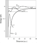
Figure 2: Probability amplitudes $\phi_{n}(z)$ and energies $\varepsilon_{n}$ of image-potential-induced bound states ($n=1,2,3$) outside an infinitely repulsive solid surface occupying the $z<0$ space (shaded area). The thick solid line represents the classical image potential of Eq. (43).

Image states are quantum states trapped in the long-range image-potential well outside a solid surface that presents a band gap near the vacuum level. In the case of a metal that occupies the half-space $z<0$, the asymptotic form of the potential experienced by an electron in the half space $z>0$ is the classical image potential

$$V(z)=-{1\over 4z}.$$ (43)

If one assumes (i) translational invariance in the plane of the surface and (ii) that due to the presence of a wide band gap at $z<0$ the solid surface is infinitely repulsive, i.e., $V(z)\to\infty$ at $z<0$ note1 , then one easily finds that the solutions of the corresponding one-particle Schrödinger equation represent a Rydberg-like series of image-potential induced bound states (see Fig. 2) of the form:

$$\psi_{{\bf k},n}({\bf r})={1\over\sqrt{A}}\,\phi_{n}(z)\,{\rm e}^{i{\bf k}\cdot{\bf r}_{\parallel}},$$ (44)

with energies

$$E_{{\bf k},n}=\varepsilon_{n}+{\bf k}^{2}/2,$$ (45)

where

$$\phi_{n}(z)\sim z\,\phi_{n}^{\rm hydrogen}(z/4),\,\,n=1,2,...$$ (46)

and

$$\varepsilon_{n}=-{1\over 32n^{2}},\,\,n=1,2,...,$$ (47)

$\phi_{n}^{\rm hydrogen}(z)$ representing the well-known wave functions of all possible $s$-like ($l=0$) bound states of the hydrogen atom. Here, ${\bf r}_{\parallel}$ and ${\bf k}$ represent the position and the wavevector in the $xy$ surface plane.

Inside the solid.

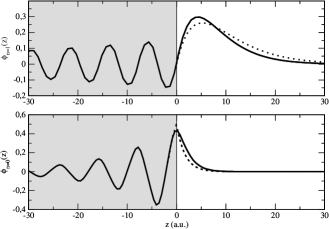
Figure 3: Probability amplitudes $\phi_{n}(z)$ of (a) Shockley ($n=0$) and (b) image ($n=1$) states on Cu(111). The dotted lines represent the results one obtains by matching at $z=0$ the wave function of Eqs. (48) and (49) to a mere exponential (for the Shockley state) or to the hydrogenic form of Eq. (46) with $n=1$ (for the $n=1$ image state). The solid lines represent the results one obtains by solving a 1D Schrödinger equation with the model potential of Chulkov et al. chulkov1 .

In the interior of the solid ($z<0$), both image and Shockley surface states can be described within a two-band approximation to the nearly-free-electron (NFE) band structure of the solid ashcroft . Assuming translational invariance in the plane of the surface and for a gap that is opened by potential Fourier components corresponding to reciprocal lattice vectors that are normal to the surface, surface-state wave functions within the crystal band gap take the form

$$\phi(z<0)\approx{\rm e}^{\Delta}\,\cos(Gz+\delta).$$ (48)

Here, $G$ represents the limit of the Brillouin zone in the direction normal to the surface, and

$$\Delta={1\over G}\sqrt{{1\over 4}V_{g}^{2}-\bar{\varepsilon}^{2}},$$ (49)

where $V_{g}$ and $\bar{\varepsilon}$ denote the energy gap and the surface-state energy with respect to the mid gap, respectively, and $\delta$ represents a phase shift which in the presence of a Shockley-inverted band gap forst varies from $-\pi/2$ for a surface-state energy $\varepsilon$ at the bottom of the gap to 0 for a surface-state energy at the top of the gap. Matching at $z=0$ to a wave function of the hydrogenic-like form of Eq. (46) (in the case of image states) or to a mere exponential (in the case of Shockley states) osma , one finds the wave functions $\phi_{n}(z)$ plotted by dotted lines in Fig. 3 for Cu(111).

III.3.2 One-dimensional model potentials

Still assuming translational invariance in two directions, i.e., assuming that the charge density and one-electron potential are constant in the plane of the surface, Chulkov et al. chulkov1 devised a simplified model that allows for realistic calculations while retaining at the same time the essential physics of electron and hole dynamics at solid surfaces. In the bulk region, this one-dimensional (1D) model potential is described by a cosine function which opens the energy gap on the surface of interest, the position and amplitude of this function being chosen to reproduce the energy gap observed experimentally and/or obtained from first-principles calculations at the $\bar{\Gamma}$ point. At the solid-vacuum interface, it is represented by a smooth cosine-like function that reproduces the experimental energy of the Shockley surface state. Finally, in the vacuum region this 1D potential merges into the long-range classical image potential of the form of Eq. (43) in such a way that the experimental binding energy of the first image state is reproduced. This model potential has been constructuted for several metal surfaces chulkov2 , and has been used widely for the investigation of electron and hole dynamics in a variety of situations.

The $n=0$ and $n=1$ eigenfunctions of a single-particle 1D hamiltonian that includes the model potential of Chulkov et al. for Cu(111) are plotted in Fig. 3 by solid lines, together with the NFE Shockley ($n=0$) and first image-state ($n=1$) wave functions described in the preceding section. In the bulk region, these wave functions coincide with the approximate NFE wave functions (represented in Fig. 3 by dotted lines); however, in the vacuum region the $n=1$ hydrogenic-like wave function of Eq. (46) appears to be too little localized near the surface. The $n=1$ eigenfunction of Chulkov’s 1D hamiltonian for Cu(100) chulkov0 was found to reproduce accurately the average probability density derived for that image state by Hulbert et al. hulbert from a first-principles calculation.

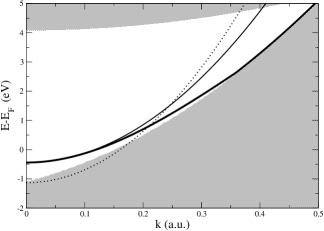
Figure 4: Dispersion of the Cu(111) Shockley surface state (thick solid line), as obtained from 3D ab initio calculations maia1 . Shaded areas represent areas outside the band gap, where bulk states exist. The thin solid and dotted lines represent approximate energy dispersions of the Shockley surface state and the bottom of the projected band gap, respectively, as obtained from an equation of the form of Eq. (45) with the Cu(111) $\bar{\Gamma}$-point Shockley-state energy (with respect to the Fermi level) $\varepsilon=-0.44\,{\rm eV}$ and the effective mass $m=0.42$ (thin solid line), and with the Cu(111) $\bar{\Gamma}$-point bottom-of-the-gap energy (with respect to the Fermi level) $\varepsilon=-1.09\,{\rm eV}$ and the effective mass $m=0.22$ (thin dotted line).

The assumption that the charge density and one-electron potential are constant in the plane of the surface is valid for the description of image states, since their wave functions lie mainly at the vacuum side of the surface and the electrons move, therefore, in a region with little potential variation parallel to the surface. Shockley and bulk states, however, do suffer a significant potential variation in the plane of the surface. In order to account approximately for this variation, the original 1D model potential of Chulkov et al. chulkov1 , which had been introduced to describe the projected band structure at the $\bar{\Gamma}$ point, was modified along with the introduction in Eq. (45) of a realistic effective mass for the dispersion curve of both bulk and surface states osma . Within this model, however, all Shockley states have the same effective mass, so the projected band structure is still inaccurate, especially at energies above the Fermi level, as shown in Fig. 4 for Cu(111).

As an alternative to the 1D model potential of Chulkov et al. chulkov1 , Vergniory et al. maia1 introduced a ${\bf k}$-dependent 1D potential that is constructed to reproduce the actual bulk energy bands and surface-state energy dispersion obtained from 3D first-principles calculations, thereby allowing for a realistic description of the electronic orbitals beyond the $\bar{\Gamma}$ point:

$$V_{k}(z)=\cases{U_{k}+2V_{k}\cos(2\pi z/a_{s}),&$z<z_{k}$\cr\cr\Phi&$z>z_{k}$.}$$ (50)

Here, $U_{k}$ and $V_{k}$ are fitted to the bulk energy bands, $a_{s}$ represents the interlayer spacing, $\Phi$ is the experimentally determined work function, and the matching plane $z_{k}$ is chosen to give the correct surface-state dispersion.

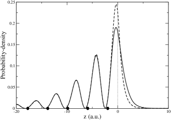
Figure 5: Probability-density $|\phi(z)|^{2}$ of the Shockley surface state at the center of the surface Brillouin zone ($\bar{\Gamma}$ point) of Cu(111), as obtained with the use of two different 1D model potentials: (i) the model potential of Chulkov et al. chulkov1 , which includes the image tail outside the surface but fails to reproduce the actual band structure beyond the $\bar{\Gamma}$ point (solid line), and (ii) the model potential of Eq. (50), which does not include the image tail outside the surface but is constructed to reproduce the actual bulk energy bands and surface-state energy dispersion beyond the $\bar{\Gamma}$ point (dashed line). Full circles represent the atomic positions of Cu in the (111) direction. The geometrical (jellium) electronic edge ($z=0$) has been chosen to be located half an interlayer spacing beyond the last atomic layer.

The abrupt 1D step model potential of Eq. (50), which does not account for the image tail outside the surface, could not possibly be used to describe image states. However, it has proved to be accurate for the description of Shockley surface states, which are known to be rather insensitive to the actual shape of the potential far outside the surface; indeed, the model potential of Eq. (50) is found to yield a surface-state probability density $|\phi(z)|^{2}$ at the band edge ($\bar{\Gamma}$ point, i.e., ${\bf k}=0$) of the Shockley surface-state band of Cu(111) that is in reasonably good agreement with the more realistic surface-state probability density obtained at $\bar{\Gamma}$ from the 1D model potential of Chulkov et al. chulkov1 , as shown in Fig. 5. Both probability densities coincide within the bulk, although the probability density obtained from the step model potential of Eq. (50) appears to be slightly more localized near the surface, as expected. For the overlap integral one finds $<\phi_{1}|\phi_{2}>=0.99$, $\phi_{1}$ and $\phi_{2}$ being the Shockley probability amplitudes leading to the probability densities represented in Fig. 5 by solid and dashed lines, respectively.

III.4 Screened interaction

The retarded counterpart of the density-response function entering Eq. (12), which in the framework of TDDFT can be obtained rigorously by solving the intergral Eq. (15), yields, within linear-response theory, the electron density $\delta n({\bf r},\omega)$ induced in a many-electron system by a frequency-dependent external potential $\phi^{ext}({\bf r},\omega)$:

$$\delta n({\bf r},\omega)=\int{\rm d}{\bf r}^{\prime}\,\chi({\bf r},{\bf r^{\prime}};\omega)\,\phi^{ext}({\bf r^{\prime}},\omega).$$ (51)

Hence, the retarded counterpart of the screened interaction $W({\bf r},{\bf r}^{\prime};\omega)$ of Eq. (12) yields, within linear-response theory, the total potential $\phi({\bf r},\omega)$ of a unit test charge at point ${\bf r}$ in the presence of an external test charge of density $n^{ext}({\bf r},\omega)$:

$$\phi({\bf r},\omega)=\int d{\bf r}^{\prime}\,W({\bf r},{\bf r}^{\prime};\omega)\,n^{ext}({\bf r}^{\prime},\omega),$$ (52)

which can also be expressed as follows

$$\phi({\bf r},\omega)=\int d{\bf r}^{\prime}\,\epsilon^{-1}({\bf r},{\bf r}^{\prime};\omega)\ \phi^{ext}({\bf r},\omega),$$ (53)

with

$$\epsilon^{-1}({\bf r},{\bf r}^{\prime};\omega)=\delta({\bf r}-{\bf r}^{\prime})+\int{\rm d}{\bf r}^{\prime\prime}\,v({\bf r}-{\bf r}^{\prime\prime})\,\chi({\bf r}^{\prime\prime},{\bf r}^{\prime};\omega).$$ (54)

This is the so-called inverse dielectric function of the many-electron system, whose poles dictate the occurrence of collective electronic excitations.

III.4.1 Classical model

In a classical model consisting of a semiinfinite solid at $z<0$ characterized by a local (frequency-dependent) dielectric function $\epsilon(\omega)$ separated by a planar surface from a semiinfinite vacuum at $z>0$, the total potential $\phi({\bf r},\omega)$ at each medium is a solution of Poisson’s equation

$$\nabla^{2}\phi({\bf r},\omega)=-{4\pi\over\epsilon_{i}(\omega)}\,n^{ext}({\bf r},\omega),$$ (55)

$\epsilon_{i}$ being $\epsilon(\omega)$ or $1$ depending on whether the point ${\bf r}$ is located in the solid or in the vacuum, respectively. Hence, the screened interaction $W({\bf r},{\bf r}^{\prime};\omega)$ entering Eq. (52) is a solution of the following equation:

$$\nabla^{2}W({\bf r},{\bf r}^{\prime};\omega)=-{4\pi\over\epsilon_{i}(\omega)}\,\delta({\bf r}-{\bf r}^{\prime}).$$ (56)

Imposing boundary conditions of continuity of the potential and the normal component of the displacement vector at the interface, one finds

$$W({\bf r},{\bf r}^{\prime};\omega)=\int d{\bf q}\,{\rm e}^{i{\bf q}\cdot({\bf r}_{\parallel}-{\bf r}_{\parallel}^{\prime})}\,W(z,z^{\prime};q,\omega),$$ (57)

where

$$W(z,z^{\prime};q,\omega)={2\pi\over q}\cases{\left[{\rm e}^{-q|z-z^{\prime}|}+g(\omega)\,{\rm e}^{-q(|z|+z^{\prime}|)}\right]/\epsilon(\omega),&$z<0,z^{\prime}<0$,\cr\cr 2\,g(\omega)\,{\rm e}^{-qz-z^{\prime}|}/\left[\epsilon(\omega)-1\right],&$z^{<}<0,z^{>}>0$,\cr\cr{\rm e}^{-q|z-z^{\prime}|}-g(\omega)\,{\rm e}^{-q(|z|+|z^{\prime}|)},&$z>0,z^{\prime}>0$,}$$ (58)

$z^{<}$ ($z^{>}$) being the smallest (largest) of $z$ and $z^{\prime}$, and $g$ being the classical surface-response function:

$$g(\omega)={\epsilon(\omega)-1\over\epsilon(\omega)+1}.$$ (59)

An inspection of Eqs. (58) and (59) shows that the screened interaction $W(z,z^{\prime};q,\omega)$ has poles at the classical bulk- and surface-plasmon conditions dictated by $\epsilon(\omega)=0$ and by $\epsilon(\omega)+1=0$, respectively plasmons . Since e-e inelastic linewidths of Shockley and image states are typically dominated by the excitation of electron-hole (e-h) pairs and not by the excitation of plasmons (whose energies are typically too large) notearan , the classical screened interaction of Eq. (58) (which obviously does not account for the excitation of e-h pairs) is of no use in this context.

III.4.2 Specular-reflection model (SRM)

A simple scheme that gives account of the excitation of e-h pairs, and has the virtue of expressing the screened interaction $W(z,z^{\prime};q,\omega)$ in terms of the dielectric function $\epsilon(q,\omega)$ of a homogeneous electron gas representing the bulk material, is the so-called specular-reflection model reported independently by Wagner wagner and by Ritchie and Marusak marusak . In this model, the semi-infinite solid is described by an electron gas in which all electrons are considered to be specularly reflected at the surface, thereby the electron density vanishing outside. One finds:

$$W(z,z^{\prime};q,\omega)={2\pi\over q}\cases{\epsilon_{s}(z-z^{\prime})+\epsilon_{s}(z+z^{\prime})-2\,g(q,\omega)\,\displaystyle{\epsilon_{s}(z)\,\epsilon_{s}(z^{\prime})\over 1-\epsilon_{s}^{0}},&$z<0,z^{\prime}<0$,\cr\cr 2\,g(q,\omega)\,\displaystyle{\epsilon_{s}(z^{<})\over 1-\epsilon_{s}^{0}}\,{\rm e}^{-qz^{>}},&$z^{<}<0,z^{>}>0$,\cr\cr{\rm e}^{-q|z-z^{\prime}|}-g(q,\omega)\,{\rm e}^{-q(z+z^{\prime})},&$z>0,z^{\prime}>0$,}$$ (60)

where the surface response function is now given by the following expression:

$$g(q,\omega)={1-\epsilon_{s}^{0}(q,\omega)\over 1+\epsilon_{s}^{0}(q,\omega)},$$ (61)

with

$$\epsilon_{s}(z;q,\omega)={q\over\pi}\int_{-\infty}^{+\infty}{dq_{z}\over Q^{2}}\,{\rm e}^{iq_{z}z}\epsilon^{-1}(Q,\omega),$$ (62)

$$\epsilon_{s}^{0}(q,\omega)=\epsilon_{s}(z=0;q,\omega),$$ (63)

and $Q=\sqrt{q^{2}+q_{z}^{2}}$. If the $Q$-dependence of the actual $\epsilon(Q,\omega)$ dielectric function of a homogeneous electron gas is ignored, the SRM screened interaction of Eq. (60) reduces to the classical screened interaction of Eq. (58).

The inverse dielectric function $\epsilon^{-1}(Q,\omega)$ entering Eq. (62) represents the 3D Fourier transform of the inverse dielectric function $\epsilon^{-1}({\bf r},{\bf r}^{\prime},\omega)$ of a homogeneous electron gas. From Eq. (54), one finds:

$$\epsilon^{-1}(Q,\omega)=1+v_{Q}\,\chi(Q,\omega),$$ (64)

where $\chi(Q,\omega)$ represents the 3D Fourier transform of the density-response function $\chi({\bf r},{\bf r}^{\prime};\omega)$, and $v_{Q}$ is the 3D Fourier transform of the bare Coulomb interaction $v({\bf r},{\bf r}^{\prime})$: $v_{Q}=4\pi/Q^{2}$.

In the framework of TDDFT, one uses Eq. (15) to find

$$\chi(Q,\omega)=\chi^{0}(Q,\omega)+\chi^{0}(Q,\omega)$$ (65)

(66)

$$\times\left\{v_{Q}+f^{xc}(n_{0};Q,\omega)\right\}\ \chi(Q,\omega),$$ (67)

with $\chi^{0}(Q,\omega)$ and $f^{xc}(n_{0};Q,\omega)$ being the 3D Fourier transforms of the noninteracting density-response function $\chi^{0}({\bf r},{\bf r}^{\prime};\omega)$ and the xc kernel $f^{xc}[n_{0}]({\bf r},{\bf r}^{\prime};\omega)$ of a homogeneous electron gas of density $n_{0}$. For a homogeneous electron gas, the eigenfunctions $\psi_{i}({\bf r})$ entering Eq. (18) are all plane waves; thus, the integrations can be carried out analytically to yield the well-known Lindhard function $\chi^{0}(Q,\omega)$ lindhard . If one sets the xc kernel $f^{xc}(n_{0};Q,\omega)$ equal to zero, the introduction of Eq. (65) into Eq. (64) yields the RPA dielectric function

$$\epsilon^{RPA}(Q,\omega)=1-v_{Q}\,\chi^{0}(Q,\omega),$$ (68)

which is easy to evaluate.

III.4.3 1D self-consistent scheme

For an accurate quantal description of the electronic excitations that occur in a semi-infinite solid, we need to consider the true self-consistent density-response function $\chi({\bf r},{\bf r}^{\prime};\omega)$ entering Eqs. (12) and (40).

Assuming translational invariance in the plane of the surface, one can still define the 2D Fourier transforms $W(z,z^{\prime};q,\omega)$ and $\tilde{W}(z,z^{\prime};q,\omega)$, which according to Eqs. (12) and (40) can be obtained as follows

$$W(z,z^{\prime};q,\omega)=v(z,z^{\prime};q)+\int dz_{1}\int dz_{2}\,v(z,z_{1};q)$$ (69)

(70)

$$\times\chi(z_{1},z_{2};q,\omega)\,v(z_{2},z^{\prime};q),$$ (71)

and

$$\tilde{W}(z,z^{\prime};q,\omega)=v(z,z^{\prime};q)+\int{\rm d}z_{1}\int{\rm d}z_{2}\,\left\{v(z,z_{1};q)\right.$$ (72)

(73)

$$+\left.f^{xc}[n_{0}](z,z_{1};q,\omega)\right\}\,\chi(z_{1},z_{2};q,\omega)\,v(z_{2},z^{\prime},q),$$ (74)

where $v(z,z^{\prime};q)$ is the 2D Fourier transform of the bare Coulomb interaction $v({\bf r},{\bf r}^{\prime})$:

$$v(z,z^{\prime};q)={2\pi\over q}\,{\rm e}^{-q|z-z^{\prime}|},$$ (75)

$f^{xc}[n](z,z^{\prime};q,\omega)$ is the 2D Fourier transform of the xc kernel $f^{xc}[n]({\bf r},{\bf r}^{\prime};\omega)$, and $\chi(z,z^{\prime};q,\omega)$ denotes the 2D Fourier transform of the interacting density-response function $\chi({\bf r},{\bf r}^{\prime};\omega)$. In the framework of TDDFT, one uses Eq. (15) to find:

$$\chi(z,z^{\prime};q,\omega)=\chi^{0}(z,z^{\prime};q,\omega)+\int dz_{1}\int dz_{2}\,\chi^{0}(z,z_{1};q,\omega)$$ (76)

(77)

$$\times\left\{v(z_{1},z_{2};q)+f^{xc}[n_{0}](z_{1},z_{2};q,\omega)\right\}\chi(z_{2},z^{\prime};q,\omega),$$ (78)

where $\chi^{0}(z,z^{\prime};q,\omega)$ denotes the 2D Fourier transform of the noninteracting density-response function $\chi^{0}({\bf r},{\bf r}^{\prime};\omega)$. Using Eq. (18), and noting that the single-particle orbitals $\psi_{i}({\bf r})$ now take the form

$$\psi_{{\bf k},i}({\bf r})=\phi_{i}(z)\,{\rm e}^{i{\bf k}\cdot{\bf r}_{\parallel}},$$ (79)

one finds:

$$\chi^{0}(z,z^{\prime};q,\omega)={2\over A}\mathrel{\mathop{\sum}\limits_{i,j}}\phi_{i}(z)\phi_{j}^{*}(z)\phi_{j}(z^{\prime})\phi_{i}^{*}(z^{\prime})$$ (80)

(81)

$$\times\mathop{\sum}\limits_{{\bf k}}\frac{f_{{\bf k},i}-f_{{\bf k}+{\bf q},j}}{E_{{\bf k},i}-E_{{\bf k}+{\bf q},j}+\omega+i\eta},$$ (82)

where $f_{{\bf k},i}$ are Fermi-Dirac occupation factors [which at zero temperature take the form $f_{{\bf k},i}=\Theta(\varepsilon_{F}-E_{{\bf k},i})$], and

$$E_{{\bf k},i}=\varepsilon_{i}+{k^{2}\over 2},$$ (83)

the single-particle orbitals $\phi_{i}(z)$ and energies $\varepsilon_{i}$ now being the eigenfunctions and eigenenergies of a 1D Kohn-Sham hamiltonian. In order to account for the actual band structure of $sp$ electrons near the surface of simple and noble metals, $\phi_{i}(z)$ and $\varepsilon_{i}$ have been succesfully taken to be the solutions of the 1D single-particle Schrödinger equation of Chulkov et al. chulkov1 described in the previous section.

III.4.4 Asymptotics

For $z$ and $z^{\prime}$ coordinates that are far from the surface into the vacuum, where the electron density vanishes, Eq. (69) takes the form notesrm

$$W(z,z^{\prime};q,\omega)=v(z,z^{\prime};q)-{2\pi\over q}\,{\rm e}^{-q(z+z^{\prime})}\,g(q,\omega),$$ (84)

with the surface-response function $g(q,\omega)$ now being given by the general expression liebsch0 :

$$g(q,\omega)=-{2\pi\over q}\,\int dz_{1}\int dz_{2}\,{\rm e}^{q(z_{1}+z_{2})}\,\chi(z_{1},z_{2};q,\omega).$$ (85)

Persson and Anderson pa and Persson and Zaremba pz investigated the structure of the so-called surface loss function ${\rm Im}g(q,\omega)$ for small $q$ and $\omega$. Persson and Zaremba found the following approximate result pz :

$${\rm Im}\,g=({\rm Im}\,g)_{surf}+({\rm Im}\,g)_{bulk}+({\rm Im}\,g)_{int},$$ (86)

where $({\rm Im}\,g)_{surf}$ and $({\rm Im}\,g)_{bulk}$ represent contributions from surface and bulk excitation of e-h pairs, and $({\rm Im}\,g)_{int}$ represents the contribution to the surface loss function coming from the interference between the bulk and surface excitations:

$$({\rm Im}\,g)_{surf}=2\xi{q\over k_{F}}{\omega\over\omega_{p}},$$ (87)

$$({\rm Im}\,g)_{bulk}={1\over 2}m_{opt}^{2}\left({\omega\over\omega_{p}}\right)^{2}\eta^{3}G(\eta),$$ (88)

and

$$({\rm Im}\,g)_{int}=-{8\over\pi^{2}}{m_{opt}\over k_{F}}\left({\omega\over\omega_{p}}\right)^{2}\eta{h\over 1+\eta^{2}},$$ (89)

with $\eta=\omega/(qk_{F})$ and

$$G(\eta)=8\cases{1,&for $\eta<1$,\cr\cr 1-(1+{1\over 2}\eta^{-2})(1-\eta^{-2})^{1/2},&for $\eta>1$.\cr\cr}$$ (90)

Here, $k_{F}$ and $\omega_{p}$ represent the Fermi momentum and the plasmon frequency, respectively: $k_{F}^{3}=3\pi^{2}\bar{n}_{0}$ and $\omega_{p}^{2}=4\pi\bar{n}_{0}$, $\bar{n}_{0}$ being the mean electron density. The values of $\xi$, $m_{opt}$, and $h$ are given in Ref. pz . The surface contribution of Eq. (87) had already been reported in Ref. pa , the bulk contribution of Eq. (88) differs from that used in Ref. pa by the factor of the optical mass and a factor of $1\over 2$ which had been missed previously, and the contribution $({\rm Im}\,g)_{int}$ had been neglected in Ref. pa .

III.4.5 The xc kernel $f^{xc}[n](z,z^{\prime};q,\omega)$

Several approximations can be used to evaluate the unknown xc kernel $f^{xc}[n_{0}](z,z^{\prime};q,\omega)$ entering Eqs. (72) and (76).

Random-phase approximation (RPA).

Nowadays one usually refers to the RPA as the result of simply setting the xc kernel $f^{xc}[n](z,z^{\prime};q,\omega)$ equal to zero: $f^{xc}[n](z,z^{\prime};q,\omega)=0$, but still using in Eqs. (79) and (83) single-particle Kohn-Sham states and energies $\phi_{i}(z)$ and $\varepsilon_{i}$ that go beyond the Hartree approximation.

Adiabatic local-density approximation (ALDA).

If one assumes that dynamic electron-density fluctuations are slowly varying in all directions, the xc kernel $f^{xc}[n](z,z^{\prime};q,\omega)$ is easily found to be given by the following expression liebsch0 :

$$f^{xc}[n](z,z^{\prime};q,\omega)=\bar{f}^{xc}(n=n(z);Q=0,\omega=0)\,\delta(z-z^{\prime}).$$ (91)

Here, $\bar{f}^{xc}(n=n(z);Q,\omega)$ is the 3D Fourier transform of the xc kernel of a homogeneous electron gas of density $n$ equal to the local density $n(z)$, which in the limit as $Q\to 0$ and $\omega\to 0$ is known to be the second derivative of the xc energy per particle $\varepsilon_{xc}(n)$. One typically uses parametrizations pw of the diffusion Monte Carlo (DMC) xc energy $\varepsilon_{xc}$ reported by Ceperley and Alder ca .

Adiabatic nonlocal approximation (ANLDA).

The investigation of short-range xc effects in solids has focused to a great extent onto the homogeneous electron gas constantin . Hence, assuming that the unperturbed density variation $\left[n(z)-n(z^{\prime})\right]$ is small within the short range of $f^{xc}[n](z,z^{\prime};q,\omega)$, one can adopt the following average adiabatic nonlocal approximation delsole3 ; lein ; pp :

$$f^{xc}[n](z,z^{\prime};q,\omega)=\bar{f}^{xc}(\left[n(z)+n(z^{\prime})\right]/2;z,z^{\prime};q,\omega=0),$$ (92)

where $\bar{f}^{xc}(n;z,z^{\prime};q,\omega)$ represents the 1D Fourier transform of the xc kernel $\bar{f}^{xc}(n;Q,\omega)$ of a homogeneous electron gas of density $n$. A parametrization of the accurate DMC calculations reported by Moroni et al. moroni for the static ($\omega=0$) $Q$-dependent nonlocal xc kernel $\bar{f}^{xc}(n;Q,\omega=0)$ that satisfies the well-known small and large-wavelength asymptotic behaviour was carried out by Corradini et al. (CDOP) corradini . An explicit expression for the 2D Fourier transform of the CDOP parametrization of $\bar{f}^{xc}(n;Q,\omega=0)$ was reported in Ref. pp :

$$\bar{f}^{xc}(n;z,z^{\prime};k)=-\frac{4\pi e^{2}C}{k_{F}^{2}}\delta(\tilde{z})-\frac{2\pi e^{2}B}{\sqrt{gk_{F}^{2}+k^{2}}}\,{\rm e}^{-\sqrt{gk_{F}^{2}+k^{2}}|\tilde{z}|}-\frac{2\alpha\sqrt{\pi/\beta}e^{2}}{k_{F}^{3}}\left[\frac{2\beta-k_{F}^{2}\tilde{z}^{2}}{4\beta^{2}}k_{F}^{2}+k^{2}\right]{\rm e}^{-\beta\left[k_{F}^{2}\tilde{z}^{2}/4\beta^{2}+k^{2}/k_{F}^{2}\right]},$$ (93)

where $C$, $B$, $g$, $\alpha$, and $\beta$ are dimensionless functions of the electron density (see Ref. corradini ), $k_{F}=(3\pi^{2}n)^{1/3}$, and $\tilde{z}=z-z^{\prime}$.

Calculations of the frequency dependence of the xc kernel of a homogeneous electron gas have been carried out mainly in the limit of long wavelengths v1 ; v2 ; v3 ; v4 ; v5 ; v6 , but work has also been done for finite wave vectors z1 ; z2 ; z3 ; z4 . Approximate expressions for the frequency-dependent xc kernel of inhomogeneous systems have been reported in Refs. petersilka ; burke ; delsole2 ; nazarov .

III.4.6 $d-$electron screening

The 1D self-consistent scheme described above has proved to be appropriate for the description of the screened interaction of $sp$ electrons in simple and noble metals. It has been argued, however, in the past that a realistic first-principles description of the electronic band structure is of key importance in the determination of the inelastic lifetime of bulk electronic states in the noble metals, due to the participation of $d$ electrons in the screening of e-e interactions campillo .

Following the scheme originally developed by Liebsch to describe the anomalous dispersion of surface plasmons in Ag liebsch1 , García-Lekue et al. aran accounted for the presence of occupied $d$-bands in the noble metals by assuming that $sp$ valence electrons are embedded in a polarizable background at $z\leq z_{0}$ characterized by a local dielectric function $\epsilon_{d}(\omega)$. Within this model, the bare Coulomb interaction $v(z,z^{\prime};q)$ entering Eq. (76) is replaced by a modified ($d$-screened) Coulomb interaction $v^{\prime}(z,z^{\prime};q,\omega)$ whose 2D Fourier transform yields catalina

$$v^{\prime}(z,z^{\prime};q,\omega) = \frac{2\pi}{q\,\epsilon_{d}(z^{\prime},\omega)}\,[{\rm e}^{-q\,|z-z^{\prime}|}+{\rm sgn}(z_{d}-z^{\prime})$$ (94)

$$\times \sigma_{d}(\omega)\,{\rm e}^{-q|z-z_{d}|}{\rm e}^{-q|z_{d}-z^{\prime}|}],$$

where

$$\epsilon_{d}(z,\omega)=\cases{\epsilon_{d}(\omega),&$z\leq z_{d}$\cr\cr 1,&$z>z_{d}$}$$ (95)

and

$$\sigma_{d}={\epsilon_{d}(\omega)-1\over\epsilon_{d}(\omega)+1}.$$ (96)

The first term in Eq. (94) is simply the 2D Fourier transform of the bare Coulomb interaction [see Eq. (75)], but now screened by the polarization charges induced within the polarizable background. The second term stems from polarization charges at the boundary of the medium.

III.4.7 Periodic surface

For a real periodic surface, one may introduce the following Fourier expansion of the screened interaction:

$$W({\bf r},{\bf r}^{\prime};\omega) = {1\over A}\sum_{\bf q}^{SBZ}\sum_{{\bf g},{\bf g}^{\prime}}{\rm e}^{i({\bf q}+{\bf g})\cdot{\bf r}_{\parallel}}{\rm e}^{-i({\bf q}+{\bf g}^{\prime})\cdot{\bf r}_{\parallel}^{\prime}}$$ (97)

$$\times W_{{\bf g},{\bf g}^{\prime}}(z,z^{\prime};{\bf q},\omega),$$ (99)

where ${\bf q}$ is a 2D wave vector in the surface Brillouin zone (SBZ), and ${\bf g}$ and ${\bf g}^{\prime}$ denote 2D reciprocal-lattice vectors. According to Eq. (12), the 2D Fourier coefficients $W_{{\bf g},{\bf g}^{\prime}}(z,z^{\prime};{\bf q},\omega)$ are given by the following expression:

$$W_{{\bf g},{\bf g}^{\prime}}(z,z^{\prime};{\bf q},\omega)=v_{\bf g}(z,z^{\prime};{\bf q})\,\delta_{{\bf g},{\bf g}^{\prime}}+\int dz_{1}\int dz_{2}$$ (100)

(101)

$$\times v_{\bf g}(z,z_{1};{\bf q})\,\chi_{{\bf g},{\bf g}^{\prime}}(z_{1},z_{2};{\bf q},\omega)\,v_{{\bf g}^{\prime}}(z_{2},z^{\prime};{\bf q}),$$ (102)

where $v_{\bf g}(z,z^{\prime};{\bf q})$ denote the 2D Fourier coefficients of the bare Coulomb interaction $v({\bf r},{\bf r}^{\prime})$:

$$v_{\bf g}(z,z^{\prime};{\bf q})={2\pi\over|{\bf q}+{\bf g}|}\,{\rm e}^{-|{\bf q}+{\bf g}|\,|z-z^{\prime}|},$$ (103)

and $\chi_{{\bf g},{\bf g}^{\prime}}(z,z^{\prime};{\bf q},\omega)$ are the Fourier coefficients of the interacting density-response function $\chi({\bf r},{\bf r}^{\prime};\omega)$. In the framework of TDDFT, one uses Eq. (15) to find:

$$\chi_{{\bf g},{\bf g}^{\prime}}(z,z^{\prime};{\bf q},\omega)=\chi_{{\bf g},{\bf g}^{\prime}}^{0}(z,z^{\prime};{\bf q},\omega)+\int dz_{1}\int dz_{2}$$ (104)

(105)

$$\times\chi_{{\bf g},{\bf g}^{\prime}}^{0}(z,z_{1};{\bf q},\omega)\,\times\left[v_{{\bf g}_{1}}(z_{1},z_{2};{\bf q})\,\delta_{{\bf g}_{1},{\bf g}_{2}}\right.$$ (106)

(107)

$$\left.+f_{{\bf g}_{1},{\bf g}_{2}}^{xc}[n_{0}](z_{1},z_{2};{\bf q},\omega)\right]\chi_{{\bf g}_{2},{\bf g}^{\prime}}(z_{2},z^{\prime};{\bf q},\omega),$$ (108)

where $\chi_{{\bf g},{\bf g}^{\prime}}^{0}(z,z^{\prime};{\bf q},\omega)$ and $f_{{\bf g},{\bf g}^{\prime}}^{xc}[n_{0}](z,z^{\prime};{\bf q},\omega)$ denote the Fourier coefficients of the noninteracting density-response function $\chi^{0}({\bf r},{\bf r}^{\prime};\omega)$ and the xc kernel $f^{xc}[n_{0}]({\bf r},{\bf r}^{\prime};\omega)$, respectively. Using Eq. (18), one finds:

$$\chi_{{\bf g},{\bf g}^{\prime}}^{0}(z,z^{\prime};{\bf q},\omega)=\frac{2}{A}\,\sum_{\bf k}^{\rm SBZ}\sum_{n,n^{\prime}}\frac{f_{{\bf k},n}-f_{{\bf k}+{\bf q},n^{\prime}}}{\varepsilon_{{\bf k},n}-\varepsilon_{{\bf k}+{\bf q},n^{\prime}}+\omega+{i}\eta}$$ (109)

(110)

$$\times\left\langle\phi_{{\bf k},n}(z)|e^{-{i}({\bf q}+{\bf g})\cdot{\bf r}_{\parallel}}|\phi_{{\bf k}+{\bf q},n^{\prime}}(z^{\prime})\right\rangle$$ (111)

(112)

$$\times\left\langle\phi_{{\bf k}+{\bf q},n^{\prime}}(z^{\prime})|e^{{i}({\bf q}+{\bf g}^{\prime})\cdot{\bf r}_{\parallel}}|\phi_{{\bf k},n}(z)\right\rangle,$$ (113)

the single-particle orbitals $\phi_{{\bf k},n}({\bf r})$ and energies $\varepsilon_{{\bf k},n}$ being the eigenfunctions and eigenvalues of a 3D Kohn-Sham Hamiltonian with an effective potential that is periodic in the plane of the surface.

IV Results and discussion

IV.1 Image states

The first quantitative evaluation of image-state lifetimes was reported in Ref. sols . This calculation was carried out from Eqs. (4) and (8), with (i) the hydrogenic-like image-state wave function $\phi_{i}(z)$ of Eq. (46) with $n=1$ and no penetration into the solid, (ii) the bulk final state wave functions $\phi_{f}(z)$ obtained with the use of a step model potential, and (iii) two simplified models for the screened interaction: the SRM of Eq. (60) with the RPA for the bulk dielectric function, and the surface response function reported by Persson and Anderson pa . In subsequent calculations the penetration of the image-state wave function into the crystal was allowed deandres , and the role that the unoccupied part of the narrow Shockley surface state on the (111) surfaces of Cu and Ni plays in the decay of the $n=1$ image state on these surfaces was investigated by Gao and Lundqvist gao . In this work, the image-state wave functions were also approximated by hydrogenic-like wave functions of the form of Eq. (46) with no penetration into the solid, a simplified parametrized form was used for the Shockley surface-state wave function, and screening effects were neglected altogether. A $G^{0}W^{0}$ calculation of the imaginary part of the electron self-energy near a jellium surface was also reported deisz , showing the key role that a full evaluation of this quantity may play in the description of surface-state lifetimes.

The first self-consistent many-body calculations of image-state lifetimes on noble and simple metals were reported by Chulkov et al. chulkov0 ; chulkov3 , and good agreement with the experimentally determined decay times hofer ; knoesel ; shumay was found. In these calculations, all wave functions and energies were obtained by solving a single-particle Schrödinger equation with the physically motivated 1D model potential of Ref. chulkov1 , and the electron self-energy was evaluated in the $G^{0}W^{0}$ approximation. The potential variation in the plane of the surface was considered later through the introduction of an effective mass osma , and self-consistent calculations of the key role that the partially occupied Shockley surface state plays in the decay of image states on Cu(111) were carried out osma . The inclusion of xc effects was investigated in the framework of the $GW\Gamma$ approximation, first with an adiabatic local-density description sarria and more recently with an adiabatic non-local description of the xc kernel maia2 .

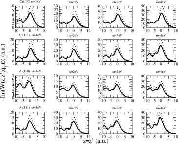
Figure 6: Imaginary part of the screened interaction $W(z,z^{\prime};q,\omega)$ and the effective screened interaction $\tilde{W}(z,z^{\prime};q,\omega)$, as a function of $z=z^{\prime}$ for a fixed value of $k$ ($q=0.5\,{\rm\AA}^{-1}$) and various values of $\omega$ ($\omega=1,2,3,4\,{\rm eV}$), in the vicinity of the (100) and (111) surfaces of Cu and Au. ANLDA calculations of ${\rm Im}\left[\tilde{W}(z,z^{\prime};q,\omega)\right]$ are represented by thick solid lines. RPA and ANLDA calculations of ${\rm Im}\left[W(z,z^{\prime};q,\omega)\right]$ are represented by thin solid and dotted lines, respectively. The RPA ${\rm Im}\left[W(z,z^{\prime};q,\omega)\right]$ and the ANLDA ${\rm Im}\left[W(z,z^{\prime};q,\omega)\right]$ are nearly indistinguishable, as a result of a cancellation between the xc effects due to the presence of (i) an xc hole associated with all electrons in the Fermi sea and (ii) an xc hole associated with the excited electron or hole.

The impact of xc effects on the imaginary part of the effective screened interaction of Eq. (72) in the vicinity of the (100) and (111) surfaces of Cu and Au is illustrated in Fig. 6, where ANLDA calculations of ${\rm Im}[\tilde{W}(z,z^{\prime};q,\omega)]$ (with full inclusion of xc effects) are compared to calculations of ${\rm Im}[W(z,z^{\prime};k,\omega)]$ with (ANLDA) and without (RPA) xc effects. Exchange-correlation effects included in the effective screened interaction have two sources. First, there is the reduction of the screening due to the presence of an xc hole associated with all electrons in the Fermi sea [see Eq. (76)], which is included in the calculations represented in Fig. 6 by thick solid lines and also in the calculations represented by dotted lines. Secondly, there is the reduction of the effective screened interaction itself due to the xc hole associated with the excited electron or hole [see Eq. (72)], which is only included in the calculations represented in Fig. 6 by thick solid lines. These contributions have opposite signs, thereby bringing the ANLDA ${\rm Im}[\tilde{W}(z,z^{\prime};k,\omega)]$ (thick solid lines) back to the RPA ${\rm Im}[W(z,z^{\prime};k,\omega)]$ (thin solid lines).

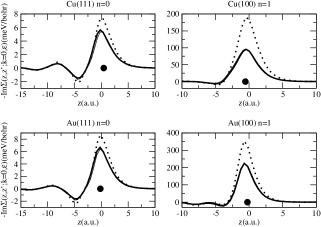
Figure 7: $G^{0}W^{0}$ ($G^{0}W$-RPA), $G^{0}W$, and $GW\Gamma$ calculations of the imaginary part of the $n=1$ image-state self-energy $\Sigma(z,z^{\prime};{\bf k}=0,\varepsilon_{\bf k})$, versus $z$, in the vicinity of the (100) surfaces of Cu and Au. The solid circle represents the value of $z^{\prime}$ in each case. $GW\Gamma$ calculations (as obtained with the use of our ANLDA xc kernel) are represented by thick solid lines. $G^{0}W$ (also using our ANLDA xc kernel) and $G^{0}W^{0}$ calculations are represented by dotted and thin solid lines, respectively. ALDA calculations, not plotted in this figure, are found to nearly concide with ANLDA calculations.

Figure 7 exhibits $G^{0}W^{0}$, $G^{0}W$, and $GW\Gamma$ calculations of the imaginary part of the ${\bf k}$-resolved $n=1$ image-state self-energy $\Sigma(z,z^{\prime};{\bf k}=0,\varepsilon_{\bf k})$, versus $z$, in the vicinity of the (100) surfaces of Cu and Au, with use (in the case of the $G^{0}W$ and $GW\Gamma$ approximations) of the adiabatic nonlocal xc kernel (ANLDA) described in Sec. III.4.5. This figure shows that as occurs in the case of the screened interaction xc effects partially compensate each other, leading to an overall effect of no more than 5% percent. We note that, as anticipated in Ref. maia2 for the case of Cu(111), although the ALDA leads to spurious results for the screened interaction our more realistic ANLDA kernel yields self-energies that esentially coincide with those obtained in the ALDA.

Table 2: Reciprocal lifetimes, in linewidth units (meV), of the $n=1$ image state (at $\bar{\Gamma}$, i.e., ${\bf k}=0$) on Cu(100), together with the most recent measurement reported in Ref. hofer2 . All the single-particle wave functions and energies entering Eqs. (4), (8), (30), and (36) have been chosen to be the eigenfunctions and eigenvalues of the 1D Hamiltonian of Chulkov et al. chulkov1 . Effective masses for all the single-particle energies entering Eqs. (8), (30), and (36) have been set equal to either the free-electron mass ($m_{f}=1$) or to realistic values ($m_{f}\neq 1$). Various models have been considered for the description of the electron self-energy, as obtained from (i) Eq. (8) with the screened interaction of Eq. (60) (SRM), of Eqs. (84)-(90) (PZ), and of Eqs. (69) and (76) with $f^{xc}[n_{0}](z,z^{\prime};q,\omega)$ set equal to zero ($G^{0}W^{0}$), (ii) Eq. (30) with the screened interaction of Eqs. (69) and (76) and the ANLDA xc kernel $f^{xc}[n_{0}](z,z^{\prime};q,\omega)$ ($G^{0}W$), and (iii) Eq. (36) with the effective screened interaction of Eqs. (72) and (76) and the ANLDA xc kernel $f^{xc}[n_{0}](z,z^{\prime};q,\omega)$ ($GW\Gamma$).

$m_{f}$	Self-energy	Bulk	Vacuum	Mix	Total	Exp.
=1	SRM	18	3	-4	17
=1	PZ		55		55
=1	$G^{0}W^{0}$	24	14	-16	22
$\neq 1$	$G^{0}W^{0}$	7	11.5	-1	17.5
$\neq 1$	$G^{0}W$				24.5
$\neq 1$	$GW\Gamma$	6.5	11.5	-1	17
						16

Table 3: As in Table 2, but for Cu(111) and together with the reciprocal lifetime experimentally determined for this surface at low temperature, $T=25\,{\rm K}$ knoesel .

$m_{f}$	Self-energy	Bulk	Vacuum	Mix	Total	Exp.
=1	SRM	46	12	-22	36
=1	PZ		57		57
=1	$G^{0}W^{0}$	44	47	-54	37
$\neq 1$	$G^{0}W^{0}$	32	34	-37	29
$\neq 1$	$G^{0}W$				43
$\neq 1$	$GW\Gamma$	30	35	-38	28
						30

Tables 2 and 3 exhibit the linewidth of the $n=1$ image state (at $\bar{\Gamma}$, i.e., ${\bf k}=0$) on the (100) and (111) surfaces of Cu, as obtained from Eq. (4) with (i) the image-state wave function of Chulkov et al. chulkov1 described in Sec. III.3.2 and (ii) various approximations for the self-energy: $SRM$, $PZ$, $G^{0}W^{0}$, $G^{0}W$, and $GW\Gamma$. Contributions to the linewidth are separated as follows

$$\Gamma_{ee}=\Gamma_{bulk}+\Gamma_{vac}+\Gamma_{mix},$$ (114)

where $\Gamma_{bulk}$, $\Gamma_{vac}$, and $\Gamma_{mix}$ represent bulk, vacuum, and mixed contributions, respectively, as obtained by confining the integrals in Eqs. (4) to either bulk ($z<0,z^{\prime}<0$), vacuum ($z>0,z^{\prime}>0$), or mixed ($z\geq 0,z^{\prime}\leq 0$ or $z\leq 0,z^{\prime}\geq 0$) coordinates.

First of all, we set all effective masses equal to the free-electron mass, and focus on the role that an accurate description of the screened interaction plays in the coupling of image states with the solid, by comparing to the results obtained (within the $G^{0}W^{0}$ approximation) with the use of the SRM screened interaction and (for the vacuum linewidth) the screened interaction of Persson and Zaremba (PZ). We note that simplified jellium models for the evaluation of the screened interaction yield unrealistic results for the image-state lifetime. Bulk contributions to the linewidth are approximately well described within the SRM, small differences resulting from an approximate description, within this model, of the so-called begrenzung or boundary-effect first described by Ritchie ritchie1 . However, as quantum-mechanical details of the surface are ignored within this model, it fails to describe both vacuum and mixed contributions to the decay rate. These quantum-mechanical details of the surface are approximately taken into account within the PZ approach, but the PZ model cannot account for the coupling of the image state with the crystal that occurs through the penetration of the image-state wave function into the solid. Discrepancies between vacuum contributions obtained in this model and in the more realistic full $G^{0}W^{0}$ approach appear as a result of the PZ model being accurate only for small ${\bf q}$ wave vectors and $\omega$ frequencies.

Now we account for the variation of the potential in the plane of the surface through the introduction of a realistic effective mass for all surface and bulk states. The effective masses of the $n=1$ image state on Cu(100) and Cu(111) are close to the free-electron mass ($m_{i}=1$). Nevertheless, the effective mass of the $n=0$ Shockley surface state of Cu(111) and the unoccupied bulk states in Cu(111) and Cu(100), which all contribute to the decay of the $n=1$ image state, considerably deviate from the free-electron mass; Tables 2 and 3 show that the impact of this deviation on the $n=1$ image-state lifetime is not neglegible.

As for the impact of short-range xc effects, which are fully incorporated in the framework of the $GW\Gamma$ approximation, Tables 2 and 3 show that the overall impact of these effects is small and $GW\Gamma$ reciprocal lifetimes are close to their $G^{0}W^{0}$ counterparts.

Table 4: $G^{0}W^{0}$, $G^{0}W$, and $GW\Gamma$ reciprocal lifetimes, in linewidth units (meV), of the $n=1$ image state (at $\bar{\Gamma}$, i.e., ${\bf k}=0$) on Au(100). In the case of the $G^{0}W$ and $GW\Gamma$ reciprocal lifetimes, both ALDA and ANLDA xc kernels have been considered.

xc kernel	$G^{0}W^{0}$	$G^{0}W$	$GW\Gamma$
	30
ALDA		42.5	31
ANLDA		43	31

ALDA and ANLDA $GW\Gamma$ calculations of the reciprocal lifetimes of the $n=1$ image state on Au(100), never reported before, are exhibited in Table 4. For comparison, this Table also shows $G^{0}W^{0}$ and $G^{0}W$ calculations, which in the case of the $G^{0}W$ have been obtained by considering (as within the $GW\Gamma$ approximation) both local (ALDA) and nonlocal (ANLDA) xc kernels. As occurs in the case of Cu maia2 , the results shown in Table 4 indicate that (i) a realistic adiabatic nonlocal description of xc effects yields reciprocal lifetimes of image states that esentially coincide with those obtained in the ALDA, and (ii) the overall effect of short-range exchange and correlation is small, thereby $GW\Gamma$ reciprocal lifetimes being close to their $G^{0}W^{0}$ counterparts.

Table 5: Linewidth (inverse lifetime) of image states, in meV. The lifetime in fs ($1\,{\rm fs}=10^{-15}s$) is obtained by noting that $\hbar=658\,{\rm meV}\,{\rm fs}$. The numbers in brackets represent the corresponding references. Electron-phonon linewidths are not included, since in the case of image states they are all expected to be below 1 meV eiguren3 .

	$G^{0}W^{0}$	$GW\Gamma$	Exp.
Li(110)	$37$ sarria
Cu(100)	$17.5$ sarria	$17$ maia2	$16.5\pm 2.5$ hofer ; shumay
			16 hofer2
Cu(111)	$29$ sarria	$28$ maia2	$30$ knoesel
			$29\pm 6$ weinelt
Ag(100)	12 aran		$12\pm 1$ shumay
Ag(111)	36 aran		$21\pm 9/5$ lingle
Au(100)	30 chulkovchem	31
Pd(111)	30 pd		$26\pm 5/3$ pd
Pt(111)	23 pt		$25\pm 10/5$ pt
Ni(100)	33 chulkovchem		$41\pm 19/10$ ni100
Ni(111)	44 chulkovchem		$94\pm 71/28$ ni111
Ru(1000)	47 echeap		59 ruexp

In Table 5, we compare self-consistent $G^{0}W^{0}$ and $GW\Gamma$ (as obtained with the ANLDA xc kernel) calculations (with full inclusion of realistic values of the effective mass of all bulk and surface states) with the existing TR-2PPE data for the $n=1$ image state at the $\bar{\Gamma}$ point (${\bf k}=0$) on various simple, noble, and transition single-crystal surfaces. This table shows that $G^{0}W^{0}$ and $GW\Gamma$ calculations are both in good agreement with TR-2PPE measurements except in the case of the (111) surfaces of the noble metal Ag and the transition metal Ni. The largest disagreement occurs in the case of Ni(111), where the $G^{0}W^{0}$ linewidth is smaller than the measured linewidth by approximately a factor of 2. This can be attributed to the necessity of a full ab initio description of the dynamical response of both $sp$ and $d$ electrons along the lines of Sec. III.4.7.

The role that occupied $d$ bands play in the dynamics of image states on silver surfaces was investigated in Ref. aran along the lines described in Sec. III.4.6. It was concluded that $d$ electrons do play an important role as a consequence of the reduction (in the presence of $d$ electrons) of the surface-plasmon energy that allows the opening of a new decay channel. No surface-plasmon decay channel is opened, however, in the case of the other noble-metal surafces (Cu and Au), since in the presence of $d$ electrons the Cu and Au surface-plasmon energy is still too large.

IV.2 Shockley states

$G^{0}W^{0}$ calculations of the e-e inelastic lifetimes of excited holes at the surface-state band edge of the (111) surfaces of the noble metals Cu, Ag, and Au were first reported in Refs. science and echeap within the 1D scheme of Chulkov et al. chulkov1 (see Sec. III.3.2), accounting for the potential variation in the plane of the surface through the introduction of a realistic effective mass for the dispersion curve of both bulk and surface states. Within this model, however, all Shockley states have the same effective mass and the projected band structure is still inaccurate, especially at energies above the Fermi level, as shown in Fig. 4 for Cu(111). As an alternative to the 1D model potential of Chulkov et al. chulkov1 , Vergniory et al. maia1 introduced the ${\bf k}$-dependent 1D potential of Eq. (50) that is constructed to reproduce the bulk energy bands and surface-state energy dispersion obtained from 3D first-principles calculations.

Table 6: $G^{0}W^{0}$, $G^{0}W$, and $GW\Gamma$ decay rates, in linewidth units (meV), of an excited hole at the band edge of the Shockley surface-state band of Cu(111) ($E_{i}=-0.44\,{\rm eV}$ and $k_{i}=0$). The $G^{0}W^{0}$ calculations have been performed either with the use of the ${\bf k}$-dependent 1D model potential of Eq. (50), as reported in Ref. maia1 , or with the use of the 1D scheme of Chulkov et al. chulkov1 , as reported in Refs. science and echeap . The $G^{0}W$ and $GW\Gamma$ calculations have been performed with the use of the 1D scheme of Chulkov et al. chulkov1 , as reported in Ref. maia2 . The experimental linewidth has been taken from the STM measurements reported in Ref. science . The total decay rate $\Gamma_{\rm total}$ includes the e-ph decay rate of 7 meV reported in Ref. eiguren2 . $\Gamma_{\rm inter}$ and $\Gamma_{\rm intra}$ represent interband and intraband contributions to the e-e decay rate $\Gamma_{\rm e-e}$; these contributions come from the decay of the excited hole trhough the coupling with bulk states (interband contribution) or thorugh the coupling, within the surface-state band itself, with surface states of different wave vector ${\bf k}$ parallel to the surface (intraband contribution).

	$\Gamma_{\rm inter}$	$\Gamma_{\rm intra}$	$\Gamma_{\rm e-e}$	$\Gamma_{\rm total}$
$G^{0}W^{0}$ maia1	10	9	19	26
$G^{0}W^{0}$ science ; echeap	6	19	25	32
$G^{0}W$ maia2			30.5	37.5
$GW\Gamma$ maia2			24.5	31.5
Experiment				24

Table 6 shows a comparison between the $G^{0}W^{0}$ calculations reported in Refs. science ; echeap and maia1 for the inelastic lifetime of an excited hole at the band edge of the Shockley surface-state band of Cu(111), as obtained from Eqs. (4) and (5) with the use of the 1D scheme of Chulkov et al. chulkov1 and with the ${\bf k}$-dependent 1D model potential of Eq. (50), respectively. The difference between the surface-state lifetime broadening of $25\,{\rm eV}$ reported in Refs. science and echeap and the more accurate lifetime broadening of $19\,{\rm eV}$ reported in Ref. maia1 is entirely due to a more accurate description in Ref. maia1 of (i) the projected band structure and (ii) the wave-vector dependence of the surface-state wave functions entering the evaluation of the self-energy. $G^{0}W$ and $GW\Gamma$ calculations were reported in Ref. maia2 , showing that as in the case of image states $GW\Gamma$ linewidths are only slightly lower than their $G^{0}W^{0}$ counterparts.

At this point, we note that the linewidths of the Cu(111) Shockley state at $\bar{\Gamma}$ based on the use of the two 1D models of Sec. III.3.2 to describe the initial surface-state wave function (at $\bar{\Gamma}$) agree within less than 1 meV. The linewidths also agree within less than 1 meV when the actual surface-state dispersion (thick solid line of Fig. 4) is replaced by the parabolic surface-state dispersion of the form dictated by the thin solid line of Fig. 4. However, if one replaces in the calculation of Ref. maia1 the wave-vector dependent surface-state orbitals obtained by solving a 1D Schrödinger equation with the potential of Eq. (50) by their less accurate counterparts used in Refs.  science and echeap , the lifetime broadening is increased considerably (from 19 to 25 meV), showing the important role that the actual coupling between initial and final states plays in the surface-state decay mechanism.

Table 7: $G^{0}W^{0}$, $G^{0}W$, and $GW\Gamma$ reciprocal lifetimes, in linewidth units (meV), of the $n=0$ Shockley state (at $\bar{\Gamma}$, i.e., ${\bf k}=0$) on Au(111). In the case of the $G^{0}W$ and $GW\Gamma$ reciprocal lifetimes, both ALDA and ANLDA xc kernels have been considered.

xc kernel	$G^{0}W^{0}$	$G^{0}W$	$GW\Gamma$
	29
ALDA		39.5	30
ANLDA		40	30

ALDA and ANLDA $GW\Gamma$ calculations of the reciprocal lifetimes of the Shockley surface state on Au(111), never reported before, are exhibited in Table 7. For comparison, this Table also shows $G^{0}W^{0}$ and $G^{0}W$ calculations, which in the case of the $G^{0}W$ have been obtained by considering (as within the $GW\Gamma$ approximation) both local (ALDA) and nonlocal (ANLDA) xc kernels. As occurs in the case of Cu maia2 , the results shown in Table 7 indicate that (i) a realistic adiabatic nonlocal description of xc effects yields reciprocal lifetimes of Shockley states that esentially coincide with those obtained in the ALDA, and (ii) the overall effect of short-range exchange and correlation is small, thereby $GW\Gamma$ reciprocal lifetimes being close to their $G^{0}W^{0}$ counterparts.

Table 8: Linewidth (inverse lifetime) of Shockley states, in meV. The lifetime in fs ($1\,{\rm fs}=10^{-15}s$) is obtained by noting that $\hbar=658\,{\rm meV}\,{\rm fs}$. The numbers in brackets represent the corresponding references. The calculated values ($\Gamma_{calc}$) are decomposed into e-e ($\Gamma_{e-e}$) and e-ph ($\Gamma_{e-ph}$) contributions. Since $GW\Gamma$ e-e linewidths are found to be very close to their $G^{0}W^{0}$ counterparts, only $G^{0}W^{0}$ calculations of the e-e linewidth are included here. In the case of Be(0001), calculations have been performed either with the use of the 1D scheme of Chulkov et al. chulkov1 , as reported in Ref. chulal , or via a fully ab initio scheme along the lines of Sec. III.4.7, as reported in Ref. chulbe . In the case of Cu(111), calculations have been performed either with the use of the ${\bf k}$-dependent 1D model potential of Eq. (50), as reported in Ref. maia1 , or with the use of the 1D scheme of Chulkov et al. chulkov1 , as reported in Refs. science and echeap .

	$\Gamma_{e-e}$	$\Gamma_{e-ph}$	$\Gamma_{calc}$	Exp.
Al(111)	336 chulal	36 chulal	372	$\sim 1500$ kevan1
Mg(0001)	83 chulal	25 chulal	108	$\sim 500$ kevan1
Be(0001)	280 chulal	80 chulbe	360
	265 chulbe	80 chulbe	345	350 chulbe
Cu(111)	25 science ; echeap	7 eiguren2	32
	19 maia1	7 eiguren2	26	24 science
Ag(111)	3 science ; echeap	4 eiguren2	7	6.5 science
Au(111)	29 science ; echeap	4 eiguren2	33	18 science

The calculated and experimental linewidths of Shockley states at the $\bar{\Gamma}$ point of a variety of simple and noble metal surfaces are collected in Table 8. It had been argued in Ref. campillo that in the case of the noble metals deviations from electron dynamics in a free gas of $sp$ electrons due to the participation of $d$ electrons in the screening of e-e interactions are of key importance in the determination of the inelastic lifetime of bulk electronic states. Hence, Kliewer et al. science added this effect to the calculated $\Gamma_{e-e}$ following the approach originally suggested by Quinn quinn ; they concluded that the screening of $d$ electrons reduces the e-e scattering considerably, thus improving the agreement with experiment. Nevertheless, it was shown in Ref. aran that in the case of Shockley states, whose decay is dominated by intraband transitions that are associated with very small values of the momentum transfer, the screening of $d$ electrons is expected to reduce the lifetime broadening only very slightly. Indeed, adding to the estimated Cu(100) Shockley $e-e$ linewidth at $\bar{\Gamma}$ reported recently in Ref. maia1 (with no $d$-screening reduction) the e-ph linewidth of 7 meV reported in Ref. eiguren2 , the calculated total linewidth is found to be $\Gamma_{calc}=26\,{\rm meV}$ in close agreement with the exprimentally measured linewidth of 24 meV, as shown in Table 8. An extension of the approach reported in Ref. maia1 to the case of the other noble metals Ag and Au should yield calculated linewidths that are closer to experiment than those reported in Refs. science and echeap .

The lifetime broadening of excited Shockley electrons beyond the $\bar{\Gamma}$ point (with ${\bf k}\neq 0$ and energies above the Fermi level - see Fig. 1) was studied with the STM by Bürgi et al. stm2 on Cu(111) and by Vitali et al. vitali and Kliewer et al. njp on Ag(111). The corresponding $G^{0}W^{0}$ calculations that follow the 1D scheme of Chulkov et al. chulkov1 were reported in Refs. ru and vitali for Cu(111) and Ag(111), respectively, but now accounting for the potential variation parallel to the surface by introducing not only a realistic effective mass for all bulk and surface states but also surface-state orbitals that change with k along the surface-state dispersion curve. More accurate calculations were later reported in the case of Cu(111) maia1 with the use of the ${\bf k}$-dependent 1D model potential of Eq. (50), showing that the inelastic lifetimes of excited Shockley electrons happen to be very sensitive to the actual shape of the surface-state single-particle orbitals beyond the $\bar{\Gamma}$ point. A comparison between these more refined calculations and experiment demonstrated that there is close agreement at the surface-state band edge, i.e., at $\bar{\Gamma}$, as shown in Tables 6 and 8, and there is also reasonable agreement at low excitation energies above the Fermi level. At energies where the surface-state band merges into the continuum of bulk states, however, the calculated linewidths are found to be too low, which should be a signature of the need of a fully 3D description of the surface band structure.

V Acknowledgments

Partial support by the University of the Basque Country, the Basque Unibertsitate eta Ikerketa Saila, the Spanish Ministerio de Educación y Ciencia (Grant No. CSD2006-53), and the EC 6th framework Network of Excellence NANOQUANTA (Grant No. NMP4-CT-2004-500198) are acknowledged. The authors also wish to thank E. V. Chulkov, S. Crampin, P. M. Echenique, J. E. Inglesfield, and V. M. Silkin for enjoyable collaboration and discussions.

References

- (1) P. M. Echenique and J. B. Pendry, J. Phys. C: Solid State Phys. 8, 2936 (1975).
- (2) J. B. Pendry, Phys. Rev. Lett. 45, 1356 (1980); J. Phys. C: Solid State Phys. 14, 1381 (1981).
- (3) P. D. Johnson and N. V. Smith, Phys. Rev. B 27, 2527 (1983).
- (4) V. Dose, W. Altmann, A. Goldmann, U. Kolac, and J. Rogozik, Phys. Rev. Lett. 52, 1919 (1984).
- (5) D. Straub and F. J. Himpsel, Phys. Rev. Lett. 52, 1922 (1984).
- (6) D. A. Wesner, P. D. Johnson, and N. V. Smith, Phys. Rev. B 30, 503 (1984)
- (7) B. Reihl, K. H. Frank, R. R. Schlitter, Phys. Rev. B 30, 7328 (1984).
- (8) D. P. Woodruff, S. L. Hulbert, P. D. Johnson, N. V. Smith, Phys. Rev. B 31, 4046 (1985).
- (9) D. Straub and F. J. Himpsel, Phys. Rev. B 33, 2256 (1986).
- (10) N. V. Smith, Rep. Prog. Phys. 51, 1227 (1988).
- (11) F. J. Himpsel, Surf. Sci. Rep. 12, 1 (1990).
- (12) M. Donath, Surf. Sci. Rep. 20, 251 (1994).
- (13) K. Giesen, F. Hage, F. J. Himpsel, H. J. Riess, and W. Steinmann, Phys. Rev. Lett. 55, 300 (1985).
- (14) R. Haight, Surf. Sci. Rep. 8, 275 (1995).
- (15) T. Fauster and W. Steinmann, in: P. Halevi (Ed.), Photonic Probes of Surfaces, Electromagnetic Waves: Recent Developments in Research, Vol. 2, Elsevier, Amsterdam, 1995.
- (16) R. W. Schoenlein, J. G. Fujimoto, G. L. Eesley, and T. W. Capehart, Phys. Rev. Lett. 61, 2596 (1988); Phys. Rev. B 41, 5436 (1990); Phys. Rev. B 43, 4688 (1991).
- (17) D. F. Padowitz, W. R. Merry, R. E. Jordan, and C. B. Harris, Phys. Rev. Lett. 69, 3583 (1992).
- (18) P. M. Echenique, R. Berndt, E. V. Chulkov, Th. Fauster, A. Goldmann, and U. Höfer, Surf. Sci. Rep. 52, 219 (2004).
- (19) P. M. Echenique and J. B. Pendry, Prog. Surf. Sci. 32, 111 (1989).
- (20) P. M. Echenique, J. M. Pitarke, E. V. Chulkov, and V. M. Silkin, J. Electron Spectrosc. 126, 163 (2002).
- (21) J. E. Inglesfield, Rep. Prog. Phys. 45, 223 (1982).
- (22) W. Shockley, Phys. Rev. 56, 317 (1939).
- (23) I. E. Tamm, Phys. Z. Sowjet 1, 733 (1932).
- (24) S. D. Kevan, Phys. Rev. Lett. 50, 526 (1983).
- (25) S. D. Kevan and R. H. Gaylord, Phys. Rev. B 36, 5809 (1987).
- (26) S. Hüfner, Photoelectron Spectroscopy: Principles and Applications, vol. 82 of springer Series in Solid-State Science, Springer, Berlin, 1995.
- (27) W. Schattke and M. A. Van Hove, Solid-State Photoemission and Related Methods (Wiley/VCH, Weinheim, 2003).
- (28) J. Li, W.-D. Schneider, R. Berndt, O. R. Bryant, and S. Crampin, Phys. Rev. Lett. 81, 4464 (1998).
- (29) J. Kliewer, R. Berndt, E. V. Chulkov, V. M. Silkin, P. M. Echenique, and S. Crampin, Science, 288, 1399 (2000).
- (30) L. Bürgi, O. Jeandupeux, H. Brune, K. Kern, Phys. Rev. Lett. 82, 4516 (1999).
- (31) P. Wahl, M. A. Schneider, L. Diekhöner, R. Vogelgesang, and K. Kern, Phys. Rev. Lett. 91, 106802 (2003).
- (32) G. Grimvall, in: E. Wohlfarth (Ed.), The Electron-Phonon Interaction in Metals, Selected Topics in Solid State Physics, North-Holland, New York, 1981.
- (33) B. Hellsing, A. Eiguren, and E. V. Chulkov, J. Phys.: Condens Matter 14, 5959 (2002).
- (34) A. Eiguren, B. Hellsing, F. Reinert, G. Nicolay, E. V. Chulkov, V. M. Silkin, S. Hüfner, and P. M. Echenique, Phys. Rev. Lett. 88, 066805 (2002); A. Eiguren, B. Hellsing, E. V. Chulkov, and P. M. Echenique, Phys. Rev. B 67, 235423 (2003).
- (35) A. Eiguren, B. Hellsing, E. V. Chulkov, and P. M. Echenique, J. Electron Spectrosc. 129, 111 (2003).
- (36) P. M. Echenique, J. M. Pitarke, E. V. Chulkov, and A. Rubio, Chem. Phys. 251, 1 (2000).
- (37) M. Nekovee and J. M. Pitarke, Comput. Phys. Commun. 137, 123 (2001).
- (38) J. M. Pitarke and I. Campillo, Nucl. Instrum. Methods B 164, 147 (2000); J. M. Pitarke, V. P. Zhukov, R. Keyling, E. V. Chulkov, and P. M. Echenique, ChemPhysChem 5, 1284 (2004).
- (39) E. Runge and E. K. U. Gross, Phys. Rev. Lett. 52, 997 (1984)
- (40) E. K. U. Gross, J. F. Dobson, and M. Petersilka, in Density Functional Theory II, Vol.181 of Topics in Current Chemistry, edited by R.F. Nalewajski (Springer, Berlin, 1996), p.81.
- (41) P. Hohenberg and W. Kohn, Phys. Rev. 136, B864 (1964); W. Kohn and L. J. Sham, Phys. Rev. 140, A1133 (1965).
- (42) G. D. Mahan and B. E. Sernelius, Phys. Rev. Lett. 62, 2718 (1989).
- (43) G. D. Mahan, Many Particle Physics (Plenum, New York, 1990).
- (44) R. Del Sole, L. Reining, and R. W. Godby, Phys. Rev. B 49, 8024 (1994).
- (45) This should be a reasonable approximation for the (100) surfaces of the noble metlas, in which case the vacuum level is located near the center of the band gap.
- (46) N. W. Ashcroft and N. D. Mermin, Solid State Physics (Saunders, 1976).
- (47) F. Forstmann, Z. Phys. 235, 69 (1970).
- (48) J. Osma, I. Sarria, E. V. Chulkov, J. M. Pitarke, and P. M. Echenique, Phys. Rev. B 59, 10591 (1999).
- (49) E. V. Chulkov, V. M. Silkin, and P. M. Echenique, Surf. Sci. 391, L1217 (1997).
- (50) E. V. Chulkov, V. M. Silkin, and P. M. Echenique, Surf. Sci. 437, 330 (1999).
- (51) E. V. Chulkov, I. Sarria, V. M. Silkin, J. M. Pitarke, and P. M. Echenique, Phys. Rev. Lett. 80, 4947 (1998).
- (52) S. L. Hulbert, P. D. Johnson, M. Weinert, and R. F. Garrett, Phys. Rev. B 33, 760 (1986).
- (53) M. G. Vergniory, J. M. Pitarke, and S. Crampin, Phys. Rev. B 72, 193401 (2005).
- (54) J. M. Pitarke, V. M. Silkin, E. V. Chulkov, and P. M. Echenique, Rep. Prog. Phys. 70, 1 (2007).
- (55) An exception is the case of Ag(100) aran . Due to the presence of -electron screening, this surface supports the excitation of surface plasmons at a reduced energy of that is just below the image-state energy .
- (56) A. Garcia-Lekue, J. M. Pitarke, E. V. Chulkov, A. Liebsch, and P. M. Echenique, Phys. Rev. Lett. 89, 096401 (2002); A. Garcia-Lekue, J. M. Pitarke, E. V. Chulkov, A. Liebsch, and P. M. Echenique, Phys. Rev. B 68, 045103 (2003).
- (57) D. Wagner, Z. Naturforsch. A 21, 634 (1966).
- (58) R. H. Ritchie and A. L. Marusak, Surf. Sci. 4, 234 (1966).
- (59) J. Lindhard, K. Dan. Vidensk. Selsk. Mat.-Fys. Medd. 28, No. 8 (1954).
- (60) Within both a classical model and the SRM, Eq. (84) holds for all .
- (61) See, e.g., A. Liebsch, Electronic Excitations at Metal Surfaces (Plenum, New York, 1997).
- (62) B. N. J. Persson and S. Anderson, Phys. Rev. B 29, 4382 (1984).
- (63) B. N. J. Persson and E. Zaremba, Phys. Rev. B 31, 1863 (1985).
- (64) See, e.g., J. P. Perdew and Y. Wang, Phys. Rev. B 45, 13244 (1992).
- (65) D. M. Ceperley and B. J. Alder, Phys. Rev. Lett. 45, 566 (1980).
- (66) L. A. Constantin and J. M. Pitarke, Phys. Rev. B 75, 245127 (2007), and references therein.
- (67) V. Olevano, M. Palummo, G. Onida, and R. Del Sole, Phys. Rev. B 60, 14224 (1999).
- (68) M. Lein, E. K. Gross, and J. P. Perdew, Phys. Rev. B 61, 13431 (2000).
- (69) J. M. Pitarke and J. P. Perdew, Phys. Rev. B 67, 045101 (2003).
- (70) S. Moroni, D. M. Ceperley, and G. Senatore, Phys. Rev. Lett. 75, 689 (1995).
- (71) M. Corradini, R. Del Sole, G. Onida, and M. Palummo, Phys. Rev. B 57, 14569 (1998).
- (72) E. K. U. Gross and W. Kohn, Phys. Rev. Lett. 55, 2850 (1985).
- (73) N. Iwamoto and E. K. U Gross. Phys. Rev. B 35, 3003 (1987).
- (74) G. Vignale and W. Kohn, Phys. Rev. Lett. 77, 2037 (1996).
- (75) G. Vignale, C. A. Ullrich, and S. Conti, Phys. Rev. Lett. 79, 4878 (1997).
- (76) R. Nifosi, S. Conti, and M. P. Tosi, Phys. Rev. B 58, 12758 (1998).
- (77) Z. Qian and G. Vignale, Phys. Rev. B 65, 235121 (2002).
- (78) F. Brosens, L. F. Lemmens, and J. T. Devreese, Phys. Status Solidi B 74, 45 (1976).
- (79) J. T. Devreese, F. Brosens, and L. F. Lemmens, Phys. Rev. B 21, 1349 (1980); F. Brosens, J. T. Devreese, and L. F. Lemmens, Phys. Rev. B 21, 1363 (1980).
- (80) C. F. Richardson and N. W. Ashcroft, Phys. Rev. B 50, 8170 (1994).
- (81) K. Sturm and A. Gusarov, Phys. Rev. B 62, 16474 (2000).
- (82) M. Petersilka, U. J. Gossmann, and E. K. U. Gross, Phys. Rev. Lett. 76, 1212 (1996).
- (83) K. Burke, M. Petersilka, and E. K. U. Gross, A hybrid functional for the exchange-correlation kernel in time-dependent density functional theory, in Recent advances in density functional methods, vol. III, ed. P. Fantucci and A. Bencini (World Scientific Press, 2000).
- (84) R. Del Sole, G. Adragna, V. Olevano, and L. Reining, Phys. Rev. B 67, 045207 (2003).
- (85) V. U. Nazarov, J. M. Pitarke, Y. Takada, G. Vignale, and Y.-C. Chang, Phys. Rev. B 76, 205103 (2007).
- (86) I. Campillo, J. M. Pitarke, A. Rubio, E. Zarate, and P. M. Echenique, Phys. Rev. Lett. 83, 2230 (1999); I. Campillo, J. M. Pitarke, A. Rubio, and P. M. Echenique, Phys. Rev. B 62, 1500 (2000).
- (87) A. Liebsch, Phys. Rev. Lett. 71, 145 (1993).
- (88) C. López-Bastidas, A. Liebsch, and W. L. Mochán, Phys. Rev. B 63, 165407 (2001).
- (89) P. M. Echenique, F. Flores, and F. Sols, Phys. Rev. Lett. 55, 2348 (1985).
- (90) P. de Andres, P. M. Echenique, and F. Flores, Phys. Rev. B 35, 4529 (1987); 39, 10356 (1989).
- (91) S. Gao and B. I. Lundquivst, Solid State Commun. 84, 147 (1992).
- (92) J. J. Deisz and A. G. Eguiluz, Phys. Rev. B 55, 9195 (1997).
- (93) E. V. Chulkov, J. Osma, I. Sarria, V. M. Silkin, and J. M. Pitarke, Surf. Sci. 433 882 (1999).
- (94) U. Höfer, I. L. Shumay, C. Reuss, U. Thomann, W. Wallauer, and T. Fauster, Science 277, 1480 (1997).
- (95) E. Knoesel, A. Hotzel, and M. Wolf, J. Electron. Spectrosc. Relat. Phenom. 88, 577 (1998).
- (96) I. L. Shumay, U. Höfer, C. Reuss, U. Thomann, W. Wallauer, and Th. Fauster, Phys. Rev. B 58, 13974 (1998).
- (97) I. Sarria, J. Osma, E. V. Chulkov, J. M. Pitarke, and P. M. Echenique, Phys. Rev. B 60, 11795 (1999).
- (98) M. G. Vergniory, J. M. Pitarke, and P. M. Echenique, Phys. Rev. B 76, 245416 (2008).
- (99) R. H. Ritchie, Phys. Rev. B 106, 874 (1957).
- (100) K. Bogert, M. Weinelt, and Th. Fauster, Phys. Rev. Lett. 92, 126803 (2004).
- (101) M. Weinelt, J. Phys.: Condens. Matter 14, R1099 (2002).
- (102) L. R. Lingle Jr., N.-H. Ge, R. E. Jordan, J. D. McNeill, and C. B. Harris, Chem. Phys. 205, 191 (1996).
- (103) E. V. Chulkov, A. G. Borisov, J. P. Gauyacq, D. Sánchez-Portal, V. M. Silkin, V. P. Zhukov, and P. M. Echenique, Chem. Rev. 106, 4160 (2006).
- (104) A. Schäfer, I. L. Shumay, M. Wiets, M. Winelt, Th. Fauster, E. V. Chulkov, V. M. Silkin, and P. M. Echenique, Phys. Rev. B 61, 13159 (2000).
- (105) S. Link, H. A. Dürr, G. Bihlmayer, S. Blügel, W. Eberhardt, E. V. Chulkov, V. M. Silkin, and P. M. Echenique, Phys. Rev. B 63, 115420 (2001).
- (106) H.-S. Rhie, S. Link, H. A. Dürr, W. Eberhardt, and N. V. Smith, Physr. Rev. B 68, 033410 (2003).
- (107) S. Link, J. Sievers, H. A. Dürr, and W. Eberhardt, J. Electron Spectrosc. Related Phenom. 114-116, 351 (2001).
- (108) P. M. Echenique, J. Osma, V. M. Silkin, E. V. Chulkov, and J. M. Pitarke, Appl. Phys. A 71, 503 (2000).
- (109) W. Berthold, U. Höfer, P. Feulner, and D. Menzel, Chem. Phys. 251, 123 (2000).
- (110) E. V. Chulkov, V. M. Silkin, and P. M. Echenique, Surf. Sci. 454-456, 458 (2000).
- (111) S. D. Kevan, N. G. Stoffel, and N. V. Smith, Phys. Rev. B. 31, 1788 (1985).
- (112) R. A. Bartynski, R. H. Gaylord, T. Gustafsson, and E. W. Plummer, Phts. Rev. B 33, 3644 (1986).
- (113) V. M. Silkin, T. Balasubramanian, E. V. Chulkov, A. Rubio, and P. M. Echenique, Phys. Rev. B 57, R6866 (1998).
- (114) J. J. Quinn, Appl. Phys. Lett. 2, 167 (1963).
- (115) L. Vitali, P. Wahl, M. A. Schneider, K. Kern, V. M. Silkin, E. V. Chulkov, and P. M. Echenique, Surf. Sci. 523, L47 (2003).
- (116) J. Kliewer, R. Berndt, and S. Crampin, New J. Phys. 3, 22 (2001).
- (117) P. M. Echenique, J. Osma, M. Machado, V. M. Silkin, E. V. Chulkov, and J. M. Pitarke, Prog. Surf. Sci. 67, 271 (2001).