A Note on Dimer Models and D-brane Gauge Theories
Prarit Agarwal , P. Ramadevi

Department of Physics,
Indian Institute of Technology Bombay,
Mumbai 400 076, India
Tapobrata Sarkar

Department of Physics,
Indian Institute of Technology,
Kanpur 208016, India

The connection between quiver gauge theories and dimer models has been well studied. It is known that the matter fields of the quiver gauge theories can be represented using the perfect matchings of the corresponding dimer model. We conjecture that a subset of perfect matchings associated with an internal point in the toric diagram is sufficient to give information about the charge matrix of the quiver gauge theory. Further, we perform explicit computations on some aspects of partial resolutions of toric singularities using dimer models. We analyse these with graph theory techniques, using the perfect matchings of orbifolds of the form $\mathbb{C}^{3}/\Gamma$, where the orbifolding group $\Gamma$ may be noncyclic. Using these, we study the construction of the superpotential of gauge theories living on D-branes which probe these singularities, including the case where one or more adjoint fields are present upon partial resolution. Applying a combination of open and closed string techniques to dimer models, we also study some aspects of their symmetries.

1 Introduction

The recent spurt of interest in the study of D-brane gauge theories and its relationship with dimer models in statistical mechanics arose after the discovery of an infinite class of Sasaki-Einstein metrics with topology $S^{2}\times S^{3}$. [1],[2]. These spaces, which are defined to be such that their metric cones are Ricci flat (and hence Calabi-Yau), arise in the extension of Maldacena’s celebrated AdS/CFT duality (originally formulated in the context of $d=4$, $N=4$ supersymmetric Yang-Mills theory) to less supersymmetric $N=1$ situations. It is well known that the low energy theory on a stack of D3-branes placed at the tip of such a Calabi-Yau cone has a gravity dual of the form $AdS_{5}\times Y^{5}$, where $Y^{5}$ is Sasaki-Einstein. On the other hand, the gauge theory living on the world volume of these D-brane can be determined by using standard techniques pioneered in [3],[4]. It turns out that the toric description of the Sasaki-Einstein manifolds [5] makes it possible to construct the full family of gauge theories dual to these spaces [6].

An important ingredient in the story is the role of brane tilings, which in turn leads us to the usage of the technology of dimer models in the description of D-brane gauge theories living on D-brane world volumes. Dimer models, which have been well studied in areas of statistical mechanics and condensed matter physics (for reviews, see [7], [8]) play a central role in much of this paper. The beautiful connection between dimer models and quiver gauge theories on D-brane probing orbifold singularities and their partial resolutions was developed a few years back by Hanany and collaborators (for initial work in this direction, see [9], [10]. For comprehensive reviews, see [11],[12]).

In [9], it was shown that there exists a connection between certain integers appearing in non-minimal resolutions of orbifold singularities, (as is typically seen by D-branes probing these), and combinatorial factors appearing in related dimer models. This provided an important computational tool in the study of D-brane gauge theories. Dimer technology was then applied to a host of models and many aspects of the gauge theory living on D-brane world volumes have been understood from this perspective. Recently, in this context, various branches of the vacuum moduli space of $N=1$ gauge theories have been comprehensively studied in [13]. On the other hand, in [14], a connection between dimer models and closed string theories probing orbifold singularities was provided. It was shown that dimers are naturally related to closed string theories on orbifolds, via twisted sector R-charges of the latter.

In this paper, we will discuss some issues relating to dimer models and D-brane gauge theories, using both open and closed string perspectives of dimers. We will see how these two descriptions nicely dovetail in the context of non-compact orbifold theories, and using these we study some aspects of symmetries of dimer graphs. We propose a conjecture that a subset of perfect matchings corresponding to any internal point of a toric diagram will be sufficient to study the faces of the dimer diagram. Then, we write in an elegant way, the charge matrix elements of a quiver gauge theories in terms of this subset of perfect matchings. Further, we study the construction of gauge theories from dimer models via partial resolution of non-cyclic singularities, following the inverse algorithm of [15], and present some explicit calculations of the same verifying our conjecture. We show how to obtain the superpotential of certain partially resolved theories, using the dimer description of the initial singularity, including the cases where one or more adjoint fields might be present.

The paper is organised as follows. In section 2, we review and recapitulate certain known facts about dimer models as applied to orbifold gauge theories, before stating our conjecture that we discuss in the course of the paper. In section 3, we study cyclic abelian orbifolds of $\mathbb{C}^{3}$, combining certain ideas both from the open and closed string pictures of the resolution of the same. In section 4, we will study in detail the partial resolutions of some simple non cyclic orbifolds of the form $\mathbb{C}^{3}/\Gamma$, concentrating on the cases where the orbifolding group $\Gamma$ is $\mathbb{Z}_{2}\times\mathbb{Z}_{2}$, $\mathbb{Z}_{2}\times\mathbb{Z}_{3}$ and $\mathbb{Z}_{3}\times\mathbb{Z}_{3}$. We will also elaborate upon the role of adjoint fields that typically arise in the first two cases, on partial resolution. Section 5 concludes with some discussions of our results.

2 A Brief Review of Gauge Theories on Orbifolds and Dimers

In this section, we will summarise and recapitulate the various ingredients that we will need through the course of this paper. This section mostly contains review material, and will serve to set the notations and conventions used in the rest of the paper. At the end, we also specify a conjecture which will be verified and used in this paper. To begin with, we will discuss the forward procedure (also called the forward algorithm) [4] that obtains the geometric data of a singularity from the quiver gauge theory of D-branes probing the same.

Specifically, to deal with Abelian orbifold singularities, one conventionally uses a single D-brane probing the given singularity, extended in the transverse directions and localised at the orbifold fixed point. Generically, such a D-brane (of type II string theory) is constructed [4] by considering a theory of $r$ D-branes in $\mathbb{C}^{3}$ and then projecting to $\mathbb{C}^{3}/\Gamma$ where $\Gamma$ is the orbifolding group of rank $r$ that acts simultaneously on the space-time as well as the open string Chan Paton indices. The fields living on the D-brane are then the fields that survive the orbifolding action and the original gauge group $U(r)$ is broken to $U(1)^{r}$. We will be interested in the vacuum moduli space of this gauge theory.

The gauge theory living on the D-brane world volume is characterised by two quantities - its matter content and its interactions. While the former is captured by the D-terms in the gauge theory, the latter are described via the F-terms. For a single D-brane probing the orbifold singularity, the matter content consists of bi-fundamental fields, charged under two $U(1)$ factors, and possible adjoints, which are uncharged under any of the gauge groups. The bi-fundamental matter content is represented by a quiver diagram that gives the charge matrix $\Delta$ as its adjacency matrix, after the centre of mass $U(1)$ is removed.

Let us come to the F-term (superpotential) constraints. Denoting the surviving fields of the gauge theory as $X_{i},i=1,\cdots,m$, it can be shown that the F-term equations are not all independent, and that these can be solved in terms of $r+2$ parameters $v_{j}$,$j=1,\cdots,r+2$ (where $r$ is the rank of the orbifolding group) as

$$X_{i}=\prod_{j}v_{j}^{K_{ij}}$$ (1)

The matrix $K_{ij}$, $i=1,\cdots,m$,$j=1,\cdots,r+2$ is the analogue of the matrix $\Delta$ for the F-terms.

Conventionally, in toric descriptions of orbifold theories, having obtained the matrix $K$, we revert to its dual space, and solve for the dual matrix $T$, defined such that ${\vec{K}}.{\vec{T}}\geq 0$. $K$ being a $m\times(r+2)$ matrix, $T$ is typically of dimension $(r+2)\times c$, where $c$ is an integer that has to be determined on a case by case basis. The dual matrix $T$ defines a new set of $c$ fields $p_{\alpha},\alpha=1,\cdots c$. Determining the matrix $T$ is computationally intensive, but once it is obtained, the set of fields $v_{i}$ can be written in terms of the $p_{\alpha}$ as

$$v_{j}=\prod_{\alpha}p_{\alpha}^{T_{j\alpha}}$$ (2)

which, by eq. (1) implies

$$X_{i}=\prod_{\alpha}p_{\alpha}^{\sum_{j}K_{ij}T_{j\alpha}}$$ (3)

Now that we have a set of fields $p_{\alpha}$, we express all physical variables in terms of these, and hence we need to find the charges of these fields. Having written $r+2$ fields in terms of $c$ new fields, an extra $c-(r+2)$ relations are needed to reduce the extra variables to the original $r+2$. For this, we introduce a new $U(1)^{c-r+2}$ gauge group, and gauge invariance conditions dictate that the charges of the $p_{\alpha}$ fields are given by a matrix $Q$, which is the cokernel of $T$ and satisfies the relation

$$T.Q^{t}=0$$ (4)

Also, the charges of the $p_{\alpha}$ fields under the original $U(1)^{r}$ can be shown to be given by the matrix $VU$, where

$$V.K^{t}=\Delta,~{}~{}~{}~{}U.T^{t}=I$$ (5)

Note that since the matrix $VU$ encodes the information of the charges of the new variables $p_{\alpha}$ in terms of the original set of $U(1)$s, they naturally denote the D-term constraints in terms of the new fields (and hence has, associated to each, a Fayet-Illiopoulos (FI) parameter), whereas the matrix $Q$ carries information about the redundancies in the parametrization of the new variables. It is thus natural to label these matrices as $Q\equiv Q_{F}$ and $VU\equiv Q_{D}$. Now, concatenating $Q_{F}$ and $Q_{D}$, the kernel of the resulting matrix gives the toric data of the singularity that is being probed. In summary, then, the above prescription gives us a holomorphic quotient description of the toric variety. As an example, for the $\mathbb{C}^{3}/\mathbb{Z}_{3}\times\mathbb{Z}_{3}$ singularity [16], the space of F-flatness conditions is described as the holomorphic quotient $\mathbb{C}^{42}/\left(\mathbb{C}^{*}\right)^{31}$ and the moduli space of vacua is obtained by acting on this (with certain point sets removed, as dictated by the choice of FI parameters) the complexification of the original gauge group $U(1)^{8}$.

The symplectic description of the above singularity can be constructed using the procedure due to [17],[16]. To illustrate this, we will again consider the singularity $\mathbb{C}^{3}/\mathbb{Z}_{3}\times\mathbb{Z}_{3}$. Here, one begins with the closed string twisted sectors, and inserts fractional points in the $\mathbb{Z}^{\oplus 3}$ lattice corresponding to the closed string R charges. Restoring integrality in the lattice then gives the toric data for the resolution of the orbifold. In this particular case, there are seven internal points that need to be added, and the symplectic description is a quotient of $\mathbb{C}^{10}$, after removing a certain point set, by a $U(1)^{7}$ action [16]. The map between the FI parameters of the D-brane gauge theory to the FI parameters in the closed string description can be computed, and determines the physicality of the gauge theory living on the D-brane upon partial resolution. Note that the closed string and the D-brane gauge theory description of the geometry of the singularity are at different points in its Kähler moduli space. Whereas the former describes the geometry at the orbifold point, the latter provides a description of the geometry at the conifold point. There are many important differences between the two descriptions, e.g. the open string theory does not probe the non-geometric phases of the theory [4]. Importantly, the open string description is typically non-minimal, in the sense that the points in the toric diagrams appear with multiplicities. These multiplicities have been studied extensively in the last few years, particularly by appealing to the inverse algorithm developed in [15], and it has been realised that they can be used to construct different gauge theories that flow to the same universality class in the infrared. This is called toric duality, which can be shown to be equivalent to Seiberg duality of gauge theories.

In [9], it was realised that the description of D-brane gauge theories has a striking correspondence with brane tilings and its underlying dimer models, the latter having been well studied in the context of statistical mechanics. Dimer models refer to the statistical mechanics of bipartite graphs, which consist of a possibly infinite number of vertices, with the property that each vertex can be colored black or white, with no two vertices of the same color being adjacent (in the sense of the nearest neighbor). Given such a graph, one can define two concepts : its fundamental domain and perfect matchings. The fundamental domain of a bipartite graph is essentially its unit cell. Perfect matchings of the graph consist of a subset of edges (called dimers, since they connect two vertices of the graph) such that each edge connects one black to one white vertex. In the context of string theory, these graphs appear to be naturally related to orbifold theories and their resolutions, and for these, the fundamental domain can be obtained by extending that for the flat space case. For the purpose of this paper, we will be mostly interested in $N=1$ gauge theories, i.e orbifolds of $\mathbb{C}^{3}$. Non-orbifold theories can be obtained as partial resolutions of these, or in some cases by adding “impurities” to the orbifold theories [10]. Dimer models provide the right variables for the study of D-brane gauge theories that probe Calabi Yau singularities, and it was realised in [9] that the connection between the two arise via the properties of the Kasteleyn matrix used to characterise the former. Broadly speaking, one can translate between objects in the dimer model and those in the gauge theory using the following dictionary : faces, nodes and edges in the dimer model correspond to the gauge groups, superpotential terms and bifundamental (or adjoint) fields in the gauge theory. We will discuss these in details in the next part of the paper, but before we move on, let us illustrate the concept of the matching matrix which will be very useful for us later. Given a dimer model, a perfect matching represents a collection of bifundamental (and possibly adjoint) fields, and is a subset of the full set of fields in the gauge theory. Given a set of perfect matchings $\{p_{\alpha}\}$, we can define the matching matrix as

$${\cal M}_{i\alpha}=\langle e_{i},p_{\alpha}\rangle$$ (6)

where ${\cal M}_{i\alpha}$ represents a Kronecker delta function in the sense that it takes value $1$ if the bifundamental field represented by the edge $e_{i}$ is contained in the matching $\alpha$, and vanishes otherwise. Since there is a one to once correspondence between perfect matchings in the dimer model and GLSM fields in the corresponding orbifold theory [18], in terms of the matching matrix, eq. (3) can be written as

$$X_{i}=\prod_{\alpha=1}^{c}p_{\alpha}^{{\cal M}_{i\alpha}}$$ (7)

In addition, it can be shown that the redundancy matrix corresponding to the matching matrix ${\cal M}$ gives us the F-term charges in the D-brane gauge theory. A further concept that we will need is that of face symmetries of a given dimer model. Given two perfect matchings $p_{1}$ and $p_{2}$ of a dimer model, their difference gives a collection of closed curves in the dimer graph. A closed curve that goes around a face of the graph is related to a face symmetry of the model. As we have mentioned, faces in the dimer model correspond to gauge groups in the D-brane gauge theory. Hence, the face symmetries are related to the D-terms in the latter. We will use these facts extensively in the next couple of sections.

Before we end this section, let us briefly point out an alternative way of looking at dimer models, i.e from closed string theory. In [14], it was shown that dimer models are related to closed string theories on non-compact orbifolds of $\mathbb{C}^{3}$ (and also of $\mathbb{C}^{2}$), via the closed string twisted sector R-charges, which, in a sense, are analogues of the height functions [8]. In particular, it was shown that perfect matchings in dimer models can be interpreted as twisted sector states, via the assignment of certain fractional weights to the edges of the dimer (that depends on the particular orbifold theory being considered). This also serves to specify the position of a given perfect matching in the toric diagram. It was further observed in [14] that a given state with a certain assignment of R-charges correspond to more than one perfect matching in the dimer model. These are in one to one correspondence with the multiplicities of these states in the open string picture of probe D-branes, although, as we have said, closed strings and D-branes probe these orbifold singularities in different ways [4].

Having reviewed the basic setup, we now proceed to the main part of the paper. In this paper, we will perform some explicit computations using the concepts mentioned above. In particular, apart from the cyclic orbifolds of the form $\mathbb{C}^{3}/\mathbb{Z}_{n}$, we will use dimer model techniques to study, in details, the partial resolution of the orbifolds $\mathbb{C}^{3}/\mathbb{Z}_{2}\times\mathbb{Z}_{3}$ and $\mathbb{C}^{3}/\mathbb{Z}_{3}\times\mathbb{Z}_{3}$. Let us highlight some of the issues that we will make precise in the rest of the paper, and which will be needed to study the partial resolutions of non-cyclic orbifolds. We state them in the form of a conjecture and will provide evidence for these in what follows.

Conjecture:
The face symmetries for dimer models which correspond to toric singularities can be written entirely in terms of those perfect matchings that correspond to the internal points of the toric diagram, whenever these are present.

We can elaborate this conjecture in an algebraic way as follows: suppose $\{p^{a}_{\alpha}\}$ is the set of perfect matchings associated with an internal point in the toric diagram such that the closed contour formed by them goes around the $a$th face of the dimer model (in clockwise orientation). Let $F_{a}$ denote the combination of the perfect matchings that form the above contour, i.e

$$F_{a}=\sum_{\alpha}{\rm sign}\left(\alpha,a\right)p^{a}_{\alpha}$$ (8)

where ${\rm sign}\left(\alpha,a\right)=\pm 1$ if the edge contributed by $p_{\alpha}$ is traversed from the white to black (resp. black to white) node.

We can now write the elements of the charge matrix of the matter field $X_{i}$ in the quiver gauge theory as

$$d_{ai}=\langle e_{i},F_{a}\rangle$$ (9)

where, as before, $e_{i}$ is the edge denoting the bifundamental field $X_{i}$. From the results of [11], it is easy to see that eqn. (9) is true by rewriting the equation in two steps. We construct the matrix $A$ whose elements are

$$A_{a\alpha}=\langle F_{a},p_{\alpha}\rangle$$ (10)

Then in terms of $A$ and the matching matrix ${\cal M}$, we can write the quiver charge matrix $d$ as

$$d=A{\cal M}^{t}$$ (11)

This implies that $A=Q_{D}$, which can be checked from its definition.

In the next section, we check this conjecture in a few simple orbifold setting. Later on, we will discuss how this is verified for more complicated orbifold as well as non orbifold singularities.

3 Cyclic orbifolds of $\mathbb{C}^{3}$

In this section, we study some properties of cyclic orbifolds of $\mathbb{C}^{3}$, from a dimer model perspective. In particular, we will focus on the simple examples of $\mathbb{C}^{3}/\mathbb{Z}_{3}$ and $\mathbb{C}^{3}/\mathbb{Z}_{5}$. These have one and two interior points, respectively in their toric diagram.

3.1 The orbifolds $\mathbb{C}^{3}/\mathbb{Z}_{3}$ and $\mathbb{C}^{3}/\mathbb{Z}_{5}$

Let us begin with the orbifold $\mathbb{C}^{3}/\mathbb{Z}_{3}$, which is also the cone over the zeroth del Pezzo surface. From the closed string perspective, the toric diagram is obtained by restoring integrality in the $\mathbb{Z}^{\oplus 3}$ lattice consisting of the points $\left(1,0,0\right)$, $\left(0,1,0\right)$, $\left(0,0,1\right)$ and $\left(\frac{1}{3},\frac{1}{3},\frac{1}{3}\right)$, where the fractional point corresponds to the only marginal twisted sector in the theory, (the other one being irrelevant). The combinatorics of this model can be obtained by weighing the the three distinct edges of the dimer model shown in fig. 1(a) by the vectors $\left(\frac{1}{3},0,0\right)$, $\left(0,\frac{1}{3},0\right)$ and $\left(0,0,\frac{1}{3}\right)$. In fig. 1(b), the perfect matchings numbered $2$, $3$ and $4$ have weights $\left(1,0,0\right)$, $\left(0,1,0\right)$ and $\left(0,0,1\right)$ respectively. The matchings numbered $1$, $5$ and $6$ have weights $\left(\frac{1}{3},\frac{1}{3},\frac{1}{3}\right)$, and these correspond to the marginal twisted sector of the theory. In fact, these three perfect matching represent the multiplicity of the internal point in the toric diagram. Hereafter, we call the perfect matchings associated with an internal point as internal perfect matchings.

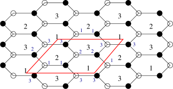
(a) Dimer Diagram

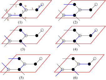
(b) Perfect matchings

Figure 1: Dimer model and perfect matchings for the orbifold $\mathbb{C}^{3}/\mathbb{Z}_{3}$

The Kasteleyn matrix [11] will be

$$K(Z,W)=\pmatrix{a11&a12W&a13Z\cr a21&a22&a23\cr{a31\over Z}&a32&{a33\over W}}$$ (12)

where $aij$ is the label which keeps track of the edge connecting the $i$-th white node to the $j$-th black node and the nodes have been numbered in fig. 1(a). The determinant of $K(W,Z)$ will give six terms corresponding to the six perfect matchings:

$$det~{}K = -a13a22a31+a12a23a31{W\over Z}-a11a23a32-a12a21a33+a13a21a32Z+$$

$$a11a22a33{1\over W}~{}.$$ (13)

The last term, for example, is an algebraic representation of the second perfect matching shown in fig. 1(b). In non-trivial toric Calabi-Yau geometries where the number of perfect matchings is large, the algebraic way of representing perfect matchings makes it easier to determine face symmetries.

The matching matrix (6) is

$${\cal M}=\pmatrix{&p_{1}&p_{2}&p_{3}&p_{4}&p_{5}&p_{6}\cr X_{1}&0&1&0&0&1&0\cr X_{2}&1&1&0&0&0&0\cr X_{3}&0&1&0&0&0&1\cr X_{4}&1&0&0&1&0&0\cr X_{5}&0&0&0&1&1&0\cr X_{6}&0&0&0&1&0&1\cr X_{7}&0&0&1&0&0&1\cr X_{8}&0&0&1&0&1&0\cr X_{9}&1&0&1&0&0&0}$$ (14)

and the charge matrix $Q_{F}$ can be calculated to be

$$Q_{F}=\left(1,-1,-1,-1,1,1\right)$$ (15)

so that the masterspace [13] for this theory is the space $\mathbb{C}^{6}$ modded out by a $U(1)$ with the above charges. Let us now check the two conjectures mentioned in the last section, for this example. First, we discuss the second conjecture regarding the face symmetries. From the closed string point of view, our main observation is that any symmetry associated with the dimer covering should necessarily involve combinations of perfect matchings which force the total closed string R-charge to zero. A symmetry associated with a particular face in the dimer covering is thus equivalent to the closed string R-charges vanishing around that face. This can be seen from fig.1(a). We look for a minimum number of perfect matchings whose combination will enclose the face. Interestingly, the face symmetries are most easily obtained by taking pairwise differences of the internal perfect matchings (corresponding to the twisted sector charge $\left(\frac{1}{3},\frac{1}{3},\frac{1}{3}\right)$). These faces $F_{a}$’s are given by the combinations $F_{1}=p_{5}-p_{6}$, $F_{2}=p_{1}-p_{5}$, and $F_{3}=p_{6}-p_{1}$, where the subscript on $p$ refers to the matching numbers as in fig. (1). Given the labeling of the edges in fig. (1), conjecture 1 of the last section can now be easily shown to yield the quiver charge matrix for the orbifold $\mathbb{C}^{3}/\mathbb{Z}_{3}$

$$d=\pmatrix{&X_{1}&X_{2}&X_{3}&X_{4}&X_{5}&X_{6}&X_{7}&X_{8}&X_{9}\cr F_{1}&1&0&-1&0&1&-1&-1&1&0\cr F_{2}&-1&1&0&1&-1&0&0&-1&1\cr F_{3}&0&-1&1&-1&0&1&1&0&-1\cr}$$ (16)

We now turn to the orbifold $\mathbb{C}^{3}/\mathbb{Z}_{5}$, with the orbifolding action being

$$\left(Z^{1},Z^{2},Z^{3}\right)\to\left(\omega Z^{1},\omega Z^{2},\omega^{3}Z^{3}\right)$$ (17)

where $\omega=e^{\frac{2\pi i}{5}}$. This is the simplest case where there are two internal points in the toric diagram. These correspond to the two marginal twisted sectors in the closed string theory, with twisted sector R-charges $\left(\frac{1}{5},\frac{1}{5},\frac{3}{5}\right)$ and $\left(\frac{2}{5},\frac{2}{5},\frac{1}{5}\right)$ [14]. Inserting these points in the $\mathbb{Z}^{\oplus 3}$ lattice along with the unit vectors, the toric diagram is obtained as shown in fig. (2). Note that the two internal points marked $a$ and $b$ in Fig. 2 are with multiplicity $5$ and $5$. The dimer model for this orbifold is shown in fig. (3).

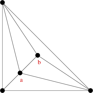
Figure 2: Toric diagram for the supersymmetric orbifold $\mathbb{C}^{3}/\mathbb{Z}_{5}$.

In the appendix, for completeness, we have listed the $10$ internal perfect matchings for the orbifold $\mathbb{C}^{3}/\mathbb{Z}_{5}$ [14] in fig. (15). In this case, there are two types of perfect matchings (corresponding to the two marginal twisted sectors mentioned above). Looking for a minimum number of perfect matching enclosing a face, we confine to pair wise differences. It is not difficult to see that such face symmetries will involve either of the two sets of internal perfect matchings. Also, the fact that the twisted sector $R$-charge vanishes along a face reinforces that there is no mixing between the two sets of internal perfect matchings.

In this example, from fig. (15), it can be seen that the face symmetries can be constructed either by the difference in matchings $p_{1}-p_{7}$, $p_{2}-p_{4}$, $p_{7}-p_{5}$ and $p_{5}-p_{2}$, or, equivalently, from the matchings $p_{10}-p_{3}$, $p_{8}-p_{9}$, $p_{3}-p_{8}$ and $p_{6}-p_{10}$. Both these choices can be seen to give rise to the same quiver charges. The same analysis goes through for orbifold toric diagrams with multiple interior points, and the face symmetries can be written down with perfect matchings corresponding to a single marginal twisted sector. Given that for orbifolds of the form $\mathbb{C}^{3}/\mathbb{Z}_{n}$, twisted sectors appear as internal points in the toric diagram, this means that for generic orbifold theories, the face symmetries are given by combinations of internal points only. We will see in the next section that this is true for non-cyclic orbifolds as well, and we conjecture that this is also true for non-orbifold theories with internal points.

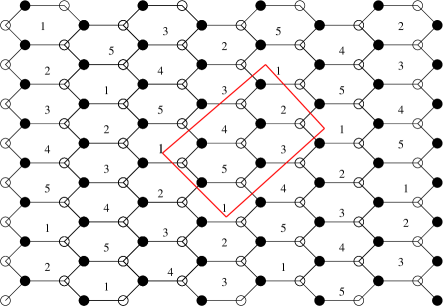
Figure 3: The dimer model for the supersymmetric orbifold $\mathbb{C}^{3}/\mathbb{Z}_{5}$, with the fundamental cell is shown in red.

Before we end this section, let us briefly point out another interesting aspect of dimer model combinatorics as applied to cyclic orbifolds, using the closed string approach.

3.2 Exploring different regions in Kähler moduli space

Let us first consider the orbifold $\mathbb{C}^{3}/\mathbb{Z}_{5}$ as an example (we momentarily generalise the results to generic $\mathbb{Z}_{n}$ orbifold theories). The orbifolding action on the coordinates is

$$\left(Z^{1},Z^{2},Z^{3}\right)\to\left(\omega Z^{1},\omega Z^{2},\omega^{3}Z^{3}\right)$$ (18)

where $\omega=e^{\frac{2\pi i}{5}}$. $\mathbb{C}^{3}/\mathbb{Z}_{5}$ has a closed string $U(1)$ GLSM description in terms of four fields $\phi_{i},i=1,\cdots,4$ with $U(1)$ charges

$$Q=\left(1,1,3,-5\right)$$ (19)

There is a single D-term constraint in the theory,

$$|\phi_{1}|^{2}+|\phi_{2}|^{2}+3|\phi_{3}|^{2}-5|\phi_{4}|^{2}+r=0$$ (20)

where for $r\gg 0$, the field $\phi_{4}$ acquires a large positive value, which breaks the $U(1)$ symmetry into a $\mathbb{Z}_{5}$, and the massless fields $\phi_{i},i=1,2,3$ transform according to the unbroken $\mathbb{Z}_{5}$ symmetry. In the opposite limit $r\ll 0$, the theory is given by a line bundle over a suitable weighted projective space [21]. At other points in Kähler moduli space, there might also be a local orbifold singularity, where the orbifolding action involves the discrete group $\mathbb{Z}_{3}$, or the theory might look like flat space. These can be seen by splitting the toric diagram of fig. (2) from the point denoted as a. This gives rise to three triangles, two of which do not contain an internal point (and hence represent the flat space $\mathbb{C}^{3}$) and the third one has one internal point, marked b in fig. (2) and is identified with the orbifold $\mathbb{C}^{3}/\mathbb{Z}_{3}$. We can equivalently split the toric diagram from point b, and this can be interpreted as the case corresponding to the orbifolding action $\left(Z^{1},Z^{2},Z^{3}\right)\to\left(Z^{1},\omega^{2}Z^{2},\omega^{2}Z^{3}\right)$, where $\omega$ is the fifth root of unity. We will focus on the first case here. It is possible to understand this from a dimer model perspective. Let us see if we can substantiate this. Consider the fundamental region for the dimer covering of the orbifold $\mathbb{C}^{3}/\mathbb{Z}_{5}$ redrawn from fig. (3) in fig. (4)

Figure 4: The fundamental region for the dimer model for the orbifold $\mathbb{C}^{3}/\mathbb{Z}_{5}$, redrawn from fig. (3)

Purely from a combinatorial viewpoint (distinct from Higgsing the theory as in [22]), note that the fundamental region in fig. (4) can be thought of as a gluing of three separate pieces which also qualify as fundamental regions of orbifolds of lower rank - namely, the lower hexagon consisting of the nodes $1$ to $6$, with three external lines, i.e a total of $9$ bifundamentals, the points $7$ and $8$, and the points $9$ and $10$, with both the latter ones having three bifundamental fields each associated to them. However, now the leg from node $6$ has to be identified with node $3$. The latter process can be thought of as the analogue of normalisation of $U(1)$ charges upon reduction of the orbifolding group [20]. This can be generalised as follows. A cyclic orbifold $\mathbb{C}^{3}/\mathbb{Z}_{n}$ will contain, in the fundamental domain of its perfect matching, $2n$ nodes corresponding to the $2n$ terms in the superpotential, and $3n$ bifundamental fields. In order to construct other locally orbifold theories at different points in the Kähler moduli space, we split the original domain into three parts at a given node (for instance node 7 for $\mathbb{Z}_{5}$ as shown in fig. (4)), with each of these parts carrying one of the three edges associated to that node, with the constraint that the three resulting parts have an even number of nodes and an odd number of edges. The latter constraint is required to make the resulting theories $\mathbb{C}^{3}$ orbifolds (or flat space). This generically gives us the theories corresponding to splitting the toric diagram along one of its internal points. This procedure can be seen to go through for higher rank orbifolding groups as well, which might have more than one distinct orbifolding action.

Let us summarise our discussion so far. We have studied the supersymmetric orbifolds of the form $\mathbb{C}^{3}/\mathbb{Z}_{n}$ using a combination of open string and closed string methods. We saw that any symmetry associated to the dimer model implies the vanishing of the total closed string R-charge (a subset of which gives the face symmetries). For toric (cyclic) orbifolds with more than one internal point, these symmetries can be constructed out of any given type of internal point corresponding to a particular R-charge. We will see in the next section that this result is valid for non-cyclic orbifolds as well. Further, we expect that for non-orbifold theories also, the face symmetries can be constructed out of internal points only, whenever these are present. We have also seen that data about the (local) orbifolds of lower rank corresponding to different points in the Kähler moduli space of the original theory are encoded in the dimer covering of the higher rank theory, and can be analysed by splitting (or equivalently gluing) sub diagrams along nodes. These are the main results of this section. We now study some aspects of non cyclic orbifolds of $\mathbb{C}^{3}$.

4 Non cyclic orbifolds of $\mathbb{C}^{3}$

In this section, we will study some simple non-cyclic orbifolds of $\mathbb{C}^{3}$, whose partial resolutions generically give non-orbifold theories. From the point of view of dimer coverings, partial resolutions can be obtained by removing edges from the dimer diagram, which corresponds to a Higgsing process in the D-brane gauge theory [9]. Our aim in this section will be to study these in some details. As is known, arbitrary removal of edges from a dimer model may not correspond to physical D-brane gauge theories. First of all, we note that from the field theory point of view, the Higgsing procedure will not be meaningful if we remove two adjacent edges from a dimer diagram (i.e edges that meet at a single node). Hence, we can eliminate this possibility by giving vevs to edges that do not meet at a node. Even then, the theory is not guaranteed to be consistent, as we will see. An easy way to check consistency of the gauge theory is to derive the superpotential of the resulting theory after Higgsing. A consistent superpotential is one in which the open string modes appear exactly twice, and as we will see in the next few subsections, even after removing non-adjacent edges from a dimer covering, the resulting theory might have an inconsistent superpotential. Unfortunately, there is no general prescription to a priori determine the set of physical gauge theories that might arise due to Higgsing, and one has to proceed on a case to case basis.

In discussing partial resolutions of abelian orbifolds, we will use directly the matching matrix for the “parent” theory (which will give us the various partially resolved “daughter” theories). Indeed the Higgsing procedure can be simply implemented by starting with the full matching matrix ${\cal M}$ (whose rows we label by the fields on the probe D-brane world volume and the columns are the perfect matchings in which these fields occur), and then directly removing those rows which correspond to fields that acquire vevs, and the columns that have non-zero entries corresponding to these rows. This will give us the reduced matching matrix for the partially resolved singularity, from which the gauge theory data can be read off by a prescription similar to the inverse algorithm due to [15]. Namely, following the notation conventions of section (2), given the reduced matching matrix $M_{r}$, we calculate the redundancy matrix $Q_{F(r)}$, whose kernel gives us the reduced $T$ matrix, which we label by $T_{r}$. The dual of the matrix $T_{r}$ is the reduced $K$ matrix (of section 2) inherited by the (partially resolved) daughter singularity. This now can be integrated to give the superpotential of the reduced (non-orbifold) theory. In order to avoid notational complications, we will denote the reduced $K$ matrix of the daughter singularities by the symbol ${\cal K}_{r}$. It will be understood that the reduced matching matrices for these are obtained from ${\cal M}_{r}={\cal K}_{r}^{t}.T_{r}$. In this procedure, one can work directly in terms of the fields in the D-brane gauge theory, and the Higgsing procedure, whenever physical in the sense of the previous paragraph, is guaranteed to give us a resulting physical gauge theory.

The difficulty with the above procedure seems to be that it is incapable of handling adjoint fields, and these have to be added by hand in order to obtain a consistent superpotential [15]. In the field theory, this can be understood by looking at the transformation properties of the massless modes after the Higgsing procedure; in the dimer model description, the equivalent statement is that in the matching matrix, the number of non-zero field entries in any perfect matching is always the same. E.g, for orbifolds, the total number of edges participating in a perfect matching is always $n$, where $n$ is the rank of the orbifolding group. It is easy to see that the same statement goes over for non-orbifold theories as well. This will be useful for us in what follows in order to describe theories that give rise to one or more adjoint fields upon Higgsing.

4.1 The $\mathbb{C}^{3}/\mathbb{Z}_{2}\times\mathbb{Z}_{2}$ singularity

Let us begin this subsection with an analysis for the orbifold $\mathbb{C}^{3}/\mathbb{Z}_{2}\times\mathbb{Z}_{2}$, with the orbifolding action being

$$g_{1}:\left(Z_{1},Z_{2},Z_{3}\right)\to\left(-Z_{1},-Z_{2},Z_{3}\right)$$

$$g_{1}:\left(Z_{1},Z_{2},Z_{3}\right)\to\left(-Z_{1},Z_{2},-Z_{3}\right)$$ (21)

where the $Z_{i},i=1,2,3$ denote the coordinates of $\mathbb{C}^{3}$. In the closed string description of this orbifold, we consider the $\mathbb{Z}^{\oplus 3}$ lattice generated by the basis vectors ${\vec{e}_{1}}=(1,0,0)$, ${\vec{e}_{2}}=(0,1,0)$ and ${\vec{e}_{3}}=(0,0,1)$, and augment them with the fractional points that correspond to the R-charges (of the closed string twist operator) of the three marginal sectors of the theory. These are given by the vectors ${\vec{e}_{4}}=(\frac{1}{2},0,\frac{1}{2})$, ${\vec{e}_{5}}=(\frac{1}{2},\frac{1}{2},0)$, ${\vec{e}_{6}}=(0,\frac{1}{2},\frac{1}{2})$ and correspond to the action by $g_{1}$, $g_{2}$ and $g_{1}.g_{2}$. The toric diagram for the orbifold is shown in fig. (5). In the same figure, we have also shown the position of the lattice vectors ${\vec{e}_{1}},\cdots,{\vec{e}_{6}}$, along with their multiplicities in the brane probe picture [15], and a partial resolution of this to the non-orbifold SPP singularity.

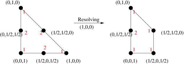
Figure 5: Toric diagram for the partial resolution of the singularity $\mathbb{C}^{3}/\mathbb{Z}_{2}\times\mathbb{Z}_{2}$ to the SPP singularity. We have also shown the closed string R-charges of the parent orbifold theory in both the diagrams.

In fig. (6), we show the dimer model for this singularity, and its perfect matchings. The perfect matchings are classified according to their closed string twisted sector R charges, which can be read off by assigning weights to the edges of the original hexagonal lattice [14]. These have also been shown in fig. (6), where we have assigned weights to the edges according to their orientation, with the condition that three different types of edges meet at each vertex. From fig. (6), we can read off the matching matrix for the $\mathbb{C}^{3}/\mathbb{Z}_{2}\times\mathbb{Z}_{2}$ singularity, and it is given by

$${\cal M}=\pmatrix{~{}&p_{1}&p_{2}&p_{3}&p_{4}&p_{5}&p_{6}&p_{7}&p_{8}&p_{9}\cr x1&1&0&0&1&0&1&0&0&0\cr x2&1&0&0&0&1&0&1&0&0\cr x3&1&0&0&1&0&0&1&0&0\cr x4&1&0&0&0&1&1&0&0&0\cr y1&0&1&0&0&0&1&0&0&1\cr y2&0&1&0&0&0&0&1&1&0\cr y3&0&1&0&0&0&0&1&0&1\cr y4&0&1&0&0&0&1&0&1&0\cr z1&0&0&1&1&0&0&0&0&1\cr z2&0&0&1&0&1&0&0&1&0\cr z3&0&0&1&1&0&0&0&1&0\cr z4&0&0&1&0&1&0&0&0&1\cr}$$ (22)

where the rows denote the $12$ surviving bifundamental fields in the D-brane gauge theory after the orbifold projection, and we have explicitly labeled these by the edge numbers appearing in fig. (6), and the columns correspond to the perfect matching number which has been given in that figure.

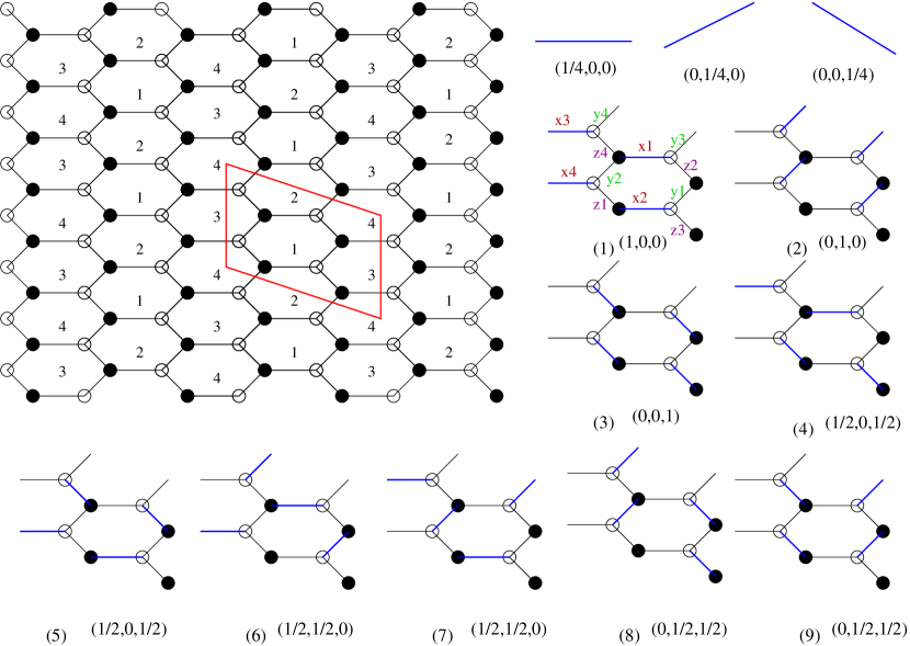
Figure 6: The fundamental domain and the perfect matchings for the singularity $\mathbb{C}^{3}/\mathbb{Z}_{2}\times\mathbb{Z}_{2}$. We have also shown the labeling for the edges, which correspond to bifundamental fields in the gauge theory.

From the closed string perspective, since the toric diagram in this case does not contain any internal point, each face symmetry (three such symmetries are independent as can be seen from the dimer diagram) must necessarily involve one corner point of the diagram, and three other points. It is easy to write these down, as combinations of the points in the toric diagram that sum up to zero closed string R-charge, in the spirit of the last section, and one possible choice for these combinations is

$${\vec{e}_{1}}-{\vec{e}_{4}}-{\vec{e}_{5}}+{\vec{e}_{6}} = 0$$

$${\vec{e}_{2}}+{\vec{e}_{4}}-{\vec{e}_{5}}-{\vec{e}_{6}} = 0$$

$${\vec{e}_{3}}-{\vec{e}_{4}}+{\vec{e}_{5}}-{\vec{e}_{6}} = 0$$ (23)

Now, from the matching matrix ${\cal M}$ of eq. (22), we can obtain its redundancy matrix, which is, in the case, a $3\times 9$ matrix. The set of face symmetries can be obtained directly from ${\cal M}$ by noting from fig. (6) that these symmetries involve the edges

$$F1:\left(x1,x2,y1,y2,z1,z2\right);~{}~{}~{}F2:\left(x1,x2,y3,y4,z3,z4\right);~{}~{}~{}F3:\left(x3,x4,y1,y2,z3,z4\right)$$ (24)

Combinations of the perfect matchings that give this set of edges can be constructed from the columns of the matching matrix by forming linear combinations whose only nonzero (unit) entries are at the positions of the above edges. In this case, it can be checked that one possible choice of these combinations for the faces $F1,F2,F3$ are respectively,

$$p3-p5+p6-p8;~{}~{}~{}p2+p5-p6-p8;~{}~{}~{}p1-p5-p6+p8$$ (25)

These are of course equivalent to the combinations in eq. (23). The signs are chosen so that each face is traversed in clockwise sense. This information can then be used to construct the quiver diagram for the singularity $\mathbb{C}^{3}/\mathbb{Z}_{2}\times\mathbb{Z}_{2}$ in a standard manner, following eq. (9). Let us now study the partial resolutions of the $\mathbb{C}^{3}/\mathbb{Z}_{2}\times\mathbb{Z}_{2}$ singularity. This is interesting, because in this case, partial resolutions give rise to massless adjoint fields.

We begin with the matching matrix ${\cal M}$ of $\mathbb{C}^{3}/\mathbb{Z}_{2}\times\mathbb{Z}_{2}$, given in eq. (22). In order to remove one corner of the toric diagram of fig. (5), we proceed by removing the row $x1$ of ${\cal M}$. This gives the partial resolution of the parent singularity to the suspended pinch point (SPP), as shown in fig. (5). Let us now understand the combinatorial description of this process. Removing the edge $x1$ gives us a reduced matching matrix, which can be constructed by directly deleting the first row and the first, fourth and sixth columns of ${\cal M}$. The reduced charge matrix is now given by the kernel of the reduced matching matrix,

$$Q_{F(r)}=\left(-1,-1,0,0,1,1\right)$$ (26)

The dual of the kernel of $Q_{r}$ (which is the $5\times 6$ matrix $T_{r}$) is given by the set of vectors

$${\cal K}_{r}=\pmatrix{0&0&0&0&1&1\cr 0&0&1&1&0&0\cr 0&1&0&0&0&0\cr 1&0&0&0&0&0\cr 0&0&0&1&0&1\cr}$$ (27)

Hence, removing the edge $x1$ has resulted in the removal of $5$ more edges, i.e a total of $6$ edges out of the initial $12$ have been removed (so that we have a resulting graph with six remaining edges). In a Higgsing procedure, one would expect that a total of five edges get removed on removing one of the edges of the graph for the parent singularity. The matrix of eq. (27) therefore signals the appearance of an adjoint field. Note that the superpotential calculated from ${\cal K}_{r}$ is inconsistent. Further, if we went ahead with this matrix ${\cal K}_{r}$ and calculated the resulting matching matrix, the result would be

$${\cal M}_{r}=\pmatrix{0&0&1&0&0&0\cr 0&0&0&1&0&0\cr 1&0&0&0&1&0\cr 0&1&0&0&1&0\cr 1&0&0&0&0&1\cr 0&1&0&0&0&1\cr}$$ (28)

with now the rows denoting the new edges and the columns labeling the perfect matchings in the new graph corresponding to the SPP singularity. As a perfect matching matrix, eq. (28) is clearly inconsistent. This is because the same number of bifundamental fields do not appear in each perfect matching. The observation here is that we can remedy the situation by inserting an extra column in eq. (27), (corresponding to the adjoint field), so that the rows in the matrix ${\cal K}_{r}$ are forced to add up to the same integer ($2$ in this case). On applying this modification, we arrive at the matrix

$${\cal K}_{r}^{\prime}=\pmatrix{0&0&0&0&1&1&0\cr 0&0&1&1&0&0&0\cr 0&1&0&0&0&0&1\cr 1&0&0&0&0&0&1\cr 0&0&0&1&0&1&0\cr}$$ (29)

where now the seven columns refer to the seven fields in the theory with the last column being the added adjoint. This can be integrated to give the superpotential

$$W_{spp}=X_{1}X_{2}X_{3}X_{6}-X_{1}X_{2}X_{4}X_{5}+X_{3}X_{6}X_{7}-X_{4}X_{5}X_{7}$$ (30)

This is now seen to match with the result of [19], with the $X_{i},i=1,\cdots 7$ being the bifundamentals in the D-brane gauge theory of the SPP singularity, and in terms of these fields, the matching matrix for the SPP singularity is seen to be

$${\cal M}_{spp}=\pmatrix{~{}&{\tilde{p}}_{1}&{\tilde{p}}_{2}&{\tilde{p}}_{3}&{\tilde{p}}_{4}&{\tilde{p}}_{5}&{\tilde{p}}_{6}\cr X_{1}&0&0&1&0&0&0\cr X_{2}&0&0&0&1&0&0\cr X_{3}&1&0&0&0&1&0\cr X_{4}&0&1&0&0&1&0\cr X_{5}&1&0&0&0&0&1\cr X_{6}&0&1&0&0&0&1\cr X_{7}&0&0&1&1&0&0\cr}$$ (31)

where the rows $Xi,i=1,\cdots,7$ label the seven bifundamentals and the columns ${\tilde{p}}_{i},i=1,\cdots,6$ denote the six perfect matchings of the partially resolved theory. From the superpotential above, we may construct the dimer diagram for the SPP singularity. This is well known, and shown in fig. (7).

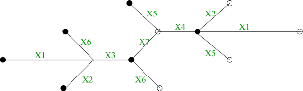
Figure 7: Dimer model for the SPP singularity.

From the new matching matrix of eq. (31), we can construct the face symmetries. From fig. (7), we see that there are three faces, so that only two of them give independent constraints. The set of edges that participate in these face symmetries are given by $\left(X_{1},X_{2},X_{3},X_{6}\right)$ and $\left(X_{1},X_{2},X_{4},X_{5}\right)$. From eq. (31), when the signs are appropriately taken care of (so that the faces are traversed in the same sense), these set of edges correspond to the combinations

$$-{\tilde{p}}_{2}+{\tilde{p}}_{3}-{\tilde{p}}_{4}+{\tilde{p}}_{5}~{}~{}~{}{\rm and}~{}~{}~{}{\tilde{p}}_{1}-{\tilde{p}}_{3}+{\tilde{p}}_{4}-{\tilde{p}}_{5}$$ (32)

where the ${\tilde{p}}_{i},i=1,\cdots,6$ label the columns of ${\cal M}_{spp}$. Forming the matrix

$$A=Q_{D(spp)}=\pmatrix{0&-1&1&-1&1&0\cr 1&0&-1&1&-1&0\cr}$$ (33)

we obtain the matrix $Q_{D(spp)}.{\cal M}^{T}_{spp}=d$, from which, removing the redundant $U(1)$ gives

$${\Delta}_{spp}=\pmatrix{1&-1&1&0&0&-1&0\cr-1&1&0&-1&1&0&0\cr}$$ (34)

which correctly describes the quiver for the SPP. Equivalently, one could have directly calculated the quiver charges from eq. (9).

Let us now move to our next example, where we remove a further edge from the $\mathbb{C}^{3}/\mathbb{Z}_{2}\times\mathbb{Z}_{2}$ singularity. This can be achieved conveniently by removing, say, the first row (and thus the third column) from the matching matrix for the SPP, ${\cal M}_{spp}$, given in eq. (31). It can be checked that this is equivalent to directly removing the bifundamentals denoted by $x1$ and $x4$ from the matching matrix of $\mathbb{C}^{3}/\mathbb{Z}_{2}\times\mathbb{Z}_{2}$ given in eq. (22). This imples that (from the toric diagram), we are left with the singularity $\mathbb{C}^{2}/\mathbb{Z}_{2}\times\mathbb{C}$. The dual of the kernel of the redundancy matrix in this case is given by

$${\cal K}_{r}^{\prime\prime}=\pmatrix{0&0&0&1&1\cr 0&1&1&0&0\cr 1&0&0&0&0\cr 0&0&1&0&1\cr}$$ (35)

The perfect matching matrix here suffers from the same inconsistency as before, and hence we introduce one more adjoint field to write down the modified matrix

$${\cal K}_{\mathbb{C}^{2}/\mathbb{Z}_{2}\times\mathbb{C}}=\pmatrix{0&0&0&1&1&0\cr 0&1&1&0&0&0\cr 1&0&0&0&0&1\cr 0&0&1&0&1&0\cr}$$ (36)

which gives us the superpotential

$$W_{\mathbb{C}^{2}/\mathbb{Z}_{2}\times\mathbb{C}}=X_{1}X_{2}X_{5}-X_{1}X_{3}X_{4}+X_{2}X_{5}X_{6}-X_{3}X_{4}X_{6}$$ (37)

A computation analogous to that for the SPP (or using eq. (9)) now yields the quiver charge matrix

$$\Delta_{\mathbb{C}^{2}/\mathbb{Z}_{2}\times\mathbb{C}}=\left(0,1,-1,1,-1,0\right)$$ (38)

which tells us that the fields $X_{1}$ and $X_{6}$ are adjoints.

Before we conclude this subsection, we briefly comment on the resolution of the $\mathbb{C}^{3}/\mathbb{Z}_{2}\times\mathbb{Z}_{2}$ singularity to the conifold. As is known, this theory does not have F-terms and the entire information of the gauge theory is contained in the D-term equations. We can see this from the matching matrix of eq. (22). In order to reach the conifold singularity from the original matching matrix, we can remove the bifundamentals denoted by $x1$ and $y1$. Eq. (22) then tells us that along with these fields, five of the nine perfect matchings have to be removed, and we are left with a theory that has four perfect matchings. However, the redundancy matrix corresponding to the $7\times 4$ matrix that remain after this removal is the null matrix $0_{1\times 4}$. Hence, we can take the $T_{r}$ matrix in this case as the matrix ${\rm Id}_{4\times 4}$, whose dual matrix ${\cal K}_{r}$ is again the $4\times 4$ identity matrix. The matching matrix for the conifold is thus ${\rm Id}_{4\times 4}$. The dimer covering and the perfect matchings can now be constructed in a standard way, and eq. (9) can be implemented in a standard manner to give rise to the charge matrix

$$\Delta_{conifold}=\pmatrix{1&-1&-1&1\cr}$$ (39)

As a final remark, note that at each stage, the toric diagrams of the resolutions can be obtained by constructing the perfect matchings, whose information is contained in the matching matrix, and constructing their height functions. Equivalently, this can be done by directly removing points from that of the parent singularity corresponding to the bifundamentals that are removed.

We now discuss the singularity $\mathbb{C}^{2}/\mathbb{Z}_{2}\times\mathbb{Z}_{3}$. This is the next nontrivial example where adjoint fields appear on partial resolutions of the singularity.

4.2 The Singularity $\mathbb{C}^{3}/\mathbb{Z}_{2}\times\mathbb{Z}_{3}$

In this subsection, we study the orbifold $\mathbb{C}^{2}/\mathbb{Z}_{2}\times\mathbb{Z}_{3}$, where the orbifolding group implies an asymmetric action on the coordinates. We will see how the computational tools introduced in the last subsection can be effectively used in this context as well. The closed string description of this orbifold parallels the one discussed in the last subsection. Specifically, we choose the action of the orbifolding group on the coordinates as

$$g_{1}=\left(Z_{1},Z_{2},Z_{3}\right)\to\left(-Z_{1},Z_{2},-Z_{3}\right)$$

$$g_{2}=\left(Z_{1},Z_{2},Z_{3}\right)\to\left(\omega Z_{1},\omega^{2}Z_{2},Z_{3}\right)$$ (40)

where $\omega=e^{\frac{2\pi i}{3}}$ and the $Z_{i},i=1,2,3$ are the coordinates of $\mathbb{C}^{3}$. Taking into account the various marginal twisted sectors (in addition to the generators of an $SL(3,Z)$ lattice), we obtain the toric diagram shown in fig. (8) (after projection to a convenient plane, so that the vectors are coplanar). In fig. (8), we have also marked the closed string R-charges.

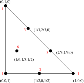
Figure 8: Toric diagram for the singularity $\mathbb{C}^{3}/\mathbb{Z}_{2}\times\mathbb{Z}_{3}$. The closed string R-charges are shown, along with the multiplicities of the fields in the open string picture.

The fundamental region for the dimer model for this singularity is shown in fig. (9).

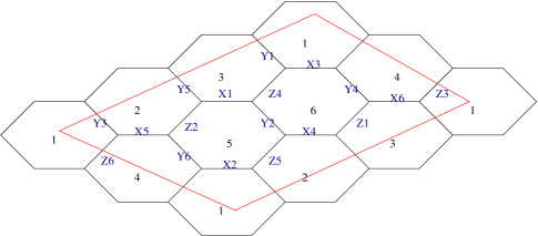
Figure 9: Fundamental region for the dimer model of the singularity $\mathbb{C}^{3}/\mathbb{Z}_{2}\times\mathbb{Z}_{3}$. We have labeled the edges in accordance with the previous subsection.

In the appendix, we have shown diagrammatically the $17$ possible perfect matchings for the dimer model of this singularity. These can be obtained by using the Kasteleyn matrix, as in the last section. Also, in the appendix, we have provided the matching matrix for this singularity in eq. (61), where the $18$ surviving bifundamental fields of this theory have been collectively labelled as $X_{i},i=1,\cdots,18$. From this matrix, we can see that due to the asymmetric action of the orbifold, removing different nodes may result in the removal of different number of perfect matchings during Higgsing. Again, the face symmetries correspond to the total closed string R-charge vanishing around each face. These are also seen to be combinations only of the perfect matchings corresponding to the internal point in the toric diagram of fig. (8). Let us now consider some blowups of this singularity, via the Higgsing procedure from the dimer model perspective. These have been previously considered in [19]. First, we give a vev to one of the fields, in eq. (61), say $X_{1}$. The charge matrix for the reduced singularity is found to be

$$Q^{1}_{F(r)}=\pmatrix{-1&1&0&0&0&-1&-1&1&0&0&1\cr 0&-1&0&0&-1&0&1&0&0&1&0\cr 1&-1&-1&0&-1&1&1&-1&1&0&0\cr 1&-1&-1&1&0&0&0&0&0&0&0\cr}$$ (41)

This gives rise to the reduced $K$ matrix, now with $13$ fields,

$${\cal K}^{1}_{r}=\pmatrix{0&0&0&0&0&0&0&0&0&1&1&1&1\cr 0&0&0&0&0&0&1&1&1&0&0&0&1\cr 0&0&0&1&1&1&0&0&1&0&0&0&0\cr 0&1&1&0&1&1&0&0&0&0&0&0&0\cr 1&0&1&0&0&1&0&0&0&0&0&1&0\cr 0&1&0&0&0&0&0&1&0&0&1&0&1\cr 0&0&0&0&0&1&0&0&1&0&0&1&1\cr}$$ (42)

which can be integrated to give the superpotential

$$W= Y_{1}Y_{5}Y_{13}-Y_{3}Y_{4}Y_{13}+Y_{3}Y_{9}Y_{11}-Y_{5}Y_{8}Y_{12}-Y_{6}Y_{7}Y_{11}+Y_{6}Y_{8}Y_{10}$$ (43)

$$- Y_{1}Y_{2}Y_{9}Y_{10}+Y_{2}Y_{4}Y_{7}Y_{12}$$

where we have labeled the new fields as $Y_{i},i=1,\cdots 13$ to avoid confusion. The reduced matching matrix now involves $13$ bifundamentals and $11$ perfect matchings, and is given by

$${\cal M}^{1}_{r}=\pmatrix{~{}&{\tilde{p}}_{1}&{\tilde{p}}_{2}&{\tilde{p}}_{3}&{\tilde{p}}_{4}&{\tilde{p}}_{5}&{\tilde{p}}_{6}&{\tilde{p}}_{7}&{\tilde{p}}_{8}&{\tilde{p}}_{9}&{\tilde{p}}_{10}&{\tilde{p}}_{11}\cr Y_{1}&0&1&0&1&0&0&1&0&0&0&0\cr Y_{2}&0&0&0&0&0&1&0&1&0&0&0\cr Y_{3}&1&1&0&0&0&0&1&1&0&0&0\cr Y_{4}&0&0&1&1&0&0&0&0&1&0&0\cr Y_{5}&1&0&1&0&0&0&0&1&1&0&0\cr Y_{6}&0&0&0&0&1&0&1&1&1&0&0\cr Y_{7}&1&1&0&0&0&0&0&0&0&1&0\cr Y_{8}&0&1&0&1&0&1&0&0&0&1&0\cr Y_{9}&0&0&0&0&1&0&0&0&1&1&0\cr Y_{10}&1&0&1&0&0&0&0&0&0&0&1\cr Y_{11}&0&0&1&1&0&1&0&0&0&0&1\cr Y_{12}&0&0&0&0&1&0&1&0&0&0&1\cr Y_{13}&0&0&0&0&1&1&0&0&0&1&1\cr}$$ (44)

Where now the ${\tilde{p}}_{i},i=1\cdots 11$ are the new perfect matchings that descend from the parent theory. The dimer model for this partial resolution of $\mathbb{C}^{3}/\mathbb{Z}_{2}\times\mathbb{Z}_{3}$ is shown in fig. 10 a.

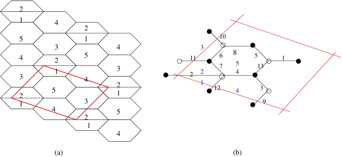
Figure 10: Dimer covering for the gauge theory for the orbifold $\mathbb{C}^{3}/\mathbb{Z}_{2}\times\mathbb{Z}_{3}$ with the edge $X_{1}$ removed. In (a), we have shown the fundamental domain of this covering. (b) shows a labeling of the bifundamental fields corresponding to the superpotential in eq. (43) (in black). The blue colored integers in (b) refer to the original labeling of the faces in (a).

From fig. (10 a), we can directly draw the toric diagram, or, in the spirit of the previous subsection, note that the five distinct faces of the dimer diagram in the figure are generated by the bifundamentals

$$F1 = \left(Y_{2},Y_{8},Y_{10},Y_{12}\right),~{}~{}F2=\left(Y_{2},Y_{7},Y_{9},Y_{11}\right),~{}~{}F3=\left(Y_{1},Y_{3},Y_{6},Y_{10},Y_{11},Y_{13}\right),$$

$$F4 = \left(Y_{1},Y_{3},Y_{4},Y_{5},Y_{9},Y_{12}\right),~{}~{}F5=\left(Y_{4},Y_{5},Y_{6},Y_{7},Y_{8},Y_{13}\right)$$ (45)

This implies that the face symmetries are generated by the matrix

$$Q_{D}^{1}=\pmatrix{~{}&1&0&0&0&0&-1\cr~{}&-1&0&0&0&1&0\cr 0_{5\times 5}&0&-1&0&0&0&1\cr~{}&0&1&0&-1&0&0\cr~{}&0&0&0&1&-1&0\cr}$$ (46)

from which we read off the quiver matrix

$$d=\pmatrix{1&0&1&-1&-1&0&0&0&-1&0&0&1&0\cr-1&0&-1&0&0&-1&0&0&0&1&1&0&1\cr 0&0&0&1&1&1&-1&-1&0&0&0&0&-1\cr 0&1&0&0&0&0&0&1&0&-1&0&-1&0\cr 0&-1&0&0&0&0&1&0&1&0&-1&0&0\cr}$$ (47)

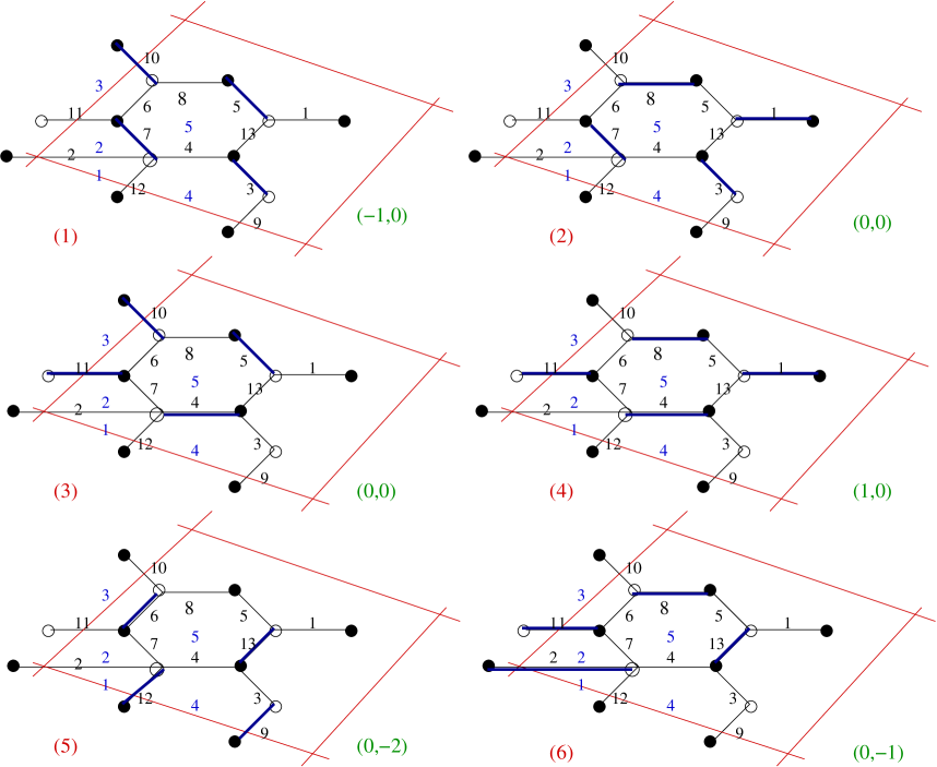
Figure 20: Perfect matchings for the orbifold $\mathbb{C}^{3}/\mathbb{Z}_{2}\times\mathbb{Z}_{3}$ with the field $X_{1}$ of eq. (61) removed. The integers (in red) on the left of each perfect matching correspond to the matching number in the matrix of eq. (44). The height functions are indicated by the green integers on the right.

Now we need to check that the face symmetries are indeed obtainable from purely internal matchings of the toric diagram for this dimer model. This is not difficult to see. In fig. (10 b), we have shown (one choice for) the labeling of the fields that arise in the superpotential of eq. (43). In fig. (20) and (21) in the appendix, we have shown explicitly the eleven perfect matchings corresponding to the matching matrix in eq. (44). From the labeling of the matchings in terms of the height functions, we see that ${\tilde{p}}_{6}$, ${\tilde{p}}_{7}$, ${\tilde{p}}_{9}$, ${\tilde{p}}_{10}$ and ${\tilde{p}}_{11}$ are the five internal matchings, as expected from eq. (46). The toric diagram for this partial resolution is shown in fig. (11).

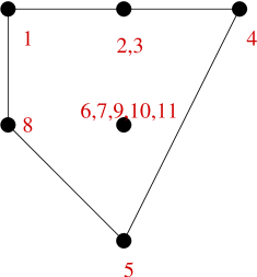
Figure 11: Toric diagram for the orbifold $\mathbb{C}^{3}/\mathbb{Z}_{2}\times\mathbb{Z}_{3}$ with the edge $X_{1}$ removed. The integers in red label the perfect matchings that appear in eq. (44). The positions of these correspond to the height functions as shown in fig. (21) in the appendix.

Consider now a further blowup of this orbifold, wherein we give a vev to the field $Y_{1}$ in eq. (44). The reduced charge matrix is given by

$$Q^{2}_{F(r)}=\pmatrix{0&-1&-1&0&0&1&0&1\cr-1&1&0&-1&1&-1&1&0\cr}$$ (48)

from which we can directly see that this is the cone of the first del Pezzo surface $dP_{1}$ [13], equivalently, this conclusion can be reached by calculating the superpotential which, in this case, can be determined as

$$W=Y_{1}Y_{7}Y_{10}-Y_{2}Y_{7}Y_{8}+Y_{4}Y_{6}Y_{8}-Y_{4}Y_{5}Y_{10}+Y_{2}Y_{3}Y_{5}Y_{9}-Y_{1}Y_{3}Y_{6}Y_{9}$$ (49)

with the $Y_{i},i=1,\cdots 10$ now denoting the bifundamental fields of the new theory. Now, consider giving a vev to the field $Y_{2}$ in eq. (44). In this case, we can calculate the reduced charge matrix to be

$$Q^{3}_{F(r)}=\pmatrix{0&0&-1&0&-1&0&1&0&1\cr 0&-1&0&0&-1&1&0&1&0\cr 1&-1&-1&1&0&0&0&0&0\cr}$$ (50)

This singularity has a toric diagram which can be obtained from that in fig. (11) with the points labeled $6$ and $8$ removed, i.e it is a triangle with one internal point (with multiplicity $4$) and one point on the boundary (with multiplicity $2$). It is known that such toric diagrams with points on the boundary typically arise in orbifolds which might have a non-isolated singularity [23]. Further, in this case, from the charge matrix of eq. (50), the partially resolved theory is seen to contain $12$ bifundamental fields. By explicit computation using the forward algorithm, we have checked that this is in fact the $\mathbb{C}^{3}/\mathbb{Z}_{4}$ singularity. The superpotential obtained from the ${\cal K}_{r}$ matrix computed from eq. (50) also confirms this.

Before we end this subsection, let us consider one more example. Consider removing the edge $Z_{4}$ from the matching matrix of $\mathbb{C}^{3}/\mathbb{Z}_{2}\times\mathbb{Z}_{3}$. It can be checked that this results in an inconsistent superpotential for the resulting theory. Now, we consider removing the bifundamentals $Z_{4}$ and $Z_{6}$ simultaneously. This yields the reduced ${\cal K}_{r}$ matrix, in which we need to add two adjoint fields (to make the resulting matching matrix consistent), and after this, the matrix reads

$${\cal K}^{4}_{r}=\pmatrix{0&0&0&0&0&0&0&1&1&1\cr 0&0&0&0&0&0&1&0&1&1\cr 0&0&0&1&1&1&0&0&0&0\cr 0&1&1&0&0&1&0&0&0&0\cr 1&0&1&0&1&0&0&0&0&0\cr 0&1&0&1&0&1&0&0&0&0\cr}$$ (51)

where the last two columns denote the (adjoint) fields that we have added. For this case, we obtain the superpotential

$$W=Y_{1}Y_{6}Y_{9}-Y_{2}Y_{5}Y_{9}+Y_{3}Y_{4}Y_{10}-Y_{1}Y_{6}Y_{10}+Y_{2}Y_{5}Y_{7}Y_{8}-X_{3}Y_{4}Y_{7}Y_{8}$$ (52)

where $Y_{i},i=1,\cdots 10$ denote the bifundamental fields of the resulting theory. This is seen to match with the corresponding result of [19] after an obvious identification of fields. The quiver charges and the dimer model of this theory can be obtained by standard means outlined before, and we do not present them here. Rather, let us point out a puzzle that we are unable to resolve at this stage. Suppose we give a vev to the fields $Z_{1}$ and $Z_{2}$ instead. It can be checked that this gives rise to exactly the same ${\cal K}_{r}$ matrix as in eq. (51), and hence to the same superpotential with two adjoints. But now the toric diagram of the resulting theory has a multiplicity at an external point, and hence is inconsistent. In fact, from an algebraic analysis, this singularity can be shown to have an equation that is analogous to the singularity $\mathbb{C}^{2}/\mathbb{Z}_{3}\times\mathbb{C}$, which, in the $N=1$ description, should have a matter content of $9$ fields, including $3$ adjoints, which is clearly not the case at hand. The forward algorithm is less useful here, due to the presence of adjoint fields, and apriori we do not know how to rule out this case. We believe that this might be a generic feature of orbifolds of the form $\mathbb{C}^{3}/\mathbb{Z}_{m}\times\mathbb{Z}_{n}$ with $m\neq n$, where removing different bifundamentals may remove different numbers of perfect matchings, and it needs to be investigated further.

4.3 The Orbifold $\mathbb{C}^{3}/\mathbb{Z}_{3}\times\mathbb{Z}_{3}$

We now present our results on the orbifold $\mathbb{C}^{3}/\mathbb{Z}_{3}\times\mathbb{Z}_{3}$. We will be brief here due to space constraints, and also becos our methods of the previous subsection carry over straightforwardly in this case (we do not have any complications due to adjoint fields here). The orbifolding action is

$$g_{1}=\left(Z_{1},Z_{2},Z_{3}\right)\to\left(\omega Z_{1},\omega^{2}Z_{2},Z_{3}\right)$$

$$g_{2}=\left(Z_{1},Z_{2},Z_{3}\right)\to\left(\omega Z_{1},Z_{2},\omega^{2}Z_{3}\right)$$ (53)

where $\omega=e^{\frac{2\pi i}{3}}$ and as usual, $Z_{i},i=1,2,3$ denote the coordinates of $\mathbb{C}^{3}$. The orbifold projection can be carried out in a standard way, and shows that in this case, there are $27$ fields surviving the orbifolding action, and that there are $42$ perfect matchings. Due to space constraints, we have presented only a subset of these matchings in the appendix. In the appendix, we have also presented the matching matrix for this orbifold. From this, one can construct the matching matrix for the completely singular variety, or its partial resolutions. We have again checked that the face symmetries are generated by the perfect matchings that correspond to only internal point in the toric diagram for this singularity, shown in fig. (12). In the closed string description, we consider the $\mathbb{Z}^{\oplus 3}$ lattice, generated by the vectors ${\vec{e}_{1}}=\left(1,0,0\right)$, ${\vec{e}_{2}}=\left(0,1,0\right)$, ${\vec{e}_{3}}=\left(0,0,1\right)$, and include the following seven fractional points ${\vec{e}_{4}},\cdots,{\vec{e}_{10}}$ which correspond to the seven marginal sectors in the theory :

$$\left(\frac{1}{3},\frac{2}{3},0\right),~{}\left(\frac{2}{3},\frac{1}{3},0\right),~{}\left(\frac{1}{3},0,\frac{2}{3}\right),~{}\left(\frac{2}{3},0,\frac{1}{3}\right),$$ (54)

$$\left(0,\frac{1}{3},\frac{2}{3}\right),~{}\left(0,\frac{2}{3},\frac{1}{3}\right),~{}\left(\frac{1}{3},\frac{1}{3},\frac{1}{3}\right)$$

In fig. (12), we have also shown the perfect matchings corresponding to each closed string twisted sector.

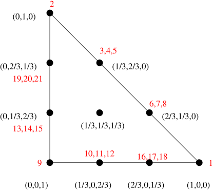
Figure 12: Toric diagram for the resolution of the singularity $\mathbb{C}^{3}/\mathbb{Z}_{3}\times\mathbb{Z}_{3}$. We have shown the closed string R-charges of the of the twisted sectors, as well as the perfect matchings which correspond to them, following our diagrams for this singularity presented in the appendix.

We now discuss some resolutions of this singularity. From the matching matrix for this orbifold presented in the appendix, it can be seen that removal any one edge from the graph removes seven internal and seven external points from the toric diagram. Removing, for example, the bifundamental field $X_{1}$ can be seen to give rise to a theory that has a $18\times 24$ charge matrix, from which the (reduced) $T$ matrix can be calculated, and the dual to this matrix is the reduced ${\cal K}_{r}$ matrix, given by

$${\cal K}_{r}=\pmatrix{0&0&0&0&0&0&0&0&0&0&0&0&0&0&0&1&1&1&1&1&1&1\cr 0&0&0&0&0&0&0&0&0&0&0&1&1&1&1&0&0&0&0&1&1&1\cr 0&0&0&0&0&0&0&0&0&0&1&0&0&1&1&0&0&0&1&1&1&1\cr 0&0&0&0&0&0&0&1&1&1&0&1&1&0&1&0&0&0&0&0&0&1\cr 0&0&0&0&0&1&1&0&0&0&0&1&1&1&0&0&0&0&0&1&1&0\cr 0&0&0&1&1&0&1&0&1&1&0&0&1&0&0&0&0&1&0&0&0&0\cr 0&1&1&0&1&0&0&0&0&0&0&0&0&0&0&1&1&1&0&0&1&0\cr 1&0&1&0&0&1&0&1&0&1&0&1&0&0&0&0&1&0&0&0&0&0\cr 0&0&0&1&0&0&1&0&1&0&0&0&0&0&0&1&0&1&1&1&0&0\cr 1&0&0&1&0&0&1&0&0&0&0&0&0&1&0&0&0&1&1&1&0&0\cr}$$ (55)

and is seen to give the superpotential

$$W = X_{1}X_{9}X_{21}-X_{2}X_{10}X_{20}-X_{3}X_{7}X_{22}+X_{3}X_{13}X_{19}-X_{4}X_{8}X_{21}+X_{5}X_{8}X_{20}-X_{5}X_{12}X_{19}$$ (56)

$$- X_{6}X_{15}X_{18}+X_{7}X_{15}X_{17}-X_{9}X_{14}X_{17}+X_{10}X_{14}X_{16}+X_{11}X_{12}X_{18}$$

$$- X_{1}X_{11}X_{13}X_{16}+X_{2}X_{4}X_{6}X_{22}$$

This gives the dimer covering, which is shown in fig. (13).

Figure 13: Dimer model of the orbifold $\mathbb{C}^{3}/\mathbb{Z}_{3}\times\mathbb{Z}_{3}$ with one bifundamental field removed.

Removal of the edge $X_{1}$ removes one corner of the toric diagram, as above, and in order to remove a further corner, from the matching matrix for the orbifold provided in the appendix, it can be seen that there are fourteen choices for the same. We will just provide the result here. We find that $12$ out of these $14$ choices give rise to consistent superpotentials. These correspond to two of the phases of the $PdP_{4}$ theory (which is the third del Pezzo surface blown up at a generic point) [25]. Specifically, for $8$ cases, we get a toric diagram with $9$ internal points and for $4$ cases, we get a toric diagram with $12$ internal points, the number of external points being $7$ for both. The remaining $2$ choices are seen to give inconsistent superpotentials, although one cannot apriori rule out these cases simply from their toric diagrams. The third phases of $PdP_{4}$ cannot be obtained from this procedure, as pointed out in [25]. Now, one can remove a further corner from the resulting toric diagram, and this straightforwardly gives rise to the four phases of the $dP_{3}$ theory. At each stage, starting from the matching matrix for the $\mathbb{C}^{3}/\mathbb{Z}_{3}\times\mathbb{Z}_{3}$ orbifold, the charges for the masterspaces of these theories and their superpotentials can be read off.

Before ending this section, we present a final example that will also substantiate our second conjecture of section (2). We consider the blowup of the $\mathbb{C}^{3}/\mathbb{Z}_{3}\times\mathbb{Z}_{3}$ orbifold to model II of the second del Pezzo surface $dP_{2}$, which has been well studied in the literature, from other perspectives [18]. From the matching matrix for the orbifold $\mathbb{C}^{3}/\mathbb{Z}_{3}\times\mathbb{Z}_{3}$ presented in the appendix, we remove the bifundamental fields $X_{1}$, $X_{2}$, $Z_{2}$ and $Z_{3}$. This gives us a theory with five internal and five external points. The reduced matrix $T_{r}$ has, in this case, dimensions $7\times 10$ and its dual is the matrix

$${\cal K}_{r}=\pmatrix{0&0&0&0&0&0&0&0&1&1&1\cr 0&0&0&0&0&0&1&1&0&0&1\cr 0&0&0&1&1&1&0&0&0&0&0\cr 0&1&1&0&0&0&0&0&0&1&0\cr 1&0&1&0&0&1&0&0&0&0&0\cr 1&0&0&0&0&0&0&1&0&0&1\cr 0&0&0&0&1&1&0&0&1&0&0}$$ (57)

We thus obtain a theory with eleven bifundamentals, which we recognise to be model II of $dP_{2}$, and the matrix ${\cal K}_{r}$ can be integrated to give the superpotential of the theory

$$W_{dP_{2}}=X_{2}X_{6}X_{11}-X_{3}X_{5}X_{11}-X_{6}X_{8}X_{10}+X_{1}X_{5}X_{7}X_{10}+X_{3}X_{4}X_{8}X_{9}-X_{1}X_{2}X_{4}X_{7}X_{9}$$ (58)

The reduced matching matrix can be calculated to be

$${\cal M}_{r}=\pmatrix{~{}&{\tilde{p}}_{1}&{\tilde{p}}_{2}&{\tilde{p}}_{3}&{\tilde{p}}_{4}&{\tilde{p}}_{5}&{\tilde{p}}_{6}&{\tilde{p}}_{7}&{\tilde{p}}_{8}&{\tilde{p}}_{9}&{\tilde{p}}_{10}\cr X_{1}&0&0&0&0&1&1&0&0&0&0\cr X_{2}&0&0&1&0&0&0&1&0&0&0\cr X_{4}&0&1&0&0&0&1&1&0&0&0\cr X_{4}&1&0&0&0&0&0&0&1&0&0\cr X_{5}&0&0&1&1&0&0&0&1&0&0\cr X_{6}&0&1&0&1&0&1&0&1&0&0\cr X_{7}&0&1&0&0&0&0&0&0&1&0\cr X_{8}&0&0&1&0&1&0&0&0&1&0\cr X_{9}&0&0&0&1&0&0&0&0&0&1\cr X_{10}&1&0&0&0&0&0&1&0&0&1\cr X_{11}&1&0&0&0&1&0&0&0&1&1\cr}$$ (59)

where ${\tilde{p}}_{i},i=1,\cdots,10$ label the ten perfect matchings of the $dP_{2}$ singularity. From the superpotential in eq. (58), the dimer covering corresponding to this model can be obtained. This is well know, and we reproduce it in fig. (14), where we have also shown the fundamental region and the labeling of the fields obtained from eq. (58).

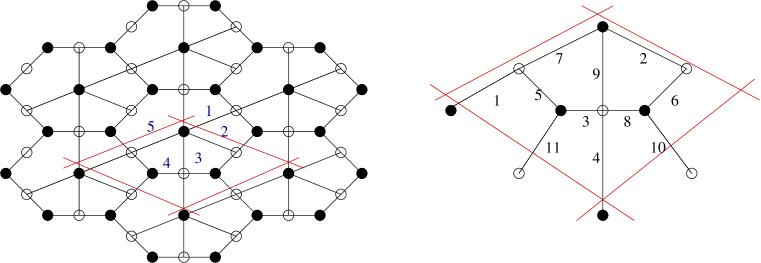
Figure 14: The dimer model and fundamental domain for the second del Pezzo surface is shown on the left. The blue integers label the faces. The fundamental domain and the labeling of the fields according to the superpotential in eq.(58) is shown on the right.

From fig. (14), we see that the faces in the dimer diagram are generated by the bifundamental fields

$$F1=\left(X_{1},X_{4},X_{8},X_{10}\right),~{}F2=\left(X_{1},X_{2},X_{5},X_{11}\right),~{}F3=\left(X_{2},X_{6},X_{8},X_{9}\right),$$ (60)

$$F4=\left(X_{3},X_{5},X_{7},X_{9}\right),~{}F5=\left(X_{3},X_{4},X_{6},X_{7},X_{10},X_{11}\right)$$

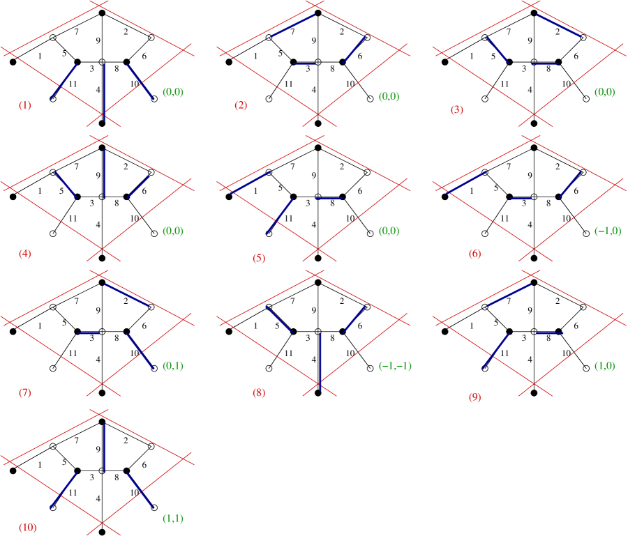
Figure 24: Perfect matchings corresponding to the model II of the $dP_{2}$ singularity, drawn from eq. (59). The perfect matching numbers are denoted by the red integers, while the green integers denote the height functions.

and these are, from eq. (59), given by the perfect matchings ${\tilde{p}}_{1}-{\tilde{p}}_{5}$, ${\tilde{p}}_{5}-{\tilde{p}}_{3}$, ${\tilde{p}}_{3}-{\tilde{p}}_{4}$, ${\tilde{p}}_{4}-{\tilde{p}}_{2}$, ${\tilde{p}}_{2}-{\tilde{p}}_{1}$ Hence, we need to check that the perfect matchings ${\tilde{p}}_{i},i=1,\cdots 5$ are now the internal matchings. In fig. (24) in the appendix, we have provided the ten perfect matchings of this theory as follows from eq. (59). From the height functions provided in the figure, we see that ${\tilde{p}}_{1},\cdots{\tilde{p}}_{5}$ are indeed the internal perfect matchings of the theory. The height functions also reproduce the correct multiplicities in the toric diagram of the second phase of $dP_{2}$ [26].

Let us summarise the discussion in this section. Here, we have implemented the inverse algorithm of [15], starting from the matching matrix of the parent orbifolds of the form $\mathbb{C}^{3}/\mathbb{Z}_{m}\times\mathbb{Z}_{n}$, with $(m,n)=(2,2)$, $(2,3)$ and $(3,3)$. This approach gives us a way of directly handling the vevs of the bifundamental fields in this theory. We have worked out several examples, some of which involved adjoint fields, which we have seen how to handle in the language of dimer models, by looking at the consistency of the matching matrix of the daughter singularities. We have, in two examples, checked our conjecture 2 stated in section 2. We have also seen how to rule out unphysical toric theories, apart from an apparent puzzle that we mentioned in subsection 4.2. These are the main results of this section.

5 Discussions

In this paper, we have performed a detailed analysis of certain aspects of dimer models corresponding to abelian orbifold singularities in string theory. To begin with, we discussed cyclic orbifolds, and studied the same using a combination of open and closed string techniques. In particular, we addressed the issues of symmetries of dimer models from a closed string perspective. Further, we have performed detailed analysis of Higgsing of non cyclic orbifolds of $\mathbb{C}^{3}$, including the simplest case where the orbifolding action is asymmetric. We have seen how the dimer model naturally incorporates the adjoint fields which typically arise in these cases. Clearly, these methods will be applicable to any abelian orbifold singularity, although the explicit computation of the perfect matchings become prohibitively difficult after the first few simple cases. The method of writing the perfect matchings from the Kasteleyn matrix is helpful in these situations. Using this, we have verified the two conjectures that we stated in section (2) for the orbifold $\mathbb{C}^{3}/\mathbb{Z}_{3}\times\mathbb{Z}_{5}$ although the results are too long to present here. The methods discussed in this paper illustrate the general inverse procedure involving dimers, for orbifold theories. As a future application of these results, it would be interesting to understand how (a possible variant of) dimer models capture the combinatorics of non-supersymmetric orbifolds which have localised closed string tachyons in their spectrum. In those situations, one typically deals with the case where $\alpha^{\prime}$ corrections are very small, i.e one is restriced to the classical moduli space of the gauge theory that lives on the world volume of the D-brane probing the orbifold. It can be checked that for such orbifolds the main concepts of dimer models break down, and that one needs a possible generalisation of the latter. As is known, such non-supersymmetric orbifolds exhibit flow properties (analogous to RG flows) to lower rank orbifolds, and it would be interesting to understand this dynamics from the standpoint of graph theory. Further, in the case of supersymmetric orbifolds, it would be interesting to explicitly prove our conjecture that in the case of generic toric varieties, the face symmetries of the corresponding dimer model involve only internal points in the toric diagram, whenever these are present.

Acknowledgments

We would like to sincerely thank Ami Hanany and Yang-Hui He for helpful email correspondence. We would also like to thank Ajay Singh for computer related help.

6 Appendix

In this appendix, we provide some of the details of our calculations that have not been provided in the main text.

We start with the singularity $\mathbb{C}^{3}/\mathbb{Z}_{5}$. This orbifold has two twisted sectors, as mentioned in the main text, with twisted sector R-charges $\left(\frac{1}{5},\frac{1}{5},\frac{3}{5}\right)$ and $\left(\frac{2}{5},\frac{2}{5},\frac{1}{5}\right)$. The ten perfect matchings for this orbifold, whose dimer covering is given in fig. (3) is shown in the fig. (15).

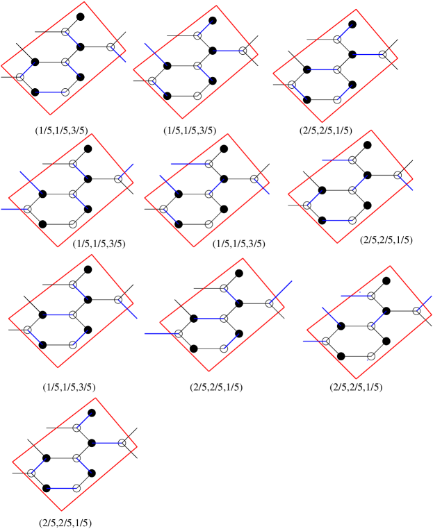
Figure 15: The ten perfect matchings for the orbifold $\mathbb{C}^{3}/\mathbb{Z}_{5}$

For the singularity $\mathbb{C}^{3}/\mathbb{Z}_{2}\times\mathbb{Z}_{3}$, the fundamental region and matching matrix are shown below. The perfect matchings for this orbifold are shown next. For reference, we have also indicated the height functions along with each matching.

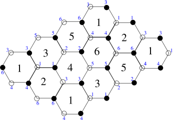
Figure 16: The fundamental region for the dimer covering of the orbifold $\mathbb{C}^{3}/\mathbb{Z}_{2}\times\mathbb{Z}_{3}$. We have used slightly different labeling conventions compared to what appears in the main text.

$${\cal M}=\pmatrix{~{}&p_{1}&p_{2}&p_{3}&p_{4}&p_{5}&p_{6}&p_{7}&p_{8}&p_{9}&p_{10}&p_{11}&p_{12}&p_{13}&p_{14}&p_{15}&p_{16}&p_{17}\cr X_{1}&1&0&0&1&0&1&0&1&0&1&0&0&0&0&0&1&0\cr X_{2}&1&0&1&0&0&1&1&0&0&0&1&0&0&0&1&0&0\cr X_{3}&1&0&0&0&1&0&1&1&0&1&0&0&0&1&0&0&0\cr X_{4}&1&0&0&1&0&1&0&1&0&0&1&0&1&0&0&0&0\cr X_{5}&1&0&1&0&0&1&1&0&0&1&0&1&0&0&0&0&0\cr X_{6}&1&0&0&0&1&0&1&1&0&0&1&0&0&0&0&0&1\cr Y_{1}&0&1&1&1&0&1&0&0&0&0&0&0&0&0&1&1&0\cr Y_{2}&0&1&1&0&1&0&1&0&0&0&0&0&0&1&1&0&0\cr Y_{3}&0&1&0&1&1&0&0&1&0&0&0&0&1&1&0&0&0\cr Y_{4}&0&1&1&1&0&1&0&0&0&0&0&1&1&0&0&0&0\cr Y_{5}&0&1&1&0&1&0&1&0&0&0&0&1&0&0&0&0&1\cr Y_{6}&0&1&0&1&1&0&0&1&0&0&0&0&0&0&0&1&1\cr Z_{1}&0&0&0&0&0&0&0&0&1&1&0&0&0&1&1&1&0\cr Z_{2}&0&0&0&0&0&0&0&0&1&0&1&0&1&1&1&0&0\cr Z_{3}&0&0&0&0&0&0&0&0&1&1&0&1&1&1&0&0&0\cr Z_{4}&0&0&0&0&0&0&0&0&1&0&1&1&1&0&0&0&1\cr Z_{5}&0&0&0&0&0&0&0&0&1&1&0&1&0&0&0&1&1\cr Z_{6}&0&0&0&0&0&0&0&0&1&0&1&0&0&0&1&1&1\cr}$$ (61)

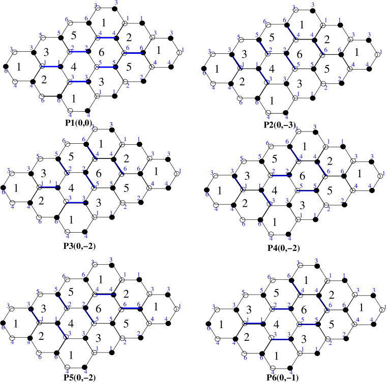
Figure 17: Perfect matchings for the orbifold $\mathbb{C}^{3}/\mathbb{Z}_{2}\times\mathbb{Z}_{3}$

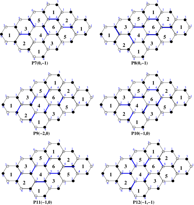
Figure 18: Perfect matchings for the orbifold $\mathbb{C}^{3}/\mathbb{Z}_{2}\times\mathbb{Z}_{3}$ (Contd.)

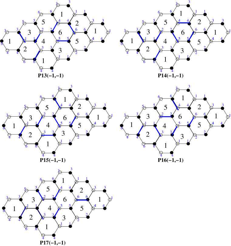
Figure 19: Perfect matchings for the orbifold $\mathbb{C}^{3}/\mathbb{Z}_{2}\times\mathbb{Z}_{3}$ (Contd.)

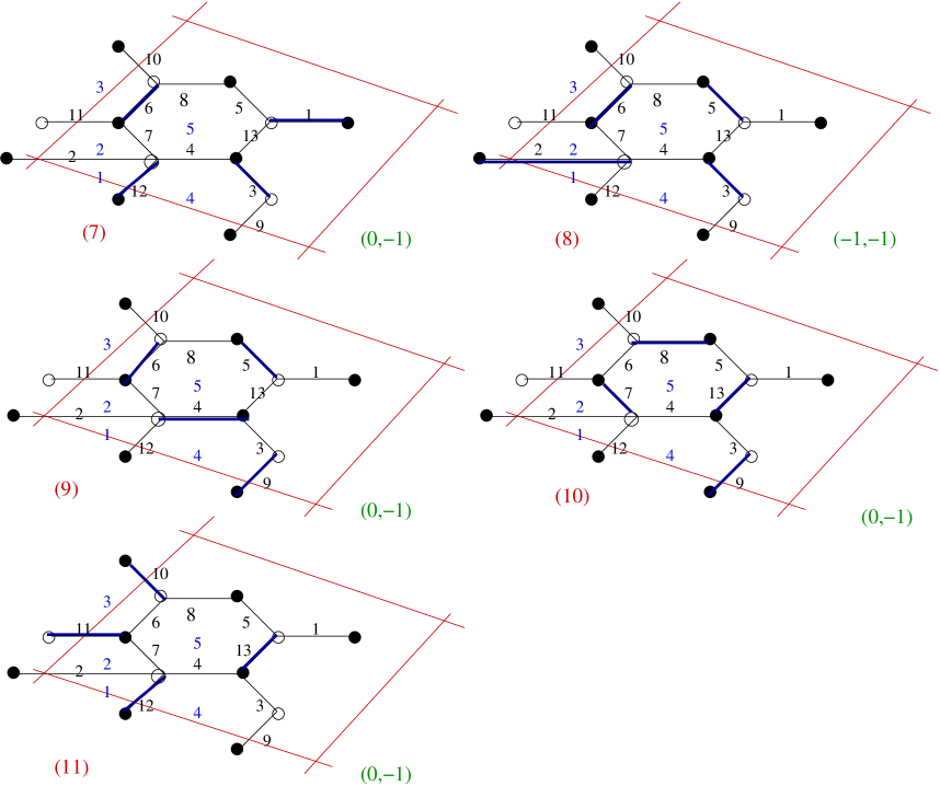
Figure 21: Continued : Perfect matchings for the orbifold $\mathbb{C}^{3}/\mathbb{Z}_{2}\times\mathbb{Z}_{3}$ with the field $X_{1}$ of eq. (61) removed. The same conventions as fig. (20) are followed.

For the orbifold $\mathbb{C}^{3}/\mathbb{Z}_{3}\times\mathbb{Z}_{3}$, the matching matrix is

$$\tiny{\left(\matrix{0&1&2&3&4&5&6&7&8&9&10&11&12&13&14&15&16&17&18&19&20&21&22&23&24&25&26\cr&&&&&&&&&&&27&28&29&30&31&32&33&34&35&36&37&38&39&40&41&42\cr X1&1&0&0&0&1&0&1&1&0&1&0&0&0&0&0&1&1&0&0&0&0&1&0&1&1&0\cr&&&&&&&&&&&0&0&0&1&1&0&0&0&0&0&0&1&0&0&1&0\cr X2&1&0&0&0&1&0&1&1&0&0&0&1&0&0&0&0&1&1&0&0&0&0&0&0&0&0\cr&&&&&&&&&&&0&0&0&0&0&0&0&0&0&1&1&1&1&1&1&1\cr X3&1&0&0&0&1&0&1&1&0&0&1&0&0&0&0&1&0&1&0&0&0&0&0&0&0&0\cr&&&&&&&&&&&0&0&0&1&1&1&1&0&1&0&1&0&0&1&0&0\cr X4&1&0&1&0&0&1&1&0&0&1&0&0&0&0&0&1&1&0&0&0&0&1&1&0&0&0\cr&&&&&&&&&&&0&0&1&0&0&0&0&1&0&1&0&1&1&0&0&0\cr X5&1&0&1&0&0&1&1&0&0&0&0&1&0&0&0&0&1&1&0&0&0&0&0&0&0\cr&&&&&&&&&&&1&0&1&0&0&1&1&0&0&1&1&0&0&0&0&0\cr X6&1&0&1&0&0&1&1&0&0&0&1&0&0&0&0&1&0&1&0&0&0&1&1&1&0&1\cr&&&&&&&&&&&0&1&0&1&0&1&0&0&0&0&0&0&0&0&0&0\cr X7&1&0&0&1&0&1&0&1&0&1&0&0&0&0&0&1&1&0&0&0&0&0&0&0&1&0\cr&&&&&&&&&&&1&0&1&0&1&0&1&1&1&0&0&0&0&0&0&0\cr X8&1&0&0&1&0&1&0&1&0&0&0&1&0&0&0&0&1&1&0&0&0&0&0&1&1&1\cr&&&&&&&&&&&1&1&0&0&0&0&0&0&0&0&0&0&0&0&1&1\cr X9&1&0&0&1&0&1&0&1&0&0&1&0&0&0&0&1&0&1&0&0&0&0&1&0&0&0\cr&&&&&&&&&&&0&1&0&0&0&0&0&1&1&0&0&0&1&1&0&1\cr Y1&0&0&0&0&0&0&0&0&1&1&0&1&1&0&1&0&1&0&0&1&0&1&0&1&1&1\cr&&&&&&&&&&&1&0&0&0&0&0&0&0&0&0&0&1&0&0&1&0\cr Y2&0&0&0&0&0&0&0&0&1&0&1&1&1&1&0&0&0&1&1&0&0&0&1&0&0&0\cr&&&&&&&&&&&0&1&0&0&0&0&0&0&0&1&1&0&1&1&0&1\cr Y3&0&0&0&0&0&0&0&0&1&1&1&0&0&1&1&1&0&0&0&0&1&0&0&0&0&0\cr&&&&&&&&&&&0&0&1&1&1&1&1&1&1&0&0&0&0&0&0&0\cr Y4&0&0&0&0&0&0&0&0&1&1&0&1&0&1&1&0&1&0&0&0&1&0&0&0&0&0\cr&&&&&&&&&&&0&0&1&0&0&0&0&1&0&1&0&1&1&0&1&1\cr Y5&0&0&0&0&0&0&0&0&1&0&1&1&1&0&1&0&0&1&0&1&0&0&0&0&0&1\cr&&&&&&&&&&&1&0&0&0&0&1&1&0&1&0&1&0&0&1&0&0\cr Y6&0&0&0&0&0&0&0&0&1&1&1&0&1&1&0&1&0&0&1&0&0&1&1&1&1&0\cr&&&&&&&&&&&0&1&0&1&1&0&0&0&0&0&0&0&0&0&0&0\cr Y7&0&0&0&0&0&0&0&0&1&1&0&1&1&1&0&0&1&0&1&0&0&0&0&0&1&0\cr&&&&&&&&&&&1&0&1&0&1&0&1&0&0&1&1&0&0&0&0&0\cr Y8&0&0&0&0&0&0&0&0&1&0&1&1&0&1&1&0&0&1&0&0&1&0&0&1&0&1\cr&&&&&&&&&&&0&1&0&1&0&1&0&0&0&0&0&0&0&0&1&1\cr Y9&0&0&0&0&0&0&0&0&1&1&1&0&1&0&1&1&0&0&0&1&0&1&1&0&0&0\cr&&&&&&&&&&&0&0&0&0&0&0&0&1&1&0&0&1&1&1&0&0\cr Z1&0&1&1&0&1&0&1&0&0&0&0&0&0&0&1&0&0&0&0&1&1&1&0&1&0&1\cr&&&&&&&&&&&0&0&0&1&0&1&0&0&0&0&0&1&0&0&1&0\cr Z2&0&1&1&0&1&0&1&0&0&0&0&0&1&0&0&0&0&0&1&1&0&1&1&0&0&0\cr&&&&&&&&&&&0&0&0&0&0&0&0&0&0&1&1&1&1&1&0&0\cr Z3&0&1&1&0&1&0&1&0&0&0&0&0&0&1&0&0&0&0&1&0&1&0&0&0&0&0\cr&&&&&&&&&&&0&0&1&1&1&1&1&0&0&1&1&0&0&0&0&0\cr Z4&0&1&1&1&0&1&0&0&0&0&0&0&0&1&0&0&0&0&1&0&1&0&1&0&0&0\cr&&&&&&&&&&&0&1&1&0&0&0&0&1&0&1&0&0&1&0&0&1\cr Z5&0&1&1&1&0&1&0&0&0&0&0&0&0&0&1&0&0&0&0&1&1&0&0&0&0&1\cr&&&&&&&&&&&1&0&1&0&0&1&1&1&1&0&0&0&0&0&0&0\cr Z6&0&1&1&1&0&1&0&0&0&0&0&0&1&0&0&0&0&0&1&1&0&1&1&1&1&1\cr&&&&&&&&&&&1&1&0&0&0&0&0&0&0&0&0&0&0&0&0&0\cr Z7&0&1&0&1&1&0&0&1&0&0&0&0&1&0&0&0&0&0&1&1&0&0&0&0&1&0\cr&&&&&&&&&&&1&0&0&0&1&0&1&0&1&0&1&0&0&1&0&0\cr Z8&0&1&0&1&1&0&0&1&0&0&0&0&0&1&0&0&0&0&1&0&1&0&0&1&1&0\cr&&&&&&&&&&&0&1&0&1&1&0&0&0&0&0&0&0&0&0&1&1\cr Z9&0&1&0&1&1&0&0&1&0&0&0&0&0&0&1&0&0&0&0&1&1&0&0&0&0&0\cr&&&&&&&&&&&0&0&0&0&0&0&0&1&1&0&0&1&1&1&1&1}\right)}$$

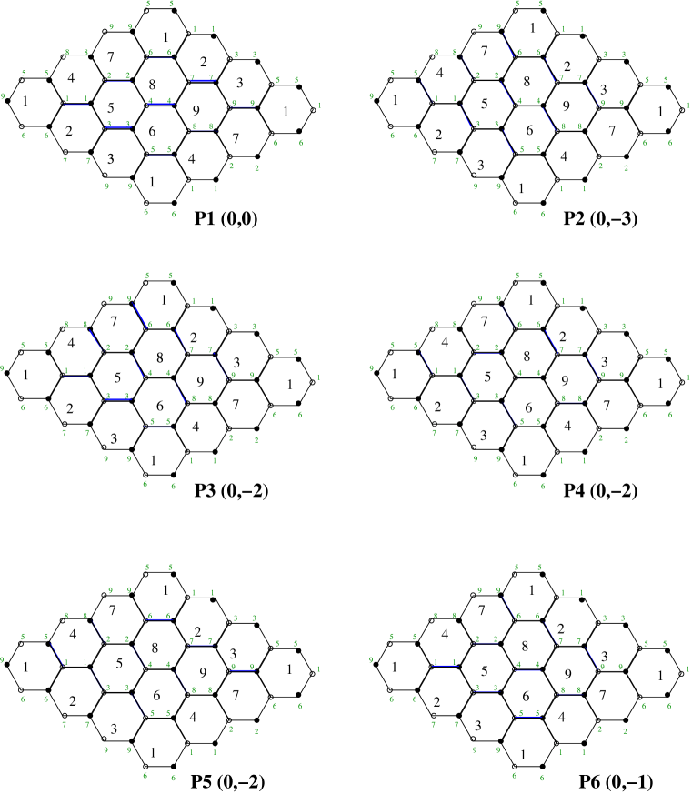
Figure 22: Some of the perfect matchings corresponding to the points on the edges of the toric diagram for the orbifold $\mathbb{C}^{3}/\mathbb{Z}_{3}\times\mathbb{Z}_{3}$. The corresponding height functions are given for reference. The closed string twisted sector R-charges can be read off by assigning weights $\left(\frac{1}{9},0,0\right)$, $\left(0,\frac{1}{9},0\right)$ and $\left(0,0,\frac{1}{9}\right)$ to the three types of edges.

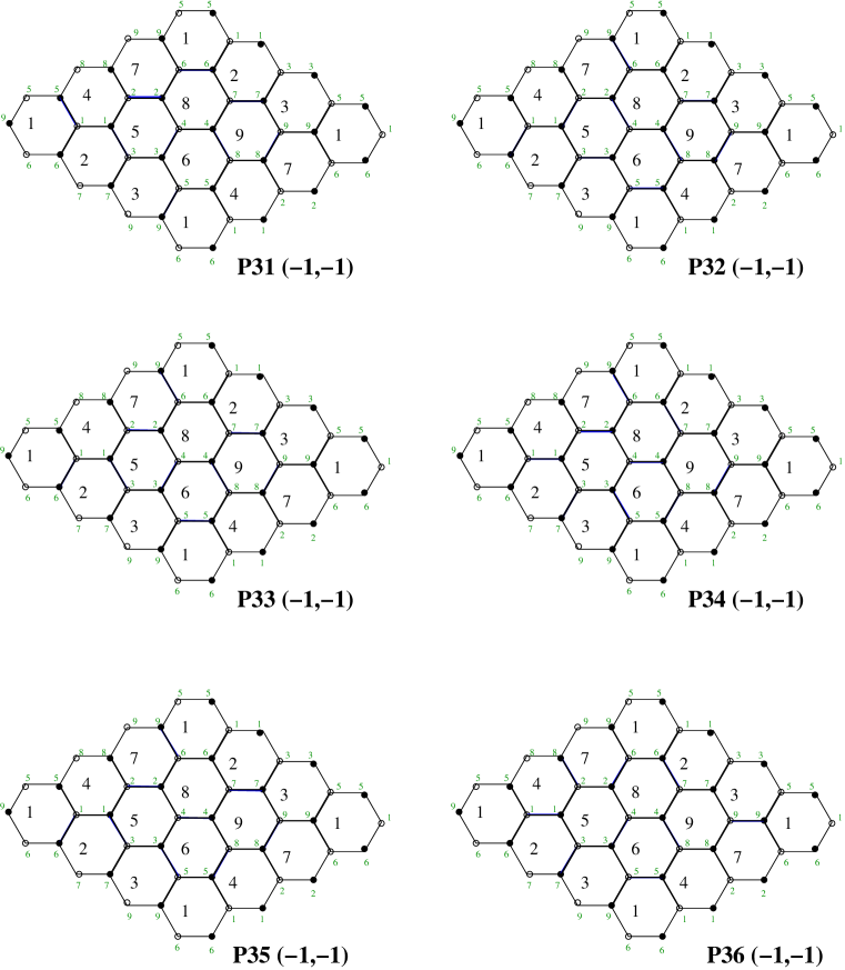
Figure 23: Some perfect matchings corresponding to the internal points in the toric diagram of the orbifold $\mathbb{C}^{3}/\mathbb{Z}_{3}\times\mathbb{Z}_{3}$

References

- [1] M. Cvetic, H. Lu, D. N. Page, C. N. Pope, “New Einstein-Sasaki spaces in five and higher dimensions,” Phys. Rev. Lett. 95 071101 (2005), hep-th/0504225
- [2] D. Martelli, J. Sparks, “Toric Sasaki-Einstein metrics on and ,” Phys. Lett. B 621, 208 (2005), hep-th/0505027
- [3] M. R. Douglas, G. W. Moore, “D-branes, quivers, and ALE instantons,” hep-th/9603167
- [4] M. R. Douglas, B. R. Greene, D. R. Morrison, “Orbifold resolution by D-branes,” Nucl. Phys. B506 (1997) 84, hep-th/9704151
- [5] D. Martelli, J. Sparks, “Toric geometry, Sasaki-Einstein manifolds and a new infinite class of AdS/CFT duals,” Comm. Math. Phys. 262 (2006) 51, hep-th/0411238
- [6] S. Benvenuti, S. Franco, A. Hanany, D. Martelli, J. Sparks, “An Infinite family of superconformal quiver gauge theories with Sasaki-Einstein duals,” JHEP 0506 (2005) 064, hep-th/0411264
- [7] P. Kasteleyn, “Graph theory and crystal physics,” in Graph theory and theoretical physics, pp 43 - 110, Academic Press, London, 1967.
- [8] R. Kenyon, “An introduction to the dimer model,” math.CO/0310236
- [9] A. Hanany, K. D. Kennaway, “Dimer models and toric diagrams,” hep-th/0503149
- [10] S. Franco, A. Hanany, K. D. Kennaway, D. Vegh, B. Wecht, “Brane dimers and quiver gauge theories,” JHEP 0601 2006, 096, hep-th/0504110
- [11] K. D. Kennaway, “Brane Tilings,” Int. J. Mod. Phys. A22 2007, 2977, arXiv:0706.1660 [hep-th]
- [12] M. Yamazaki, “Brane Tilings and Their Applications,” arXiv:0803.4474 [hep-th]
- [13] D. Forcella, A. Hanany, Y-H. He, A. Zaffaroni, “The Master Space of N=1 Gauge Theories,” arXiv:0801.1585 [hep-th]
- [14] T. Sarkar, “On Dimer Models and Closed String Theories,” JHEP 0710 2007 010, arXiv:0705.3575 [hep-th]
- [15] B. Feng, A. Hanany, Y-H He, “ D-brane gauge theories from toric singularities and toric duality,” Nucl. Phys. B595 (2001) 165, hep-th/0003085
- [16] C. Beasley, B. R. Greene, C.I. Lazaroiu, M. R. Plesser, “ D3-branes on partial resolutions of Abelian quotient singularities of Calabi-Yau threefolds,” Nucl. Phys. B566 2000, 599, hep-th/9907186
- [17] D. R. Morrison, M. R. Plesser, “Nonspherical Horizons 1,” Adv. Theor. Math. Phys. 3, 1999, 1, hep-th/9810201
- [18] S. Franco, D. Vegh, “Moduli spaces of gauge theories from dimer models : Proof of the correspondence,” JHEP 0611 (2006) 054, hep-th/0601063
- [19] J. Park, R. Rabadan, A. M. Uranga, “Orientifolding the conifold,” Nucl. Phys. B570 2000 38, hep-th/9907086
- [20] T. Sarkar, “ On localized tachyon condensation in and ,” Nucl. Phys. B700 (2004) 490, hep-th/0407070
- [21] E. Witten, “Phases of N=2 Theories in Two Dimensions,” Nuclear Physics B 403, (1993) 159, hep-th/9301042.
- [22] I. Garcia-Etxebarria, F. Saad, A. M. Uranga, “Quiver gauge theories at resolved and deformed singularities using dimers,” JHEP 0606 (2006) 055, hep-th/0603108
- [23] T. Muto, “D-branes on orbifolds and topology change,” Nucl. Phys. B521 (1998) 183, hep-th/9711090
- [24] T. Sarkar, “ D-brane gauge theories from toric singularities of the form and ,” Nucl. Phys. B595 (2001) 201, hep-th/0005166
- [25] B. Feng, S. Franco, A. Hanany, Y-H. He, “UnHiggsing the del Pezzo,” JHEP 0308 (2003) 058, hep-th/0209228
- [26] B. Feng, S. Franco, A. Hanany, Y-H. He, “Symmetries of toric duality,” JHEP 076 (2002) 0212, hep-th/0205144