The S1 Shell and Interstellar Magnetic Field and Gas near the Heliosphere

Abstract

Many studies of the Loop I magnetic superbubble place the Sun at the edges of the bubble. One recent study models the polarized radio continuum of Loop I as two magnetic shells with the Sun embedded in the rim of the ’S1’ shell. If the Sun is in such a shell, it should be apparent in both the local interstellar magnetic field and the distribution of nearby interstellar material. The properties of these subshells are compared to the interstellar magnetic field (ISMF) and the distribution of interstellar Fe⁺ and Ca⁺ within $\sim 55$ pc of the Sun. Although the results are not conclusive, the ISMF direction obtained from polarized stars within $\sim 30$ pc is consistent with the ISMF direction of the S1 shell. The distribution of nearby interstellar Fe⁺ with log $N$(Fe⁺)$<12.5$ cm^-2 is described equally well by a uniform distribution or an origin in spherical shell-like features. Higher column densities of Fe⁺ (log $N$(Fe⁺)$>12.5$ cm^-2) tend to be better described by the pathlength of the sightline through the S1 and S2 subshells. Column densities of the recombinant ion Ca⁺ are found to increase with the strength of the interstellar radiation field, rather than with star distance or total pathlength through the two magnetic subshells. The ion Ca⁺ can not be used to trace the distribution of local interstellar gas unless the spatial variations in the radiation field are included in the calculation of the ionization balance, in addition to possible abundance variations. The result is that a model of Loop I as composed of two spherical magnetic subshells remains a viable description of the distribution of nearby low density ISM, but is not yet proven.

1 Introduction

The location of the Sun in the rim of the Loop I superbubble has been inferred from radio continuum data, kinematical data on the flow of local ISM away from the center of Loop I, data on gas-phase abundances in local ISM, and the coincidence of the velocity of ISM inside and outside of the heliosphere. Loop I is an evolved superbubble shell formed from stellar evolution in a subgroup of the Sco-Cen association, $\sim 4-5$ Myrs ago (e.g. de Geus, 1992; Frisch, 1995, 1996; Maíz-Apellániz, 2001). Both the original dimensions found for the Loop I bubble observed in 820 MHz (Berkhuijsen, 1973), and more recent studies of Heiles (1998a, b, H98a,H98b) and Wolleben (2007), place the Sun in or adjacent to the rim of a magnetic superbubble shell for an assumed spherical geometry. The 1.4 GHz Wolleben study defines two magnetic subshells of Loop I, S1 and S2, with magnetic pole directions differing by $90^{\circ}\pm 42^{\circ}$. Comparisons between the radio continuum filaments of Loop I and optical polarization data indicate that the radio filaments at distances of $\sim 100-150$ pc trace magnetic field lines, indicating that optical polarization is a suitable tracer of magnetic shells (H98a). Both the kinematics and abundance pattern of local interstellar material (LISM) suggest that the Loop I remnant has expanded to the solar location (Frisch, 1981). LISM abundances of the refractory elements Mg, Fe, and Ca, show the characteristic enhancement indicative of grain destruction in interstellar shocks (Frisch et al., 1999). Local interstellar gas, $d<50$ pc, and dust flow away from the center of Loop I at a best-fit velocity of $\sim 18$ km s^-1 in the local standard of rest (LSR, e.g. Frisch et al., 2009). The first spectrum of backscattered Ly$\alpha$ emission from interstellar hydrogen inside of the heliosphere showed that the velocity of interstellar H^o inside of the heliosphere is comparable to LISM velocities (Adams & Frisch, 1977). Together these data suggest that the magnetic field and spatial configuration of the LISM can be used to test whether the Loop I magnetic superbubble has expanded to the solar location. The Wolleben (2007) model of the S1 and S2 shells provides enough detail to make preliminary comparisons between LISM data and the properties of these shells. These comparisons provide interesting insights into the LISM properties, and support the possibility that local ISM within $\sim 55$ pc is dominated by the S1 and S2 shells.

Superbubble expansion into ambient ISM with equal magnetic and thermal pressures yields roughly spherical superbubbles during early expansions stages when magnetic pressure is weak compared to the ram pressure of the expanding gas (MacLow & McCray, 1988; Ferriere et al., 1991), and bubbles elongated along the ISMF during late stages of evolution (Hanayama & Tomisaka, 2006). The evolved shell is thicker near the ISMF equatorial regions, where field strengths are larger due to flux freezing, than the polar regions of the shell where thermal pressure provides the main support for the shell. In media where magnetic pressure is weak, e.g. the ratio of thermal to magnetic pressure $\beta>10$, the evolved bubble is more symmetric. Supernovae in Sco-Cen Association subgroups have contributed to the evolution of the Loop I superbubble during the past $\leq 14$ Myrs. The Loop I superbubble (and S1, S2) expanded in a medium with a density gradient, because the initial supernova occurred in the molecular regions of the parent Scorpius-Centaurus Association subgroups, while the subsequent bubble expansion occurred in the low density interior of the Local Bubble cavity (Frisch, 1981, 1995; Fuchs et al., 2006). In this case the external plasma $\beta$ may have varied irregularly across the expanding shell, so that the topology of the present day S1 and S2 shells may deviate from axial symmetry as well as sphericity.

The ISMF direction at the heliosphere provides the most direct measure of whether the Sun is embedded in the shell of the Loop I superbubble. Several phenomena trace the field direction – the weak polarization of light from nearby stars (Tinbergen, 1982; Frisch, 2007a, hereafter F07), the flield direction in the S1 subshell of Loop I (Wolleben, 2007), the 3 kHz emissions from the outer heliosheath detected by the two Voyager satellites (Gurnett et al., 2006, F07), the observed angular offset between interstellar H^o and He^o flowing into the heliosphere (Lallement et al., 2005; Pogorelov & Zank, 2006; Opher et al., 2007), and the 10 pc difference between the distances of the solar wind termination shock detected by the two Voyager satellites (e.g. Stone, 2008). The orientation of the plane midway between the hot and cold dipole moments of the cosmic microwave background is also within $\sim 15^{\circ}$ of the local ISMF direction (F07).

This paper searches for evidence that the S1 and S2 shells affect the distribution of nearby ISM within $\sim 55$ pc. The topology of the S1 and S2 shells is discussed in §2. Section 3 shows that the direction of the ISMF at the Sun is consistent with the ISMF direction in the S1 shell, similar to the location of the mid-plane between the cosmic microwave dipole moments, and consistent with the ISMF direction inferred from heliosphere models. The distribution of the ISM in the S1 and S2 shells are compared to Fe⁺ column densities towards nearby stars behind the shells (§4). A similar comparison is made between the Ca⁺ data and the S1 and S2 shells, however Ca⁺ column densities appear instead to trace the strength of the local far ultraviolet (UV) diffuse radiation field (§5). An appendix outlines the ionization equilibrium of Ca⁺.

2 Approximating the Three-Dimensional ISM Distribution in the S1 and S2 Shells

Wolleben (2007) has fit two separate spherical magnetic shells (’S1’ and ’S2’) to the low frequency (1.4 GHz and 23 GHz) polarized radio continuum, which must have a relatively local origin because of the $\lambda^{2}$ dependence of Faraday rotation. The ISMF is assumed to be entrained in the expanding superbubble shell, with no deviation from spherical symmetry. The Sun is located in the rim of the S1 shell, which is centered $78\pm 10$ pc away at galactic coordinates $\ell,b=346^{\circ}\pm 5^{\circ},3^{\circ}\pm 5^{\circ}$. The upwind direction of the flow of local ISM past the Sun is within $\sim 20^{\circ}$ of of the S1 shell center. The inner and outer radii of the S1 shell are $72\pm 10$ and $91\pm 10$ pc respectively. Wolleben described the S1 magnetic field direction by two angles, the angle between the field direction and the NGP $\mathrm{B}_{\phi}$$=-72^{\circ}\pm 30^{\circ}$, and the rotation about the NGP $\mathrm{B}_{\theta}$$=71^{\circ}\pm 30^{\circ}$. The S2 shell center is more distant ($\sim 95$ pc) and centered at higher galactic latitudes ($b\sim 37^{\circ}$) than the S1 shell, with an ISMF direction near the north galactic pole. An alternate single-shell model for Loop I is also based on the H^o shell and centers the feature at $\ell$,$b$$=320^{\circ},5^{\circ}$ (H98a). As a first approximation of shell structure, they are assumed spherically symmetric, although the ISMF is seen in filaments interacting with denser clouds for more distant regions of Loop I (H98a) A more detailed model of these evolved bubbles requires understanding the magnetic pressure. The parameters provided for the S1 and S2 shells by Wolleben are detailed enough for comparison with observations of the LISM.

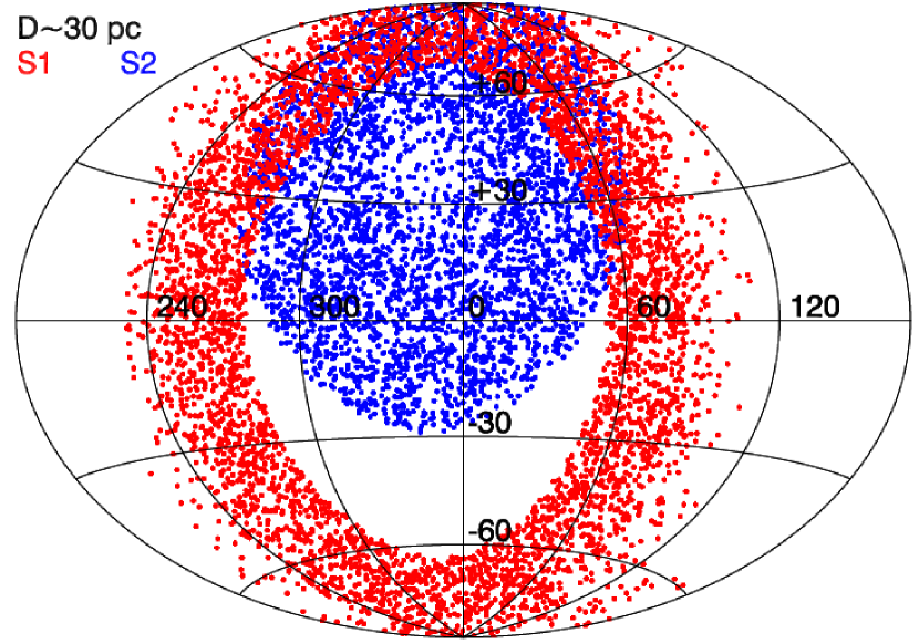
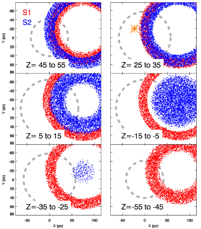
Figure 1: Left: The parts of the S1 and S2 shells about 30 pc from the Sun. Right: Distribution of points in the S1 (red) and S2 (blue) shells for different distance intervals Z (pc) above and below the galactic plane. The galactic center is at y=0 and x=infinity, beyond the plot right. The direction of galactic rotation is at x=0, y=infinity, beyond the plot bottom. The individual points trace the range of ISM distributions in the shells calculated with the assumption that each shell is spherically symmetric, and that the ISM is uniformly distributed. The dotted gray lines show the distance corresponding to 55 pc from the Sun for the midpoint of the Z-interval. The S1 shell distribution is for a shell centered at $\ell$,$b$$=346^{\circ},3^{\circ}$ and 78 pc, with a radius of 82 pc, and with a total rim thickness of 19 pc. The S2 shell distribution is for a shell centered at $\ell$,$b$$=347^{\circ},37^{\circ}$ and a distance of 95 pc, with a radius of 75 pc and total rim thickness of 24 pc. The orange star shows the location of the nearby cold filament towards Leo (Meyer, 2007; Lauroesch, 2007).

A three-dimensional (3D) spherically symmetric model of the S1 and S2 shells is created for comparison with the local interstellar magnetic field and distribution of interstellar Fe⁺ and Ca⁺. The 3D configuration is initially constructed in the frame of each shell such that the north pole is at the local zenith. The shell rims are filled with a uniform density of points. The shell model is then rotated to the galactic coordinate system by $\mathrm{B}_{\theta}$ and $\mathrm{B}_{\phi}$, and translated to the shell center in the galactic coordinate system. The result is a model where a path through the shell measures the shell column density normalized to an arbitrary value, and the shell column density in any sightline varies according to the end point of the path. Fig. 1, right, shows the ISM distribution in the S1 and S2 shells for slices parallel to the galactic plane and for 10 pc-wide intervals of Z above and below the galactic plane. Fig. 1, left, shows sections of the two shells at distances of $\sim 30$ pc using an aitoff projection. Negative Z-values are dominated by the S1 shell (red), below Z$\sim 30$ pc (latitudes $b\sim 20^{\circ}$). At higher latitudes a given sightline may sample either, or both, of the shells. The parameters of the 3D simulation place the Sun in the rim of the S1 shell, but the uncertainties quoted by Wolleben also allow the Sun to be in the S2 shell. As additional data on nearby ISM become available, it should become possible to both constrain and test the S1/S2 models in more detail.

The S1 and S2 shells overlap in places. One example is the sightline towards the stars $\alpha$ Oph (HD 159561), located 14.3 pc away at $\ell$,$b$$=35.9^{\circ},22.6^{\circ}$, which has the strongest Ca⁺ line observed towards any nearby star (Crawford, 2001). The S1 and S2 shells coincide at a distance of 12 pc in this sightline, suggesting that the Ca⁺ line towards $\alpha$ Oph samples a region where the S2 shell collided with the S1 shell, possibly creating a shock so that recent grain destruction occurred. Merging flows induce thermal instabilities that generate such filamentary structures (Audit & Hennebelle, 2005), and the more distant H^o gas in this sightline is also filamentary. A second example of possible interacting shells is the nearby Leo filament (Lauroesch, 2007). The orange symbol in Fig. 1 (Z=25–35 pc) shows the location of a tiny cold (20 K) filamentary ($>7^{\circ}\times 2^{\circ}$) cloud in Leo, located at $\ell$,$b$$=220^{\circ},45^{\circ}$ and at a distance of less than 42 pc (Meyer, 2007; Lauroesch, 2007). If the cloud is at 40 pc, it is outside of both shells for the basic values for the shell distances and radii (i.e. without invoking any uncertainties). However if the cloud is nearby, or if the extreme values allowed by the uncertainties on the S1 and S2 shells are invoked, this filament may form where the two shells collide. Merging flows induce thermal instabilities that generate such filamentary structures as the Leo filament (Lauroesch, 2007; Audit & Hennebelle, 2005), so the presence of this cold filament is consistent with the picture of the LISM as dominated by two shell features.

3 The S1 and S2 Shells and Local Interstellar Magnetic Field

3.1 S1 Shell and ISMF Direction

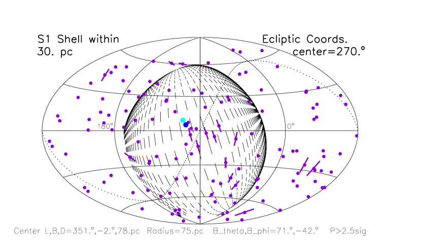
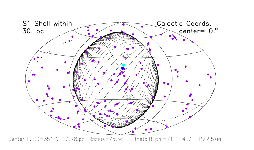
Figure 2: The magnetic field associated with the parts of the S1 shell within 30 pc is plotted in ecliptic coordinates (left) and galactic coordinates (right) for an aitoff projection. The ecliptic plot is centered at $\lambda=270^{\circ}$, while the galactic plot is centered at $\ell$=0^o. The parameters for the S1 shell given in Wolleben (2007) have been varied within the range of allowed uncertainties to yield the best match to the Tinbergen (1982) polarization data towards stars in the heliosphere nose region. The dark and light blue dots show the inflow directions of interstellar H^o and He^o into the heliosphere. The S1 subshell parameters used in the above figures correspond to a shell center at ($\ell$,$b$)=$(351^{\circ},-2^{\circ})$ and 78 pc, shell radius of 75 pc, and magnetic field angles $\mathrm{B}_{\theta}$=71^o, $\mathrm{B}_{\phi}$=–42^o. The dots show stars within 50 pc with polarization data, and the red bars show polarization vectors for stars where $P_{5}$$>2.5\sigma$ (Tinbergen, 1982; Piirola, 1977; Frisch, 2007a). The longitude increases towards the right for both figures.

Polarization by charged irregularly shaped interstellar grains yields polarization vectors that are parallel to the ISMF, because the induced magnetic torques naturally align the grains (e.g. Lazarian, 2000). There is a patch of dust towards the fourth galactic quadrant ($\ell$$>270^{\circ}$), mainly in the southern hemisphere and in the upwind direction of the interstellar gas flowing through the heliosphere, where the ISMF within 5–40 pc of the Sun has been traced by very weak optical polarizations (Tinbergen, 1982). The Tinbergen data were acquired in the southern hemisphere during 1974, and northern hemisphere data during 1973 (J. Tinbergen, private communication). Tinbergen detected polarizations of $\gtrsim 0.017$%, with $1\sigma\sim 0.007$%, towards a few stars within 40 pc. Five of these stars are close to the ecliptic plane, and offset by up to $\lambda$$\leq 40^{\circ}$ from the heliosphere nose towards positive ecliptic longitudes (Frisch, 2005, 2007a). The mean position angles for the three stars near the nose with $P>3\sigma$, are PA_G=$33^{\circ}\pm 11^{\circ}$ in galactic coordinates, and PA_E=$-26^{\circ}\pm 11^{\circ}$ in ecliptic coordinates (Table 1). The position angle uncertainty is estimated by allowing Q and U to vary over $\pm 1\sigma$ (Table 1). The nearest star towards the nose is 36 Oph, at 6 pc, and it has a $2.5\sigma$ detection with $P=0.018$%. The polarization position angle of 36 Oph (PA_E=–19.9, PA_G=39.5) does not differ significantly from the mean position angle of the three more distant stars with $3\sigma$ polarizations in the nose region. The polarizations of the Tinbergen’s sample, together with northern hemisphere data of Piirola (1977), are plotted in Fig. 2. An alternative catalog of nearby star polarizations is the comprehensive catalog assembled by Leroy (1993); however it is mainly based on measurements with larger uncertainties, and is therefore less useful for identifying very low polarization levels.

In order to test the relation between the ISMF in the S1 shell and the Tinbergen polarization data, the ISMF direction for the S1 shell was varied within the uncertainties on $\mathrm{B}_{\theta}$ and $\mathrm{B}_{\phi}$ to find the direction that is the most consistent with the optical data. The best match to the optical polarization data was found for $\mathrm{B}_{\theta}$$=71^{\circ}$ and $\mathrm{B}_{\phi}$$=-42^{\circ}$. The parts of the S1 shell within 30 pc are compared to the optical polarization data in Fig. 2, for galactic (right) and ecliptic (left) coordinates, for stars within 50 pc; polarization vectors are plotted if $P>2.5\sigma$. For the purpose of this figure, I use a center position for the S1 shell of ($\ell$,$b$)$=(351^{\circ},-2^{\circ})$ and radius 75 pc, so that the Sun is located 3 pc outside of the shell rim. The mean position angle of the S1 magnetic field (for $\mathrm{B}_{\phi}$=–42^o) at the star locations is PA_S1,E$=-20\pm 5$ in ecliptic coordinates, which is within the uncertainties of the stellar polarizations. A slightly larger value of $\mathrm{B}_{\phi}$ exactly matches the mean position angles of the starlight polarizations, but violates the quoted uncertainties. Therefore, the ISMF directions from the Tinbergen data and S1 shell configuration are consistent to within the uncertainties.

The Tinbergen stars with the strongest polarizations are $\sim 90^{\circ}$ from the pole of the S1 shell, which is consistent with the expectation of higher ISMF field strengths where the shell expansion is perpendicular to the ISMF direction. The best value for the S1 magnetic field direction close to the Sun, derived from comparisons with these optical polarization data (§3), is $\mathrm{B}_{\theta}$$=71^{\circ}$ and $\mathrm{B}_{\phi}$$=-42^{\circ}$, corresponding to a local ISMF direction towards $\ell$,$b$$=71^{\circ},48^{\circ}$.

Heliospheric asymmetries are caused by interactions with the interstellar magnetic field. A widely used measure of the heliosphere distortion due to the ISMF, which is inclined by the angle $\alpha\sim 30^{\circ}-60^{\circ}$ with respect to the ISM flow vector, is the observed offset between the inflowing He^o and H^o directions (Witte, 2004; Lallement et al., 2005). The ISMF also shifts the maximum Ly$\alpha$ emission originating in the outer heliosheath (Ben-Jaffel et al., 2000). Correcting the He^o and H^o directions to a common observation epoch yields an offset angle separation of $4.9^{\circ}\pm 1^{\circ}$ between the two directions. (The upwind direction of the He^o flow in J2000 coordinates is $\lambda$$=255.4^{\circ}\pm 0.5^{\circ}$, $\beta$$=5.1^{\circ}\pm 0.2^{\circ}$, Witte, private communication). These directions define a position angle, which is PA_E$=-35^{\circ}\pm 20^{\circ}$ (PA_G$=26^{\circ}\pm 20^{\circ}$) in ecliptic (galactic) coordinates, respectively. Large uncertainties are quoted because the upwind direction of the H^o flow through the heliosphere is not precisely defined due to the $\sim 50$% of the interstellar H^o lost to filtration in the hydrogen wall, the balance between radiation pressure and gravity affecting trajectories of H^o atoms surviving to the heliosphere interior, and the production of secondary H^o atoms inside of the heliosphere (e.g., Quémerais & Izmodenov, 2002). For comparison, at the heliosphere nose location, $\ell$,$b$$=3.5^{\circ},15.2^{\circ}$, the S1 shell with $\mathrm{B}_{\phi}$=–42^o gives a position angle PA_E=$-15^{\circ}$. The position angle formed by the offset between He^o and H^o flowing through the heliosphere is marginally consistent with the S1 shell direction at the heliosphere nose. The 10 AU difference in the termination shock distance found by Voyagers 1 and 2, in 2004 and 2007 respectively (Stone, 2008), must be combined with the H^o-He^o offset to provide a more reliable constraint on models of the direction of the interstellar magnetic field affecting the heliosphere (e.g. Pogorelov et al., 2007; Opher et al., 2007).

3.2 S1 shell and the CMB Dipole Moment

The great circle that is midway between the hot and cold poles of the cosmic microwave background (CMB) dipole passes within $5^{\circ}$ of the interstellar He^o upwind direction, and bifurcates the heliosphere nose (Frisch, 2007a). The point of closest approach to the nose is at $\ell$,$b$$=7.4^{\circ},11.6^{\circ}$, where the position angle of the CMB dipole mid-plane in ecliptic coordinates is PA_E$=-11^{\circ}\pm 1^{\circ}$ (uncertainties in the upwind He^o direction, used to define the nose position, are included in this uncertainty, Table 1). For comparison, the S1 shell magnetic field direction at this location, for $\mathrm{B}_{\phi}$$=-42^{\circ}$, corresponds to a position angle (ecliptic coordinates) of PA_E=$-18^{\circ}$. This fact is mentioned here because the low-$\ell$ multipole moments of the CMB show symmetries related to the ecliptic geometry (e.g. Copi et al., 2006), so that the symmetry of the CMB dipole moment around the heliosphere nose should also be of interest. The upwind direction is $5^{\circ}$ above the ecliptic plane, so any coincidence between the CMB multipole moments and the ecliptic geometry is tantamount to a coincidence with the heliosphere morphology and/or to the interstellar magnetic field that shapes the heliosphere. These ecliptic signatures on the CMB are not understood, but it is not unreasonable to postulate they arise from processes related to the local interstellar magnetic field and its effect on the heliosphere.

4 Comparisons between S1 and S2 Shells and Distribution of Fe⁺ 

If the distribution of nearby ISM is determined by the S1 and S2 magnetic superbubbles, then the S1 and S2 shell morphologies should be imprinted on the strengths of interstellar absorption lines. Fig. 1 shows two views of the ISM associated with the S1 and S2 shells. Interstellar absorption lines towards stars within 55 pc show that most of the the LISM is warm, $\sim 3,000-12,000$ K (Redfield & Linsky, 2004) with low average spatial densities, $<0.1$ cm^-3. Exceptions are the tiny dense clouds occasionally seen in Na^∘ and H^o absorption (Meyer, 2007). Models of the radiative transfer properties of the circumheliospheric ISM show a partially ionized, low density cloud, $n$(H^∘)$\sim 0.20$ cm^-3, $n_{\mathrm{e}}$$\sim 0.07$ cm^-3, and with temperature $\sim 6,300$ K determined from interstellar He^o inside of the heliosphere (Witte, 2004; Slavin & Frisch, 2008, SF08). Therefore, a suitable tracer of the S1 and S2 shell morphologies should be abundant, insensitive to cloud ionization, and undepleted. There are no available data sets that meet all three requirements, therefore the criteria that the element be undepleted is dropped. The best element for this study is then Fe⁺, which has been measured towards $\sim 27$ stars within 56 pc (Lehner et al., 2003; Redfield & Linsky, 2002; Kruk et al., 2002). Iron is predominantly singly ionized in the cloud around the heliosphere, with neutral and Fe⁺⁺ together containing less than 3% of the Fe atoms (SF08). A more difficult aspect of using Fe⁺ to trace absolute ISM densities is the factor of $\sim 6-40$ difference in the gas-phase Fe⁺ abundances between dense cold and warm tenuous clouds, due to dust grain destruction by interstellar shocks including in local regions (e.g. Slavin et al., 2004). The alternative common element that traces both neutral and ionized gas is Mg⁺, however it has similar abundance variations as Fe⁺ and the Mg⁺ h and k lines may be more saturated than the Fe⁺ lines. Therefore, I use Fe⁺ column densities to trace the distribution of local ISM. Three nearby stars are omitted from this discussion because they have known debris disks (HD 215789, HD 209952, HD 216956, Su et al., 2006).

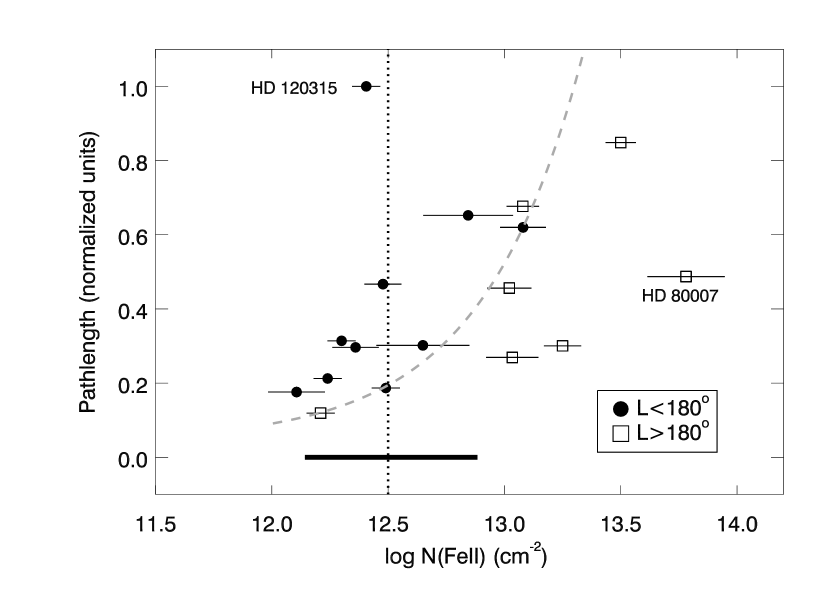
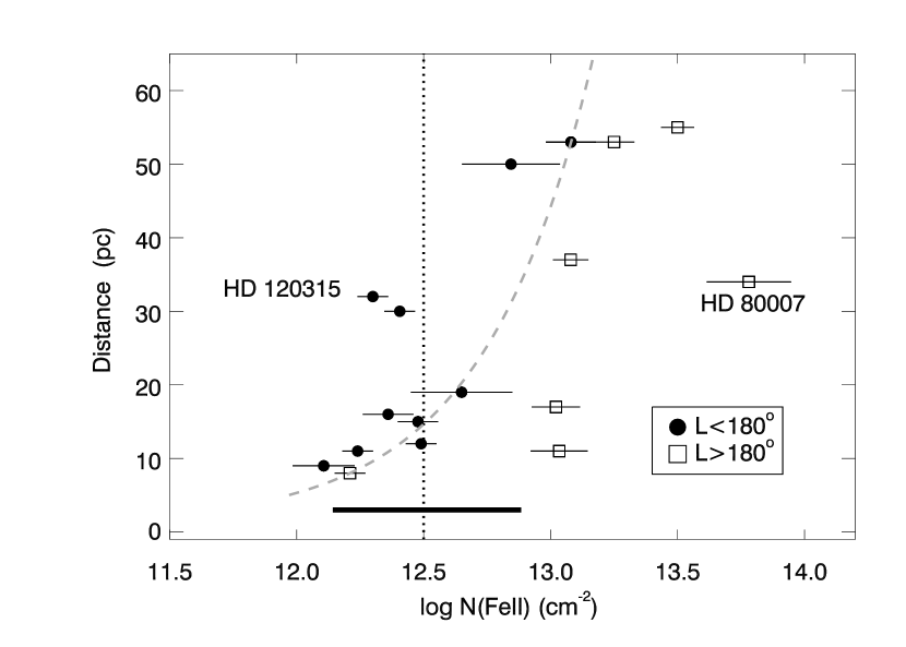
Figure 3: Column densities of Fe⁺ are plotted against the total predicted pathlength through the S1 and S2 shells foreground to the stars (or equivalently column densities, in arbitrary units) through the S1 and S2 shells (left, see §4) and against the star distance (right). The symbols indicate stars with stars 6–56 pc away and with galactic longitude $\ell$$>180^{\circ}$ (open squares) and $\ell$$<180^{\circ}$ (filled dots). The horizontal bar at the bottom shows the column density range for the stars within 6 pc that are not plotted. The vertical line separates stars with log $N$(Fe⁺)$<12.5$ cm^-2 versus $>12.5$ cm^-2  where column densities tend to increase with distance or pathlength through the shells, respectively. The stars are listed in Fig. 4. The dashed line shows a first order fit between the total column densities and pathlength (left), and total column densities and star distance (right). The individual velocity components for each star are added to give the total $N$(Fe⁺) plotted on the abscissa. The highest Fe⁺ column density in this sample is towards $\beta$ Car (HD 80007), 34 pc from the Sun in the direction $\ell$,$b$$=286^{\circ},-14^{\circ}$. According to Fig. 1, right, and Fig. 4, left, this star samples a tangential pathlength through the S1 shell.

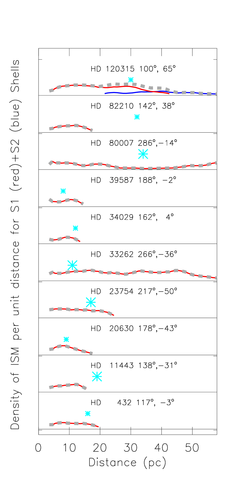
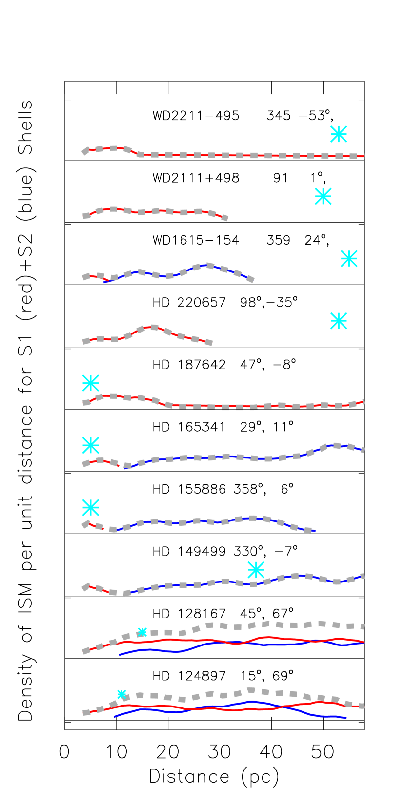
Figure 4: The distributions of ISM in the S1 shell (red) and S2 shell (blue) are shown towards each star in Fig. 3, based on a spherical morphology for each shell (see text). The distributions are plotted for arbitrary density units. The sum of the S1 and S2 densities is plotted as the thick gray dotted line. The turquoise symbol shows the distance of the star (labeled by name and coordinates), and small (large) symbol sizes show log $N$(Fe⁺)$<12.5$ cm^-2 ($>12.5$ cm^-2) towards the star.

Comparisons between log $N$(Fe⁺) and the column density of shell gas (S1 and S2) in front of each star, versus a comparison between $N$(Fe⁺) and the star distance, provide useful insights (Fig. 3). The shell column density towards each star represents the sum of the densities through the parts of the S1 and S2 shells foreground to the star, normalized to an arbitrary value. This pathlength was constructed by assuming a column width of $\pm 5$ pc in order to smooth out uncertainties in the intrinsic shell parameters (Table 1 in Wolleben, 2007). Because of this smoothing, stars within 6 pc are omitted from Fig. 3. The bar at the bottom of the figures shows the column density range for stars within 6 pc. For low column densities, log $N$(Fe⁺)$<12.5$ cm^-2, Fe⁺ column densities tend to increase with star distance. For higher column density sightlines, log $N$(Fe⁺)$>12.5$ cm^-2, $N$(Fe⁺) clusters more tightly around the shell pathlength (e.g. column density) than around the star distance. The exceptions to both comparisons are the stars HD 120315 (a low column density, high-latitude star that should sample a long pathlength through the shells) and HD 80007 (a high column density low-latitude star, with a path that is tangential to the S1 shell). The Fe⁺ components in a sightline are summed together for this comparison. The dashed lines in Fig. 3 show a linear fit between the column densities and the ordinate. The individual stars are listed in Fig. 4, where the relative column densities of the S1 and S2 shells towards each star are shown.

A second property of the distribution of Fe⁺ in these figures is that stars with galactic longitudes $>180^{\circ}$ tend to have larger Fe⁺ column densities, at a given distance, than stars in the opposite hemisphere. This effect is not seen in D^o or H^o. One possible reason is that the Fe abundances differ between the two hemispheres. The problem with this explanation is that it requires abundance variations over spatial scales of several parsecs, in relatively low velocity ISM ($<20$ km s^-1 LSR), with the variations ordered by the arbitrary coordinate of galactic longitude. An alternative explanation is that the Fe⁺ lines for $\ell$$<180^{\circ}$ include cool unresolved clumps of ISM. The ISRF towards $\ell$$>180^{\circ}$ is significantly larger than towards $\ell$$<180^{\circ}$ (§5), so that ISM for $\ell$$<180^{\circ}$ experiences reduced heating because of the absorption of H-ionizing photons, which may allow unresolved ISM clumps to coexist with warmer gas at the same velocity. Once the ionization of local ISM is better understood, the morphology of the S1 and S2 shells can be adjusted to better represent the actual distribution of the local ISM.

The stars within 6 pc show total column densities log $N$(Fe⁺)$=12.14-12.88$ cm^-2. Of these stars, the strongest lines are towards HD 155885, HD 165341, and HD 187642 in the upwind direction.

The distributions of S1 and S2 shell material towards each star are shown in Fig. 4. Stars with high (low) column densities are plotted as large (small) symbols for each direction. The most evident property is that the S1 shell dominates the ISM towards the southerly stars. These can be used to predict whether a star (or exoplanet system for example) will be embedded in a cloud-like feature or in the Local Bubble plasma. The assumed spherical morphology for S1 and S2 leads to the predictions that the white dwarf HD149499B (WD1634-573) is embedded in in the relatively denser gas of the shell, while the white dwarf WD1615-154 will be embedded in the low density Local Bubble plasma.

5 Ca⁺ and Electron Densities in the S1, S2 Shells

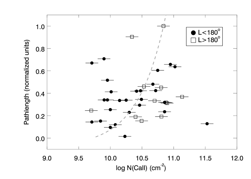
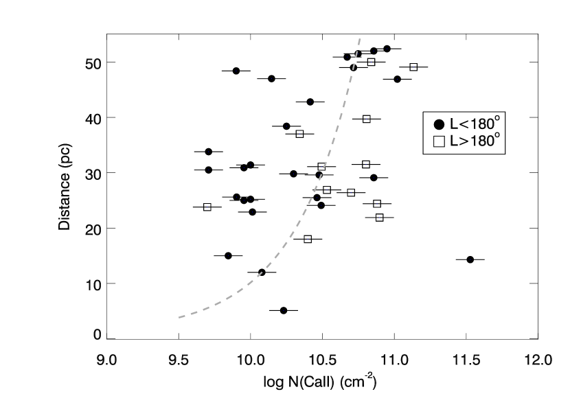
Figure 5: Left: Column densities of Ca⁺ are plotted against the total predicted pathlength (in arbitrary units) through the S1 and S2 shells sampled by each star. The stars are 5–55 pc away and are coded by whether the galactic longitude is $\ell$$>180^{\circ}$ (open squares) or $\ell$$<180^{\circ}$ (filled dots). The dotted line shows a first order fit between the total column densities and pathlength (left), and total column densities and star distance (right). The first two galactic quadrants, $\ell$$=0^{\circ}-180^{\circ}$ show generally smaller Ca⁺ column densities than do stars with $\ell$$=180^{\circ}-360^{\circ}$. The individual velocity components for each star are added to give the total $N$(Ca⁺) plotted on the absicissa. Right: The same set of stars are plotted against the distance of the star from the Sun.

Interstellar Ca⁺ is a recombinant species that traces the electron density as well as abundance variations. Because Ca⁺ is formed through recombination, it is a proxy for the electron density in nearby low density gas providing that abundance variations and the radiation field are understood. If the ISRF and electron densities are uniform throughout the S1 and S2 shells, then Ca⁺ column densities would show a similar dependence on pathlength through the shells as seen for Fe⁺. Interstellar Ca⁺ column densities are plotted against the pathlength through the S1 and S2 shells (Fig. 5, left) and star distance (Fig. 5, right), using data from (Frisch et al., 2008, 2002; Welty et al., 1996). The Ca⁺ column densities do not correlate with either the star distance or pathlength through the S1 and S2 shells. Sightlines where the Ca⁺ column density is an upper limit are not included in this comparison.

Higher Ca⁺ column densities are found for stars with $\ell$$>180^{\circ}$, as was seen for Fe⁺. The mean Ca⁺ column density is $\sim 40$% higher for stars in Quadrants III and IV, $\ell$$>180^{\circ}$, compared to stars with $\ell$$<180^{\circ}$. The difference becomes a factor of two if the anomalously strong Ca⁺ line towards $\alpha$ Oph is ignored. For $\ell$$<180^{\circ}$, $<$$N$(Ca⁺)$>=3.7\times 10^{10}$ cm^-2 (23 stars). Omitting $\alpha$ Oph, which has the strongest known Ca⁺ for nearby stars (e.g. Crawford, 2001), gives a mean for the $\ell$$<180^{\circ}$ sample of $<$$N$(Ca⁺)$>=2.3\times 10^{10}$. For $\ell$$>180^{\circ}$, $<$$N$(Ca⁺)$>=5.1\times 10^{10}$ cm^-2 (23 stars). No similar effect is seen in H^o (or D^o) column densities towards nearby stars (based on data in Wood et al., 2005). For stars within 50 pc, the mean H^o column density does not vary between the $\ell$$<180^{\circ}$ hemisphere and the $\ell$$>180^{\circ}$ hemisphere, and both show a mean value of $N$(H^∘)$\sim 1.5\times 10^{18}$ cm^-2 for respective sample sizes of 25 and 27 stars.

A different picture emerges when Ca⁺ (and Fe⁺) column densities are compared to the far UV radiation flux at the star. The highest diffuse far UV fluxes are seen towards stars in the third and fourth galactic quadrants, $\ell$$>180^{\circ}$, because of the low ISM opacity in the Local Bubble interior, hot stars in the Scorpius-Centaurus Association, and $\alpha$ Vir (Gondhalekar et al., 1980; Opal & Weller, 1984, Go80,OW84). Fluxes at 975 A are given for the 25 brightest stars, based on a survey by the $STP~{}72-1$ satellite in the 910–1050 A band and flux models (OW84). At least 97% of the local flux at 975 A is provided by the stars with $\ell$$>180^{\circ}$. Using the 975 A data for the 25 brightest stars (OW84), the 975 A flux was calculated at each star and is plotted against Ca⁺ column densities (Fig. 6, left), and Fe⁺ column densities (Fig. 6, right). The Fe⁺ and Ca⁺ samples are different, with more than half of the Fe⁺ stars within 20 pc, while most of the Ca⁺ stars are beyond 20 pc. All of the stars in the Fe⁺ data set with 975 A flux levels larger than $6.8\times 10^{4}$ photons cm^-2 s^-1 A^-1 are in galactic Quadrants III and IV, and these stars tend to have larger Fe⁺ column densities. The ISRF gradient would affect $N$(Fe⁺) only through larger column densities of HII, since Fe⁺ dominates in both ionized and neutral diffuse ISM. Nearby H II gas in regions with $\ell$$>180^{\circ}$ would explain Fe⁺variations, without violating the H^o constraints (which are determined from a similar star sample).

The dependence of Ca⁺ column densities on the 975 flux is less simple because Ca⁺ is a trace species formed by recombination, with an ionization potential of 11.87 eV versus 13.60 eV for H^o. In the cloud around the Sun, $n\sim 0.2$ cm^-3 and Ca⁺⁺/Ca⁺=63 (SF08). The ISRF gradient near the Sun (Fig. 6) affects $N$(Ca⁺) several ways. Higher radiation fluxes lead to higher electron densities, increasing Ca⁺⁺$\rightarrow$Ca⁺ recombination, and the overall H⁺ fraction would increase. Higher radiation fluxes also increase the Ca⁺ photoionization rate, but this effect does not appear to be dominant. In the local ISM, photoionization appears to dominate over collisional ionization. Radiative transfer models of the ISM surrounding the Sun match available ionization data such as the Mg⁺/Mg^∘ ratio (SF08). Low observed Ar^∘ abundances towards nearby stars also indicate the dominance of photoionization (Sofia & Jenkins, 1998). The radiation flux at 1044 A capable of ionizing Ca⁺ is traced by the 975 A radiation field, to within $\sim 10$% (Go80,OW84), so that Ca⁺ ionization rates should increase with the 975 flux. The increase of $N$(Ca⁺) with radiation flux is predicted by the photoionization equilibrium of Ca⁺ (see the appendix). Predicted $N$(Ca⁺) values are plotted against the ISRF for three different total H column densities, $N$(H)=$N$(H^∘)+$N$(H⁺), in Fig. 6. The observed increase of $N$(Ca⁺) with higher fluxes is consistent with Ca⁺ photoionization, and indicates that higher electron densities and H II column densities are both significant factors in the Ca⁺ line strengths.

6 Discussion and Conclusions

The discussions in this paper are based on a search for evidence of the S1 and S2 shells in local ISM data. The S1 and S2 shells are assumed to be spherical and complete. Such simple assumptions are justified only in the initial stage of probing the ISM distribution associated with a superbubble shell that has column densities too low for H^o 21-cm measurements, and that has evolved into a very low density region of space. Several studies model the formation of the Local Bubble in terms of the energy injected into the ISM by supernovae in the Sco-Centaurus Association (de Geus, 1992; Frisch, 1998; Maíz-Apellániz, 2001), but the connection between the Loop I radio emission and very local ISM has never been established. The S1 and S2 shell models provide a basis for testing this connection.

Early optical polarization data (Tinbergen, 1982) indicate that the ISMF direction close to the Sun agrees with the S1 shell ISMF direction once the uncertainties in Wolleben ’s $\mathrm{B}_{\phi}$ angle (2007) are included. In principle Fe⁺ can be used to trace the ISM distribution, since is arises in both neutral and ionized gas. Detailed comparisons between Fe⁺ line strengths towards nearby stars and the projected pathlength through the S1 and S2 shells towards that star support, but do not prove, that the lines arise in shells. Both the Fe⁺ and Ca⁺ data indicate that the portions of the S1 and S2 shells with $\ell$$>180^{\circ}$ will be more highly ionized than in the opposite hemisphere. The data are not sufficient to distinguish an ionization gradient from an abundance gradient. For this reason, the shells are better traced using ions with first ionization potentials less than 13.7 eV. Heating by Ly$\alpha$ radiation accounts for $\sim 66$% of the heating of the circumheliospheric ISM, so shell regions exposed to the highest radiation flux should also be warmer (an effect not explicitely included in the Ca equilibrium discussion in the appendix).

These models of the S1 and S2 shells assume spherically symmetric forms, which may be viable only for low density sightlines where magnetic and thermal pressures are comparable. Interstellar data are compared mainly to the S1 shell, which has the most favorable geometry for surrounding the Sun according to Wolleben (2007). The Tinbergen data suggest a slow increase in polarizations with distance, and the position angles towards the nose are consistent with the optical polarization of more distant stars in Loop I (Frisch, 2007a).

The most distant shell regions, in the galactic center hemisphere, have expanded into the high-extinction gas beyond $\sim 100$ pc that is associated with the Sco-Cen Association (see e.g. Figs. 1,3 in Chen et al. (1998) or Fig. 2 in Frisch (2007b)) and show pronounced magnetic filaments (H98a) rather than a spherical shell geometry. Heiles points out that the synchrotron-emission ridges of Loop I follow the distortion of the nearby global ISMF, as traced by polarization data, and that Loop I is not a shell for the high density regions. The global ISMF within several hundered parsecs is directed towards $\ell$$\sim 80^{\circ}-88^{\circ}$. The expansion of the nearest portions of the S1 shell in a uniform field would yield an ISMF close to the Sun directed upwards with respect to the galactic plane.

Hanayama & Tomisaka (2006) model the properties of a magnetic superbubble $\sim 3$ Myrs old and for the strong ISMF case, where magnetic pressure dominates thermal pressure by a factor of $\sim 2$. The superbubble cavity is elongated in the direction parallel to the ISMF, where the shell is thinner. The shell is thicker and more extended in the radial direction, $\sim 90^{\circ}$ from the magnetic pole. The region of strongest polarization for the Tinbergen sample is $\sim 90^{\circ}$ from the magnetic pole. Non-uniform shell expansion, or a ’wrinkled’ shell, could explain the anomalous sightlines towards HD 120315 and HD 80007 (see Fig. 3 compared to Fig. 4), while the tiny dense nearby Leo cloud (Meyer et al., 2006, Lauroesch private communication), and the exceptionally strong Ca⁺ line towards Rasalhague (HD 159561, $\alpha$ Oph) may indicate a region of merging shells.

The column densities for Fe⁺ and Ca⁺ are generally weaker for sightlines with $\ell$$<180^{\circ}$, and stronger for stars with $\ell$$>180^{\circ}$. This effect may be either from the distribution of ionized gas, or abundance variations for Fe and Ca. The effect is seen over small spatial scales of $\pm 10$ pc. If the variation is due to abundance differences, then the ISM close to the Sun would have two different histories, although the flow velocities are similar.

The conclusions of this comparison between the S1 and S2 shells with LISM markers can be briefly summarized:

• The Wolleben (2007) description of the Loop I polarized radio continuum in terms of two shells, S1 and S2, is viable and has sufficient detail to be tested against observational data. For example, when the the S1 and S2 shell parameters are varied within the allowed uncertainty range, the nearby cold gas filaments in Leo (Meyer, 2007; Lauroesch, 2007) are seen to be produced where the two shells merge or collide (§2).

• The S1 shell magnetic field direction of Wolleben (2007), with $\mathrm{B}_{\phi}$=–42^o, matchs the ISMF direction derived from older polarization data (Tinbergen, 1982) of nearby stars near the ecliptic plane and heliosphere nose, but offset by up to $\lambda\sim+40^{\circ}$ from the heliosphere nose. The ISMF direction implied by the S1 shell and polarization position angles together is directed towards $\ell$,$b$$=71^{\circ},48^{\circ}$.

• For low column densities, log $N$(Fe⁺)$<12.5$ cm^-2, the strength of the $N$(Fe⁺) is better described by the star distance. For higher column densities, log $N$(Fe⁺)$>12.5$ cm^-2, the strength of the $N$(Fe⁺) is better described by the pathlength of the sightline through the S1 and S2 shells. This result is based on a limited number of stars ($<25$) and requires confirmation using a larger data set (§4).

• The illumination of the S1 shell by the strong diffuse far ultraviolet interstellar radiation field in Quadrants III and IV, $\ell$$>180^{\circ}$, explains the higher column densities observed for Fe⁺ and Ca⁺ in these galactic quadrants (§4, §5). An appendix evaluates the ionization equilibrium of Ca⁺ features spaced around the shell, and shows that the local radiation field strength regulates the Ca⁺ absorption line strengths.

• The ISMF direction at the heliosphere nose is within $10^{\circ}$ of the angle of the great circle that is midway between the hot and cold hemispheres of the CMB dipole moment, and that also bifurcates the heliosphere nose.

• The S1/S2 shell model can be used to predict whether a star, or exoplanet system for example, is embedded in a cloud or in the Local Bubble plasma (§4). The reverse is also true, that measurements of astrosphere properties will help constrain the distribution of ISM associated with the shells.

• This scenario describing the influence of the magnetic superbubble S1 and S2 shells on the local ISM, and as the origin of the interstellar magnetic field at the Sun, is consistent with available data, but does not yet prove the S1/S2 model. Two kinds of data are required to substantiate this picture: (1) Additional UV observations of tracers of both neutral and ionized interstellar gas, e.g. Fe⁺, Mg⁺, and Mg^∘ features. (2) Measurements of nearby weak interstellar polarizations at 0.01% levels or better.

Appendix A Ca⁺ Equilibrium

The Ca⁺ column density can be determined from the assumption of photoionization equilibrium between Ca⁺ and Ca⁺⁺, for the radiation flux level $F_{\mathrm{i}}$ at each star. The highest fluxes of diffuse far UV radiation are seen towards the third and fourth galactic quadrants, $\ell$$>180^{\circ}$. Some self-shielding of the ISM in the two shells may occur, but the very low opacity of the Local Bubble interior suggests that the $R^{-2}$ radial dependence of the ISRF from the 25 brightest far UV stars is more germane for understanding local ISM ionization, and the recombinant species Ca⁺ that tracks the ionization. For the temperature range considered here, $3,000-15,000$ K, collisional ionization is insignificant (Pottasch, 1972). The Ca⁺ equilibrium depends on the Ca⁺ photoionization rate $\Gamma_{\mathrm{23}}$, the recombination rate from Ca⁺⁺ to Ca⁺ $\alpha_{32}$, the electron density $n_{\mathrm{e}}$, the Ca abundance $A_{\mathrm{Ca}}$, and the total hydrogen density $(\mathrm{H^{\circ}~{}+~{}H^{+}})$:

$$\Gamma_{23}~{}\mathrm{Ca^{+}}~{}=~{}\alpha_{32}~{}\mathrm{n_{e}~{}Ca^{++}}$$ (A1)

or

$$\Gamma_{23}~{}\mathrm{Ca^{+}}~{}=~{}\alpha_{32}~{}\mathrm{n_{e}}~{}(A\mathrm{{}_{Ca}~{}(H^{\circ}+H^{+})-Ca^{+})}$$ (A2)

We define the ratio of the ionization and recombination rates at each star as

$$\Phi_{\mathrm{i,j}}~{}=~{}\Phi(F_{\mathrm{i}},T_{\mathrm{j}})~{}=~{}\frac{\Gamma(F_{\mathrm{i}})}{\alpha(T_{\mathrm{j}})}=~{}\Phi_{\mathrm{Mod26}}*\frac{F_{\mathrm{i}}}{F_{26}}~{}(\frac{T_{\mathrm{j}}}{T_{\mathrm{26}}})^{0.8}~{}=~{}b~{}F_{\mathrm{i}}~{}T_{\mathrm{j}}^{0.8}$$ (A3)

for radiation flux $F_{\mathrm{i}}$, electron temperature $T_{\mathrm{j}}$, $\alpha_{32}~{}\sim~{}T^{-0.8}$ (Shull & van Steenberg, 1985), and after parameterizing $\Phi$ in terms of the properties of the circumheliospheric ISM (CHISM) at the solar location based on Model 26 in SF08. For Model 26 in SF08, $n_{\mathrm{e}}$=0.0654 cm^-3 (and $n$(H⁺)=0.0554 cm^-3), Ca⁺⁺/Ca⁺=63.5, $T_{\mathrm{CHISM}}~{}=~{}T_{\mathrm{26}}$=6320 K, giving $\Phi_{\mathrm{Mod26}}=4.15$ using eq. A2. The ionization edge of Ca⁺ is at 1044 A. For the ratio $F_{\mathrm{i}}/F_{26}$, $F_{\mathrm{i}}$ is approximated by the total flux at each star $i$ from the combined distance-corrected radiation fields of the 25 brightest stars at 975 A (based on fluxes as measured at the Sun, with no opacity corrections, from Opal & Weller, 1984). The normalization factor $F_{26}$ is the 1044 A flux from Gondhalekar et al. (1980) as used for Model 26 in SF08, or $F_{26}=80,000$ photons cm^-2 s^-1 A^-1. With this scaling, $b=4.74\times 10^{-8}$ in eq. A3. Calcium abundances appear to vary by a factor of $\sim 40$ between cold and warm clouds (Welty et al., 1999). I use the typical warm diffuse cloud calcium abundance of $A_{\mathrm{Ca}}=2.2\times 10^{-8}$ calcium atoms per hydrogen atom.

$N$(Ca⁺) then becomes:

$$N(\mathrm{Ca^{+}})=\frac{\mathrm{n_{e}}~{}\mathrm{A_{Ca}}~{}N(\mathrm{H_{tot}})}{b~{}F_{\mathrm{i}}~{}T_{\mathrm{j}}^{0.8}+n_{\mathrm{e}}}$$ (A4)

The observed relation between Ca⁺ column densities and the 975 A flux seen in Fig. 6 is compared to predicted values of $N$(Ca⁺) determined from eq. A4, for cloud temperatures in the range of 2,500 and 15,000 K and electron densities in the range of $n_{\mathrm{e}}$=0.01–0.15 cm^-3 and positive detections of Ca⁺ for stars within 55 pc (using Ca⁺ data from Frisch et al., 2002, 2008; Welty et al., 1996). The missing parameter is the relation between the cloud temperature and electron density, $T_{\mathrm{j}}$ in eq. A3, and for that I use the somewhat arbitrary relation $T=200~{}n(\mathrm{e})^{-1.03}$ in order to account for the increased cooling resulting from the collisional excitation of C⁺ and O^∘ fine-structure levels by electrons (York & Kinahan, 1979). This assumption is required to fully specify the ionization equilibrium. The lines labeled 20.00, 19.5, and 19.0 in Fig. 6 show the predicted Ca⁺ column densities for these assumptions and log $N$(H)= log $N$(H^o+H⁺) = 20.00, 19.5, and 19.0 cm^-2. If the gas is clumpy, or conditions differ substantially from the CHISM gas, these estimates will break down. In the absence of a full 3D model of opacity over several hundred parsescs, more detailed comparisons between $N$(Ca⁺) and the ISRF require additional data on the cloud temperature, H density, or ionization. However this comparison illustrates that reasonable assumptions for the parameters required to calculate the ionization equilibrium of Ca⁺ yield reasonable predictions for the sensitivity of $N$(Ca⁺) to the far UV radiation field.

Table 1: Position Angles

Item	Galactic	Ecliptic
	Coords.	Coords.
	PAG(deg)	PAE(deg)
Position angles for 3 upwind stars with $P>3\sigma$	$33\pm 11$	$-26\pm 11$
Mean S1 shell $B$-field towards 3 upwind stars	$39\pm 6$	$-20\pm 5$
Ho- Heo offset at heliosphere nose ($\ell$,$b$$=3.5^{\circ},15.2^{\circ})$	$26\pm 20$	$-35\pm 20$
S1 shell $B-$field orientation at heliosphere nose	$46$	$-15$
Direction of CMB dipole midplane at ($\ell$,$b$)$\sim(7.4^{\circ},11.6^{\circ})$	$50\pm 1$	$-11\pm 1$
S1 shell $B-$field orientation at ($\ell$,$b$)$\sim(7.4^{\circ},11.6^{\circ})^{(D)}$	$43$	$-18$

Figure 6: The interstellar radiation flux at 975 A at the location of each star is compared to Ca⁺ column densities (left) and Fe⁺ column densities (right). The Ca⁺ data are drawn from (Frisch et al., 2008, 2002), and the ISRF data is from Opal & Weller (1984). Symbols indicate whether the galactic longitude of the star is less than $180^{\circ}$ (filled), or greater than $180^{\circ}$ (open). The dotted curves show the predicted Ca⁺ column densities for the labeled total hydrogen column densities (H^o+H⁺) for the assumption of photoionization equilibrium, and assumptions for the Ca abundance ($2.2\times 10^{-8}$ per hydrogen atom) and temperature sensitivity to $n_{\mathrm{e}}$ (see appendix). The two stars with log $N$(Ca⁺)$\sim 10.8$ cm^-2 and low flux levels of $\sim 4.8\times 10^{4}~{}\mathrm{photons^{-2}~{}cm^{-2}~{}s^{-1}~{}A^{-1}}$ are between 50 and 56 pc away.

References

- Adams & Frisch (1977) Adams, T. F. & Frisch, P. C. 1977, ApJ, 212, 300
- Audit & Hennebelle (2005) Audit, E. & Hennebelle, P. 2005, A&A, 433, 1
- Ben-Jaffel et al. (2000) Ben-Jaffel, L., Puyoo, O., & Ratkiewicz, R. 2000, ApJ, 533, 924
- Bennett et al. (1996) Bennett, C. L., Banday, A. J., Gorski, K. M., Hinshaw, G., Jackson, P., Keegstra, P., Kogut, A., Smoot, G. F., Wilkinson, D. T., & Wright, E. L. 1996, ApJ, 464, L1+
- Berkhuijsen (1973) Berkhuijsen, E. M. 1973, A&A, 24, 143
- Chen et al. (1998) Chen, B., Vergely, J. L., Valette, B. ., & Carraro, G. 1998, A&A, 336, 137
- Copi et al. (2006) Copi, C. J., Huterer, D., Schwarz, D. J., & Starkman, G. D. 2006, MNRAS, 367, 79
- Crawford (2001) Crawford, I. A. 2001, MNRAS, 327, 841
- de Geus (1992) de Geus, E. J. 1992, A&A, 262, 258
- Ferriere et al. (1991) Ferriere, K. M., Mac Low, M., & Zweibel, E. G. 1991, ApJ, 375, 239
- Frisch (1981) Frisch, P. C. 1981, Nature, 293, 377
- Frisch (1995) —. 1995, Space Sci. Rev., 72, 499
- Frisch (1996) —. 1996, Space Sci. Rev., 78, 213
- Frisch (1998) Frisch, P. C. 1998, in Berlin Springer Verlag Lecture Notes in Physics, The Local Bubble and Beyond, Vol. 506, 269–278
- Frisch (2005) —. 2005, ApJ, 632, L143
- Frisch (2007a) —. 2007a, ArXiv e-prints:arXiv:0707.2970
- Frisch (2007b) —. 2007b, Space Sciences Series of ISSI, Space Sci. Rev., 27, 355
- Frisch et al. (2009) Frisch, P. C., Bzowski, M., Grün, E., Izmodenov, V., Krüger, H., Linsky, J. L., McComas, D. J., Möbius, E., Redfield, S., Schwadron, N., Shelton, R. R., Slavin, J. D., & Wood, B. E. 2009, Space Sci. Rev., 28
- Frisch et al. (2008) Frisch, P. C., Choi, A., York, D. G., & Hobbs, L. M. 2008, in preparation
- Frisch et al. (1999) Frisch, P. C., Dorschner, J. M., Geiss, J., Greenberg, J. M., Grün, E., Landgraf, M., Hoppe, P., Jones, A. P., Krätschmer, W., Linde, T. J., Morfill, G. E., Reach, W., Slavin, J. D., Svestka, J., Witt, A. N., & Zank, G. P. 1999, ApJ, 525, 492
- Frisch et al. (2002) Frisch, P. C., Grodnicki, L., & Welty, D. E. 2002, ApJ, 574, 834
- Frisch & Slavin (2006) Frisch, P. C. & Slavin, J. D. 2006, Astrophysics and Space Sciences Transactions, 2, 53
- Fuchs et al. (2006) Fuchs, B., Breitschwerdt, D., de Avillez, M. A., Dettbarn, C., & Flynn, C. 2006, MNRAS, 373, 993
- Funsten et al. (2009) Funsten, H. O., Allegrini, F., Crew, G. B., DeMajistre, R., Frisch, P. C., Fuselier, S. A., Gruntman, M., Janzen, P., McComas, D. J., Möbius, E., Randol, B., Reisenfeld, D. B., Roelof, E. C., & Schwadron, N. A. 2009, Science, 326, 964
- Gondhalekar et al. (1980) Gondhalekar, P. M., Phillips, A. P., & Wilson, R. 1980, A&A, 85, 272
- Gurnett et al. (2006) Gurnett, D. A., Kurth, W. S., Cairns, I. H., & Mitchell, J. 2006, in American Institute of Physics Conference Series, Vol. 858, Physics of the Inner Heliosheath, ed. J. Heerikhuisen, V. Florinski, G. P. Zank, & N. V. Pogorelov, 129–134