A modified Potts model for the interaction of surface-attached polymer complexes

Abstract

We present a simple yet generic model for the behavior of a system of many surface-attached flexible polymers with rigid side chains. Beyond its potential application in describing the dynamics of the extracellular matrix of mammalian cells, the model itself shows an interesting phase transition behavior since the underlying models (a two-dimensional Potts model and a XY-model) undergo different phase transitions.

I Introduction

Surface-attached polymers are an ubiquitous phenomenon in living matter. On the cellular level, prominent examples are the cytoskeletal actin network beneath the cell’s plasma membrane Alberts et al. (1994) and the extracellular matrix Lee et al. (1993). While the semiflexible actin polymers interact at multiple sites with the intracellular face of the cell’s membrane, the dominant component of the extracellular matrix, the hyaluronic acid (HA), rather is a flexible polymer, end-grafted to the extracellular face of the membrane and extending to the cell’s environment. To provide an efficient barrier that is capable of protecting the cell, extracellular HA is modified by rigid aggrecan combs that are linked to the flexible HA backbone. As a consequence, the cell is protected by a ’jungle’ of HA-aggrecan complexes.

We have previously shown that attaching a single rigid side chain to a flexible, end-grafted polymer (resembling the HA-aggrecan complex) can lead to a considerable stiffening of the backbone Hellmann et al. (2007), hinting at a mechanism by which cells can tune the rigidity of their protective matrix. In this study, we had used a dynamic Monte Carlo algorithm on a regular cubic lattice to study the steady-state properties of a flexible, end-grafted backbone polymer with a rigid side chain. Extending this approach to a system of many interacting backbones, however, is computationally challenging due to the massive increase in the system’s autocorrelation time.

An alternative approach to a brute-force Monte Carlo sampling is a further coarse graining of the system that reduces the problem to its basic observables, namely the height of the backbones and the orientation of the rigid side chains. Here, a combination of the Potts model (describing the height levels) and the two-dimensional XY-model (describing the orientation of the side chains) appears as a promising candidate. Using this approach, however, one has to deal with an intricate problem of statistical physics – the prediction of the system’s phase behavior and phase transition. The Potts model (with $q<4$ height levels) undergoes a second order phase transition Baxter (1973) while the two-dimensional XY-model shows a Kosterlitz-Thouless transition Kosterlitz and Thouless (1974); Kosterlitz (1974). It is far from evident which phase transition will be encountered when coupling these two systems. Aiming at modeling the behavior of the extracellular matrix in terms of such a combined model thus requires to elucidate the model’s phase behavior in the first place.

Inspired by the potential value of the combined Potts-XY-model in describing features of the extracellular matrix, we have investigated the phase transition of the model. In particular, we have studied the phase transition in a model that couples the $q=3$ Potts model with the XY-model by means of extensive Monte Carlo simulations. We find that the phase transition is dominated by the Potts model, i.e. a second order phase transition is observed. The ordered state at low temperatures shows domains of parallel aligned XY-spins with the Potts levels collectively exploring all states in a stochastic fashion. In contrast, for high temperatures the XY-spins are disordered with an average Potts level $\langle q\rangle=1$ that only varies to a minor extent. Relating these findings to the original biological problem, we speculate that changing the interaction strength between individual HA-aggrecan complexes, i.e. driving the system through the phase transition, may be one way for the cell to build up a stochastically fluctuating protective barrier.

II Model

As described previously Hellmann et al. (2007), the basic unit of the extracellular matrix may be reduced to a single flexible, end-grafted backbone with a rigid side chain (Fig. 1). While a simulation of this unit yields valuable insights into the stiffening of the individual backbone due to the attached rigid side chain, many of the details may not be necessary to understand the generic behavior of the multi-complex system. The basic quantities describing the interaction of many individual units are the height $p$ of each side chain above the substrate and its orientation angle $\theta$ with respect to the $y$-axis. Thus, the individual backbone side-chain complexes are interpreted as mutually interacting rotors aligned on a regular two-dimensional lattice.

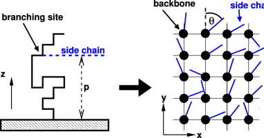
Figure 1: For describing as system of end-grafted, self-avoiding polymer backbones with rigid side chains (left), only the essential degrees of freedom, i.e. the height $p$ of the side chain above the substrate and its orientation angle $\theta$, are retained. A system of mutually interacting complexes is obtained by using a two-dimensional lattice of such rotors (right) where the dynamics is determined by Eq. (3).

We assume here that the sites at which the backbones are attached to the substrate are sufficiently far aparat from each other so that any interaction between the complexes is mediated by the side chains only. This also means that side chains only interact when they have the same height $p$. This aspect can be modeled by a Potts-type Hamiltonian Potts (1952); Wu (1982):

$$\mathcal{H}_{P}=-K_{P}\sum\limits_{\langle i,j\rangle}\delta_{p_{i}p_{j}}\,\,;\quad p_{i}\in\{0,1,\dots,q-1\}\,\,.$$ (1)

Here, $p_{i}$ denotes the height of side chain $i$ above the substrate, $q$ is the total number of allowed heights, and $K_{P}>0$ is the coupling constant (in units of $\beta=k_{B}T$).

The interaction between side chains with the same $p$ will be considered as a nearest-neighbor ferromagnetic interaction leading to a prefered parallel alignment of the side chains. This kind of interaction seems plausible as a first approach since it mimics the repulsive forces between side chains that may be due to steric or short-ranged electrostatic potentials. Consequently, we use for this part of the interaction the two-dimensional XY-model Hamiltonian:

$$\mathcal{H}_{XY}=-K_{XY}\sum\limits_{\langle i,j\rangle}\mathbf{S}_{i}\mathbf{S}_{j}=-K_{XY}\sum\limits_{\langle i,j\rangle}S_{i}S_{j}\cos\theta_{ij}\,\,,$$ (2)

with the coupling constant $K_{XY}>0$ and $\langle i,j\rangle$ denoting a summation over nearest neighbors. For simplicity, the length of the rotors (=side chains) $S_{i}=|\mathbf{S}_{i}|$ is set to unity while the angle $\theta_{ij}$ denotes the relative orientation of the side chains $i$ and $j$.

Combining the above models Eq. (1) and Eq. (2) yields the hybrid model that is used to describe the surface-attached polymer complexes of the extracellular matrix:

$$\mathcal{H}=-K\sum\limits_{\langle i,j\rangle}\delta_{p_{i}p_{j}}\,S_{i}S_{j}\cos\theta_{ij}\,\,;\quad p_{i}\in\{0,\dots,q-1\}\,\,.$$ (3)

The two-dimensional Potts model is known to undergo a second order phase transition for $q<4$ Baxter (1973) while the XY-model shows a Kosterlitz-Thouless transition Kosterlitz and Thouless (1974); Kosterlitz (1974). For $q=3$ our model Eq. (3) can be interpreted as a 3-state Potts model with a randomly varying coupling strength $K_{ij}=\cos\theta_{ij}$ between neighbouring Potts spins $i$ and $j$. As this local coupling may become very small and even zero, the nature of the phase transition of the hybrid model may be influenced by vacancies that are known to drive the transition of the ($q<4$)-state Potts model to a first order behavior Nienhuis et al. (1979). Given this variety of phase behaviors, it appears difficult to predict the system’s behavior a priori.

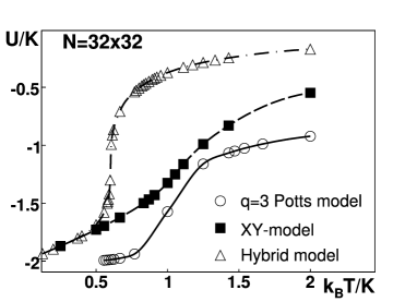
Figure 2: The inner energy $U$ per rotor shows a sigmoidal increase with temperature $T$ for the pure XY-model [Eq. (2)], the pure $3$-state Potts model [Eq. (1)], and the hybrid model [Eq. (3)]. The transition temperature $T_{c}$ for the latter appears to be shifted towards lower values while the slope in the transition region is strongly increased. Full lines are guides to the eye.

III Simulation Method

For simulations of the hybrid model Eq. (3) we relied on the Monte Carlo (MC) method (see, e.g., Binder and Heermann (2002) for an introduction). Far away from the critical temperature, we employed the Metropolis MC algorithm Metropolis et al. (1953). In each step, a rotation of each rotor (side chain) by some angle $\Delta\theta_{i}$ and a change of its Potts level (height) were proposed and this combined move was accepted or rejected for each rotor according to the Metropolis criterion.

Close to the critical temperature, the standard Metropolis MC suffers from critical slowing down, i.e. it becomes difficult to generate enough statistically independent configurations for a reliable statistics. To overcome this problem, we used a cluster MC approach Swendson and Wang (1987), i.e. a modification of Wolff’s cluster algorithm Wolff (1989). Here, one deals with two degrees of freedom, one discrete (Potts level $p$) and one continuous (orientation angle $\theta$). Thus, two different kinds of clusters are grown and flipped in each step – one with respect to $p$ (embedded in an ensemble of fixed $\theta_{i}$’s) and another one with respect to $\theta$ (embedded in an ensemble of fixed $p_{i}$’s).

The treatment of the Potts degree of freedom has to be carried out carefully as ferromagnetic and anti-ferromagnetic bonds can occur between neighboring rotors. In the beginning, a pair of values for $p$ is chosen randomly, i.e. (0,1), (0,2), or (1,2), respectively. Rotors in the remaining Potts state are kept unchanged, i.e.,the identity operator is applied, and thus do not contribute to the ongoing cluster growing step. The effective (local) coupling between rotors $i$ and $j$ is $K_{\rm eff}=K\cdot S_{i}S_{j}\cos\theta_{i,j}$. For $K_{\rm eff}>0$ a ferromagnetic bond is established with probability $P=1-\exp\left(-K_{\rm eff}\delta_{p_{i},p_{j}}\right)$ between rotors on the same Potts level. If $K_{\rm eff}<0$, an anti-ferromagnetic bond is formed with probability$P=1-\exp\left(K_{\rm eff}(1-\delta_{p_{i},p_{j}})\right)$ between rotors on different Potts levels. When the cluster is grown, all Potts levels of the involved rotors are switched according to the initially chosen pair of $p$-values (e.g. 0 $\leftrightarrow$ 1).

Following Wolff’s embedding trick for growing and flipping clusters in the XY-model Wolff (1989) the rotors are projected onto the $x$-axis. This results in an Ising model of the $x$-components $S^{x}_{i}$ with random couplings. These ’effective’ spins are connected by a bond with probability $P=1-\exp\left(\delta_{p_{i},p_{j}}\cdot\min[0,2KS^{x}_{i}S^{x}_{j}]\right).$ Please note that the Potts states of the rotors are accounted for by $\delta_{p_{i},p_{j}}$ meaning that bonds are only formed between rotors on the same Potts level. Finally, when the cluster is grown, all $x$-components of the constituing rotors are inverted.

IV Results

To study the thermodynamic properties of a system of interacting rotors modelled by the Hamiltonian Eq. (3) with $q=3$ we conducted extensive MC simulations using the method described in the preceeding section. The linear system size $L$ (i.e. using $N=L^{2}$ rotors) was varied in the range $32\leq L\leq 1024$ in order to apply a finite-size scaling analysis. We have concentrated here in particular on the inner (potential) energy $U$ per rotor and the transition temperature $T_{c}$.

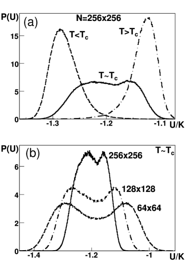
Figure 3: (a) The inner energy $U$ below and above the critical temperature $T_{c}$ shows only a single maximum for a system with $N=256$, while for $T\approx T_{c}$ a slight double-peak structure is observed. (b) Indeed, this double-peak structure at $T\approx T_{c}$ is even better visible for small systems and seems to subside for larger system sizes.

Metropolis MC simulations of small systems revealed significant differences in the behavior between the hybrid model and the two constituting models (Potts and XY). Fig. 2 shows the variation of $U$ with temperature for all three models. Obviously, the transition point $T_{c}$ of the hybrid model is much lower than those of the constituting models. Furthermore, the transition region is much steeper, suggesting a first-order transition. At this point, however, it cannot be determined if the slope really diverges at $T_{c}$ which would be a criterion for a discontinuous phase transition. This behavior would be qualitatively different from that shown by the constituting models, yet would agree with the random Potts model Nienhuis et al. (1979). Please note that for $T<T_{c}$ the energy $U$ of the hybrid model resembles essentially that of the corresponding pure XY-model. Thus, the Potts degree of freedom seems to be ’frozen’ in this regime while all excitations occur with respect to the XY-degree of freedom.

Figure 4: (a) The depth $\Delta=\ln[P(U)_{max}/P(U)_{min}]$ of the minimum between the double peak in $P(U)$ appears to vanish with system size $L$, thus indicating a second-order phase transition. (b) In agreement with this, the phase transition temperature shows a scaling $T_{c}\sim 1/L$. (c) The tendency of the 4^th-order cumulant towards a value $V=2/3$ is also in support of a second-order phase transition.

For a more thorough investigation, we used the cluster algorithm described in the preceeding section. In contrast to the standard Metropolis MC method it allowed for extensive simulations of large systems close to $T_{c}$ due to a reduced dynamic exponent. We focussed on the inner energy $U$ as we found no proper order parameter to follow the phase behavior of the hybrid model. As can be seen from Fig. 3a, the distribution $P(U)$ shows pronounced single peaks for $T\ll T_{c}$ and $T\gg T_{c}$, while for $T\approx T_{c}$ a double-peak seems to emerge. In Fig. 3b, the distribution $P(U)$ is shown for three different system sizes at $T\approx T_{c}$. The distributions were obtained by reweighting Ferrenberg and Swendson (1988) of distributions close to $T_{c}$. Our numerical data indeed highlight a double-peak structure in $P(U)$, indicating the coexistence of two phases and thus a first-order phase transition. To extrapolate if this finding persists in the thermodynamic limit, we first considered the logarithm of the relative gap depth $\Delta=\ln[P(U)_{max}/P(U)_{min}]$ at $T\approx T_{c}$ for growing system sizes $L$. For a first-order transition, this quantity is supposed to grow with $L$. In the hybrid model studied here, however, $\Delta\to 0$ for $L\to\infty$ (Fig. 4a). Thus, the energy distribution assumes a Gauss-like shape in the thermodynamic limit, consistent with a second-order phase transition with only a single phase existing in the system at $T_{c}$. Considering the finite-size scaling of the transition temperature $T_{c}$ with the inverse system size $1/L$ supports this notion since we find $T_{c}\propto 1/L$ as anticipated for a second-order transition (Fig. 4b).

Further evidence for a second order phase transition comes from the 4^th order cumulant of the energy distribution Binder (1981)

$$V=1-\frac{\langle U^{4}\rangle}{3\cdot\langle U^{2}\rangle^{2}}\,\,.$$ (4)

For a Gaussian distribution, this quantity takes on the value $V=\frac{2}{3}$ while distributions with a double-peak structure are characterized by $V\neq\frac{2}{3}$. While a small dip in $V(T)$ is observed for small system sizes (Fig. 4c), it subsides for large $L$ and only very small deviations from $V=2/3$ are seen. In the thermodynamic limit, one thus expects $V=\frac{2}{3}$, i.e. a Gauss(-like) distribution for all temperatures.

The phase behavior of the system above and below the critical temperature is shown in Fig. 5. While for $T<T_{c}$ the rotors (=rigid side chains) are ordered (Fig. 5a), they assume random orientations for $T>T_{c}$. The mean Potts level (=the average height of the rigid side chains) in both cases is $\langle q\rangle=1$ (Fig. 5c), yet for $T<T_{c}$ collective fluctuations of the rotors to the three degenerate Potts levels are observed. Given the small transition probabilities for these height fluctuations for fixed temperatures (which we circumvented via the MC cluster algorithm) the dwell time at an individual Potts levels may be very large.

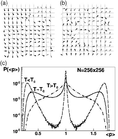
Figure 5: Snapshot of the system at (a) $T<T_{c}$ and (b) $T>T_{c}$. Rotor orientations are indicated by arrows, Potts levels $p=1,2,3$ are labeled in black, dark grey and light grey, respectively. (c) Probability distribution of the mean Potts level in the system $P(\langle p\rangle)$. In the ordered state at $T<T_{c}$ (dashed), all Potts states $p=1,2,3$ are populated with similar probabilities while for $T\approx T_{c}$ (dash-dotted) and $T>T_{c}$ (full) the state $p=1$ is clearly favored.

V Conclusions

In this work, we have proposed a model for a system of surface-attached polymers with rigid side chains that is found, e.g., in the extracellular matrix of mammalian cells. To reduce the computational effort when simulating large systems of end-grafted flexible polymers with rigid side chains, a coarse grained approach has been chosen combining two well-known models of statistical physics, namely the Potts and the XY-model. The thermodynamics of the ’hybrid’ model, given by the Hamiltonian Eq. (3), has been studied in Monte Carlo simulations and a second-order phase transition was found.

Given our results, it seems reasonable to call the hybrid model rather a ’modified Potts model’ than a ’modified XY-model’ as the phase behavior of the system is dominated by the 3-state Potts model: At low temperatures, the rotors essentially condensate into a single Potts state. This corresponds to the (three-fold degenerate) ground state of the Potts model showing long-range order with respect to $p$. Excitations in this regime arise due to perturbations in the ordered state of the XY-model. At high temperatures, the influence of the XY degree of freedom becomes manifest as a randomized coupling of the Potts spins which includes the existence of vacancies that may drive the transition of the 3-state Potts model from second to first order Nienhuis et al. (1979). Indeed, at first glance, the transition of the hybrid model appears to change character (cf. Fig. 2 and Fig. 3). Only more thorough investigations revealed the transition to be still continuous, i.e. to remain second order. Thus, the vacancies evoked by the random coupling drive the transition towards first order, but do not suffice to fully change its character.

Coming back to the original problem that inspired the model, i.e. the dynamics of the extracellular matrix, the observed ordering of the system for $T<T_{c}$ may actually be used by a cell to change the thickness of its protective layer. A cell may use the transition to the regime $T<T_{c}$ to freeze the extracellular matrix in a desired homogenous ordered state/height that is not necessarily ’thicker’ than in the disordered regime. Thus, speaking in terms of the original problem, the cell may tune the thickness of its extracellular matrix by tuning the interactions of the (polyelectrolytic) aggrecan side chains, thereby driving the system through the phase transition. It will be interesting to experimentally manipulate the aggrecan interaction by changing ion conditions for the extracellular matrix and thereby to induce the above described phase transition.