Molecular electronics in junctions with energy disorder

Abstract

We investigate transport through molecular wires whose energy levels are affected by environmental fluctuations. We assume that the relevant fluctuations are so slow that they, within a tight-binding description, can be described by disordered, Gaussian distributed onsite energies. For long wires, we find that the corresponding current distribution can be rather broad even for a small energy variance. Moreover, we analyse with a Floquet master equation the interplay of laser excitations and static disorder. Then the disorder leads to spatial asymmetries such that the laser diving can induce a ratchet current.

1 Introduction

Chemical adsorption of sulfur atoms on gold surface allows a stable bond between gold tips and thiol groups of molecules. This has been exploited for measuring the conductance and the current-voltage characteristics of gold-molecule-gold junctions [1, 2, 3, 4, 5, 6]. Repeated measurements even with the same sample, however, reveal small but noticeable differences which possibly stem from environmental fluctuations that impact upon the effective molecule parameters. Moreover, the particular form of the gold tip can have a significant influence on the transport properties [7].

A present line of experimental research is the measurement of molecular conductance when the electrons are excited by electromagnetic waves. There one expects various phenomena ranging from photo-assisted transport [8, 9] to ratchet or non-adiabatic pump effects, i.e. the induction of dc currents by ac fields even in the absence of any voltage bias [10, 11]. Moreover, it has been predicted that properly taylored laser pulses can give rise to short current pulses [12, 13, 14, 15]. Since a dc current flows into one particular direction, a ratchet effect can occur only in “sufficiently asymmetric” systems [9]. In that respect, a static disorder is sufficient to break the reflection symmetry of an individual realization and, thus, may support a ratchet effect.

The quantitative prediction of the current through a molecule is still a great challenge despite the significant progress achieved in recent years [16, 17, 18, 19]. For a more qualitative understanding of the mechanisms involved in molecular transport, it is thus advantageous to employ for the molecule a rather generic tight-binding model [20, 21, 22, 23, 8, 24, 9, 25]. Then a flexible method for the computation of transport properties is provided by master equations of the Bloch-Redfield type which allow one to include electron-electron and electron-phonon interactions, as well as time-dependent fields [9, 26]. Similar methods have also been used for describing incoherent transport [27, 28].

Here, we explore the role of slow fluctuations or static disorder for molecular conductance. Thereby we will assume that the relevant environmental fluctuations are so slow that they can be described as static disorder which defines an ensemble of wire Hamiltonians. Then a natural quantity of interest is the corresponding distribution of stationary currents. A setup for which this current distribution is also directly relevant is an array of molecular junctions that conduct in parallel. We employ a tight-binding model for the molecule and treat it with the Floquet master equation formalism derived in Ref. [26] which we review briefly in Section 2. In Section 3, we present results for a static model with a large voltage bias, while in Section 4, we investigate pumping effects caused by an interplay of ac driving fields and disorder. The analytical derivation of the current distribution for a wire with two sites is deferred to the Appendix.

2 Wire-lead model and master equation

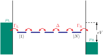
Figure 1: Bridged molecular wire model consisting of $N=5$ sites with internal tunnelling matrix elements $\Delta$ and effective wire-lead coupling strengths $\Gamma_{\mathrm{L/R}}$.

The system of the driven molecular wire, the leads, and the coupling between the molecule and the leads, as sketched in Fig. 1, is described by the Hamiltonian

$$\mathcal{H}(t)=\mathcal{H}_{\mathrm{wire}}(t)+\mathcal{H}_{\mathrm{leads}}+\mathcal{H}_{\mathrm{wire-leads}}.$$ (1)

The wire is modelled by $N$ tight-binding orbitals $|n\rangle$, $n=1,\ldots,N$, such that

$$\mathcal{H}_{\mathrm{wire}}=\sum_{n}(E_{n}(t)+\xi_{n})c_{n}^{\dagger}c_{n}-\Delta\sum_{n=1}^{N-1}(c_{n+1}^{\dagger}c_{n}+c_{n}^{\dagger}c_{n+1})+\frac{U}{2}\mathcal{N}(\mathcal{N}-1),$$ (2)

with the tunnel matrix element $\Delta$ and the capacitive energy $U$. Each onsite energy $E_{n}(t)+\xi_{n}$ contains a random contribution $\xi_{n}$ that subsumes the influence of environmental fluctuations. We assume that these fluctuations are Gaussian distributed and so slow that we can treat them as static disorder. Thus, the probability that the onsite energy of orbital $n$ lies in an interval of size $\mathrm{d}\xi$ around $E_{n}(t)+\xi_{n}$ reads

$$w(\xi_{n})=\frac{1}{\sqrt{2\pi\sigma^{2}}}\exp\Big{(}-\frac{\xi_{n}^{2}}{2\sigma^{2}}\Big{)},$$ (3)

where the variance $\sigma^{2}$ is assumed to be position-independent. This implies that the energy fluctuations are spatially uncorrelated, such that $\langle\xi_{n}\xi_{n^{\prime}}\rangle=\sigma^{2}\delta_{nn^{\prime}}$. The onsite energies $E_{n}(t)=E_{n}+Ax_{n}\cos(\Omega t)$ are modulated by a harmonically time-dependent dipole force, where $A$ denotes the electrical field amplitude multiplied by the electron charge and the distance between neighbouring sites, with $x_{n}=\frac{1}{2}(N+1-2n)$ the scaled position of site $|n\rangle$. Our goal will be to compute for many realizations of the wire Hamiltonian the resulting dc current which provides the current distribution $P(I)$. The last term in Eq. (2) captures the electron-electron interaction within a capacitor model and the operator $\mathcal{N}=\sum_{n}c_{n}^{\dagger}c_{n}$ describes the number of excess electrons residing on the molecule. Below we shall assume that $U$ is so large that only states with zero or one excess electron play a role. The first and the last site of the molecule, $|1\rangle$ and $|N\rangle$, couple via the tunnelling Hamiltonian

$$\mathcal{H}_{\mathrm{wire-leads}}=\sum_{q}(V_{\mathrm{L}q}\,c^{\dagger}_{\mathrm{L}q}c_{1}^{\vphantom{\dagger}}+V_{\mathrm{R}q}\,c^{\dagger}_{\mathrm{R}q}c_{N}^{\vphantom{\dagger}})+\mathrm{H.c.}$$ (4)

to the respective lead. The operator $c^{\dagger}_{\mathrm{L}q}$ ($c^{\dagger}_{\mathrm{R}q}$) creates an electron in the left (right) lead in state $|\mathrm{L}q\rangle$ which is orthogonal to all wire states. The influence of the tunnelling Hamiltonian is fully characterised by the spectral density $\Gamma_{\ell}(\epsilon)=2\pi\sum_{q}|V_{\ell q}|^{2}\delta(\epsilon-\epsilon_{q})$. If the lead states are dense and located at the centre of the conduction band, the spectral densities can be replaced by a constant, i.e. we assume $\Gamma_{\ell}(\epsilon)=\Gamma$ for both leads.

The leads are modelled as ideal Fermi gases

$$\mathcal{H}_{\mathrm{leads}}=\sum_{q}\big{(}\epsilon^{\vphantom{\dagger}}_{q\mathrm{L}}\,c^{\dagger}_{\mathrm{L}q}c^{\vphantom{\dagger}}_{\mathrm{L}q}+\epsilon^{\vphantom{\dagger}}_{q\mathrm{R}}\,c^{\dagger}_{\mathrm{R}q}c^{\vphantom{\dagger}}_{\mathrm{R}q}\big{)},$$ (5)

which are initially at thermal equilibrium with the chemical potential $\mu_{\mathrm{L}/\mathrm{R}}$ and, thus, are described by the density operator $\rho_{\mathrm{leads,eq}}\propto\exp{[-(\mathcal{H}_{\mathrm{leads}}-\mu_{\mathrm{L}}\mathcal{N}_{\mathrm{L}}-\mu_{\mathrm{R}}\mathcal{N}_{\mathrm{R}})/k_{\mathrm{B}}T]},$ where $\mathcal{N}_{\ell}=\sum_{q}c_{q\ell}^{\dagger}c_{q\ell}$ is the electron number operator for lead $\ell=\mathrm{L},\mathrm{R}$. Since a typical metal screens all electric fields with a frequency below the plasma frequency, we assume that the bulk properties of the leads are not affected by the laser irradiation.

2.1 Perturbation theory

The derivation of a master equation starts from the Liouville-von Neumann equation $\mathrm{i}\hbar\dot{\rho}(t)=[\mathcal{H}(t),\rho(t)]$ for the total density operator $\rho(t)$ for which one obtains by standard techniques the approximate equation of motion [29, 30, 31, 9, 32]

$$\dot{\rho}(t)=-\frac{\mathrm{i}}{\hbar}[H_{\mathrm{wire}}(t)+H_{\mathrm{leads}},\rho(t)]-\frac{1}{\hbar^{2}}\int_{0}^{\infty}\mathrm{d}\tau[H_{\mathrm{wire-leads}},[\widetilde{H}_{\mathrm{wire-leads}}(t-\tau,t),\rho(t)]].$$

Here the first term corresponds to the coherent dynamics of both the wire electrons and the lead electrons, while the second term describes resonant electron tunnelling between the leads and the wire. The tilde denotes operators in the interaction picture with respect to the molecule and the lead Hamiltonian without the molecule-lead coupling, $\widetilde{X}(t,t^{\prime})=U_{0}^{\dagger}(t,t^{\prime})\,X\,U_{0}(t,t^{\prime})$, where $U_{0}$ is the propagator without the coupling. The net (incoming minus outgoing) electrical current through the left contact is given by minus the time-derivative of the electron number in the left lead multiplied by the electron charge $-e$. From Eq. (2.1) follows for the current in the wide-band limit the expression

$$I_{\mathrm{L}}(t)=e\mathop{\mathrm{tr}}[\dot{\rho}(t)\mathcal{N}_{\mathrm{L}}]= -e\frac{\Gamma_{\mathrm{L}}}{\pi\hbar}\mathop{\mathrm{Re}}\int_{0}^{\infty}\mathrm{d}\tau\int\mathrm{d}\epsilon\,\rme^{\mathrm{i}\epsilon\tau/\hbar}$$ (6)

$$\times\big{\{}\langle c^{\dagger}_{1}\tilde{c}_{1}^{\vphantom{\dagger}}(t,t-\tau)\rangle\bar{f}_{\mathrm{L}}(\epsilon)-\langle\tilde{c}_{1}^{\vphantom{\dagger}}(t,t-\tau)c_{1}^{\dagger}\rangle f_{\mathrm{L}}(\epsilon)\big{\}},$$

where $f_{\ell}$ is the Fermi function of the respective lead and $\bar{f}_{\ell}=1-f_{\ell}$. Furthermore, $\langle\cdots\rangle=\mathop{\mathrm{tr}_{\mathrm{wire}}}\rho_{\mathrm{wire}}\cdots$ denotes the expectation value with respect to the wire density operator. We emphasise that the expectation values in Eq. (6) depend directly on the dynamics of the isolated wire and are thus influenced by the driving.

2.2 Floquet theory

An important feature of the current formula (6) is its dependence on solely the wire operators while all lead operators have been eliminated. Therefore it is sufficient to consider the reduced density operator $\rho_{\mathrm{wire}}=\mathop{\mathrm{tr}_{\mathrm{leads}}}\rho$ of the wire electrons. The effort necessary to calculate $\rho_{\mathrm{wire}}$ can be reduced significantly by exploiting the fact that the master equation (2.1) inherited from the total Hamiltonian $\mathcal{H}(t)$ a periodic time-dependence, which opens the way for a Floquet treatment.

One possibility for such a treatment is to use the Floquet states of the central system, i.e. the driven wire, as a basis. Thereby we also use the fact that in the wire Hamiltonian (2), the single-particle contribution commutes with the interaction term and, thus, these two Hamiltonians possess a complete set of common eigenstates. In analogy to the quasimomenta in Bloch theory for spatially periodic potentials, the quasienergies $\epsilon_{\alpha}$ come in classes $\epsilon_{\alpha,k}=\epsilon_{\alpha}+k\hbar\Omega,k\in\mathbb{Z},$ of which all members represent the same physical solution of the Schrödinger equation. Thus we can restrict ourselves to states within one Brillouin zone like for example $0\leq\epsilon_{\alpha}<\hbar\Omega$.

For the computation of the current it is convenient to have an explicit expression for the interaction picture representation of the wire operators. It can be obtained from the (fermionic) Floquet creation and annihilation operators defined via the transformation $c_{\alpha}(t)=\sum_{n}\langle\varphi_{\alpha}(t)|n\rangle c_{n},$ which reads in the interaction picture $\tilde{c}_{\alpha}(t,t^{\prime})=\mathrm{e}^{-\mathrm{i}(\epsilon_{\alpha}+U\mathcal{N}_{\mathrm{wire}})(t-t^{\prime})/\hbar}c_{\alpha}(t^{\prime}),$ with the important feature that the time difference $t-t^{\prime}$ enters only via the exponential prefactor [9].

2.3 Master equation and current formula

In the following, we assume the interaction $U$ to be the dominant energy scale in the system, therefore we can restrict the wire Hilbert space to the $N+1$ dimensional subspace of states with zero and one electron, such that a basis for the decomposition of the reduced operator is $\{|0\rangle,c_{\alpha}^{\dagger}(t)\,|0\rangle\}$, where $|0\rangle$ denotes the wire state in the absence of excess electrons. Moreover, it can be shown [26] that at large times, the density operator of the wire becomes diagonal in the electron number $\mathcal{N}$. Therefore a proper ansatz reads

$$\rho_{\mathrm{wire}}(t)=|0\rangle\rho_{00}(t)\langle 0|+\sum_{\alpha,\beta}c^{\dagger}_{\alpha}|0\rangle\rho_{\alpha\beta}(t)\langle 0|c_{\beta}.$$ (7)

Note that we keep terms with $\alpha\neq\beta$, which means that we work beyond a rotating-wave approximation.

Following our evaluation of the master equation [26], we arrive at a set of $N^{2}$ coupled equations of motion for $\rho_{\alpha\beta}(t)$ which in Fourier representation read

$$\mathrm{i}(\epsilon_{\alpha}-\epsilon_{\beta}-k\hbar\Omega)\rho_{\alpha\beta,k} = \frac{\Gamma_{\mathrm{L}}}{2}\sum_{k^{\prime},k^{\prime\prime}}\,\langle\varphi_{\alpha,k^{\prime}+k^{\prime\prime}}|1\rangle\langle 1|\varphi_{\beta,k+k^{\prime\prime}}\rangle\rho_{00,k^{\prime}}\big{(}f_{\mathrm{L}}(\epsilon_{\alpha,k^{\prime}+k^{\prime\prime}})+f_{\mathrm{L}}(\epsilon_{\beta,k+k^{\prime\prime}})\big{)}$$ (8)

$$-\frac{\Gamma_{\mathrm{L}}}{2}\sum_{\alpha^{\prime},k^{\prime},k^{\prime\prime}}\langle\varphi_{\alpha,k^{\prime}+k^{\prime\prime}}|1\rangle\langle 1|\varphi_{\alpha^{\prime},k+k^{\prime\prime}}\rangle\rho_{\alpha^{\prime}\beta,k^{\prime}}\,\bar{f}_{\mathrm{L}}(\epsilon_{\alpha^{\prime},k+k^{\prime\prime}})$$

$$-\frac{\Gamma_{\mathrm{L}}}{2}\sum_{\beta^{\prime},k^{\prime},k^{\prime\prime}}\langle\varphi_{\beta^{\prime},k^{\prime}+k^{\prime\prime}}|1\rangle\langle 1|\varphi_{\beta,k+k^{\prime\prime}}\rangle\rho_{\alpha\beta^{\prime},k^{\prime}}\,\bar{f}_{\mathrm{L}}(\epsilon_{\beta^{\prime},k^{\prime}+k^{\prime\prime}})$$

$$+\mathrm{same\ terms\ with\ the\ replacement}\>1,\mathrm{L}\rightarrow N,\mathrm{R}.$$

In an analogous manner we obtain for the dc current the expression

$$I_{\mathrm{L}} = \frac{e\Gamma_{\mathrm{L}}}{\hbar}\mathop{\mathrm{Re}}\sum_{\alpha,k}\Big{(}\sum_{\beta,k^{\prime}}\langle\varphi_{\beta,k^{\prime}+k}|1\rangle\langle 1|\varphi_{\alpha,k}\rangle\rho_{\alpha\beta,k^{\prime}}\bar{f}_{\mathrm{L}}(\epsilon_{\alpha,k})$$ (9)

$$-\sum_{k^{\prime}}\langle\varphi_{\alpha,k^{\prime}+k}|1\rangle\langle 1|\varphi_{\alpha,k}\rangle\rho_{00,k^{\prime}}f_{\mathrm{L}}(\epsilon_{\alpha,k})\Big{)}.$$

The results of this section allow us to numerically compute the dc current through a driven conductor as well as studying the undriven limit. The current distributions discussed below are obtained by computing the dc current for typically $10^{4}$ realizations of the wire Hamiltonian (2). Then these values are taken for a histogram with 150 bins which finally will be scaled such that we obtain a normalised probability density.

3 Electron transport with slowly fluctuating energies

We first address an undriven wire in the configuration sketched in Fig. 1 where the distribution of all wire levels is centred at energy $E_{n}=0$. The transport voltage is so large that all eigenenergies lie well within the voltage window and, consequently, the transport is unidirectional. Then in the absence of onsite energy fluctuations ($\sigma=0$), the current can be evaluated analytically within a rotating-wave approximation and reads $I_{\mathrm{max}}=e\Gamma/\hbar(N+1)$, i.e. it decays with increasing wire length [33]. The index “max” refers to the fact that any modification of the onsite energies can only reduce the current—which is confirmed by our simulations. The physical reason for this is that for equal onsite energies, solely the kinetic energy determines the eigenstates which, consequently, are delocalised. Different onsite energies, by contrast, tend to “localise” the eigenstates. Thus in the limit of small disorder, the current distribution $P(I)$ is expect to possess a clear peak at $I=I_{\mathrm{max}}$ and some minor contribution for lower values of $I$.

Figure 2 shows the simulated current distributions for two different variances. For a small variance (panel a), the distributions for short wires show the expected behaviour. With an increasing wire length, the peak at $I=I_{\mathrm{max}}$ disappears and is eventually replaced by an apparently parabolic distribution. This length dependence can be understood in the following way: For a short wire, the probability that a level is out of resonance is rather low and, thus, most realizations of the wire Hamiltonian will allow resonant inter-site tunnelling. With an increasing number of levels, however, the probability for having at least one misaligned level increases and a current significantly smaller than $I_{\mathrm{max}}$ becomes more likely. The precise values will depend on the details and, consequently, we expect a broad distribution. This means that whenever a large number of levels plays a role, the transport through a molecule is extremely sensitive to even small disorder induced by environmental fluctuations.

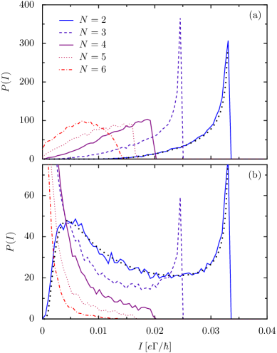
Figure 2: Current distribution for a channel with $N$ sites in the limit of a large bias voltage. The standard deviation of the onsite energies is $\sigma=0.5\Delta$ (a) and $\sigma=2\Delta$ (b), while the wire-lead coupling is $\Gamma=0.1\Delta$. The distributions have been obtained by computing the current for $1.5\times 10^{4}$ realizations of the wire Hamiltonian. The black dotted lines mark the analytical results for $N=2$ sites.

With a larger variance, this scenario becomes even more pronounced as can be seen in Fig. 2b: Then the peak at $I_{\mathrm{max}}$ is rather small and noticeable only for 2 and 3 sites. The most likely realization is a completely disordered wire with an accordingly low conductance. For $N>3$, the distributions even possesse a significant peak at $I=0$ which corresponds to isolating behaviour. A closer inspection of the numerical data reveals that the crossover between conducting and isolating behaviour occurs when the effective disorder $\sqrt{N}\sigma$ exceeds the tunnel matrix element $\Delta$.

Interestingly enough, for $N=2,3$ the distribution turns out to be even non-monotonic, which means that most one most likely finds either a current close to the theoretical maximum or a significantly smaller lower value. The non-monotonic behaviour for $N=2$ can also be found analytically. The derivation of the corresponding current distribution (12) can be found in the Appendix. The excellent agreement of this analytical solution and the simulated distributions emphasis that the simulation with approximately $10^{4}$ realisations ensures good convergence.

4 AC-driven disordered junctions

In order to investigate the influence of an AC driving, we employ the same model as above, but now with an additional dipole driving modelled by time-dependent onsite energies $E_{n}(t)=Ax_{n}\cos(\Omega t)$ as discussed in Sect. 2. The driving frequency $\Omega=2\Delta/\hbar$ is chosen such that it matches the average splitting of the wire energies, while the amplitude $A=\Delta$ corresponds to intermediately strong driving. The solid line in Fig. 3 shows the current distribution in the absence of a voltage bias, $V=0$. The reflection symmetry of the ensemble relates to the symmetric shape of the distribution, which implies that the current vanishes in the ensemble average. An individual realization of the wire, however, generally does not possess reflection symmetry because the random energy shifts are spatially uncorrelated. This asymmetry in combination with the non-adiabatic driving induces a coherent ratchet current, i.e. a dc current even in the absence of any net voltage bias. In the present case, the ratchet current is of the order of 10–20 percent of the current observed above in the large bias limit. This order of magnitude is typical when the driving frequency or a multiple of the driving frequency lies close to an internal resonance, while the intensity is moderate [26]. In addition to the broad distribution of ratchet currents, $P(I)$ exhibits a peak at $I=0$. This stems from realizations for which the driving is well out of resonance.

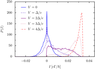
Figure 3: Current distribution for an AC driven wire with $N=2$ sites for various bias voltages. The fluctuations of the onsite energies are characterised by the standard deviation $\sigma=0.5\Delta$, the driving frequency and amplitude are $A=\Delta$ and $\Omega=2\Delta/\hbar$, respectively. All the other parameters are as in Fig. 2.

For a bias voltage $V>0$, the ensemble no longer possesses reflection symmetry and the current distribution is shifted towards positive values (see Fig. 3). For sufficiently small voltages $V\lesssim\Delta/e$, non-adiabatic pumping against the voltage bias is still possible. Rather surprisingly, the peak at zero current remains. It now corresponds to realizations for which on the one hand, the driving is off-resonant while on the other hand, both levels lie outside the voltage window. With an increasing bias voltage, the second condition is less frequently fulfilled, and eventually the distribution assumes a form similar to that found for a large voltage in the absence of driving. Already for $V\approx 4\Delta/e$, the distribution is hardly distinguishable from the one shown in Fig. 2a for a wire with $N=2$ sites in the absence of driving.

5 Conclusions

We have investigated the current through a molecular wire with disordered onsite energies. Such a disorder can stem from the interaction with slow fluctuations of background charges in the substrate. In particular, we computed the resulting current distribution for two typical cases, namely an “open transport channel” and a driven molecular wire for which random energy shifts break reflection symmetry and, thus, the driving can induce a ratchet current.

The open transport channel is characterised by tight-binding levels with equal onsite energies, such that any misalignment stems from the disorder. Its main consequence is that as soon as the standard deviation of the onsite energies exceeds the tunnel matrix elements, the current distribution no longer peaks only at a finite value, but also at zero. For longer wires, only the peak at zero current remains. This isolating behaviour resembles Anderson localisation which is found for electrons in a one-dimensional disordered lattice [34]. Note however, that we here considered short wires far from the scaling limit in which Anderson localisation is usually studied.

Since the random energy shifts break reflection symmetry, driving the molecular wire with a laser field induces ratchet currents for which we found a relatively broad distribution. If the driving frequency is far from any molecular excitation energy, the ratchet current will be rather small, and we indeed found that this is the case for very many wire realizations. It has the consequence that the corresponding distribution possesses a spike at zero current. This means that non-adiabatic pumping of electrons against a voltage bias becomes generally impossible whenever the relevant wire energy levels lie well within the voltage window.

In conclusion, our results reveal that slow fluctuations or a static disorder can have a significant effect on molecular conduction. In various cases, the current distribution emerges to be rather flat, which means that even the magnitude of the current depends sensitively on environmental influences.

Appendix A Analytical solution for two levels

A wire model with $N=2$ sites represents an analytically solvable case for which one observes a non-monotonic current distribution and which can serve as test case for numerical implementations. Here we consider a two-level system with on-site energies $\xi_{1,2}$, i.e. with a bias $2\eta=\xi_{1}-\xi_{2}$. Since the random energy shifts $\xi_{n}$ are Gaussian distributed with variance $\sigma^{2}$, the bias $2\eta$ is also Gaussian distributed but with variance $2\sigma^{2}$, i.e. its distribution function reads $w(\eta)=\exp(-\eta^{2}/\sigma^{2})/\sqrt{\pi\sigma^{2}}$.

For the computation of the current, we restrict ourselves to the limit of a large transport voltage such that both eigenenergies of the two-level system lie within the voltage window. Then, the Fermi functions of the left and the right lead effectively become $f_{\mathrm{L}}=1$ and $f_{\mathrm{R}}=0$. In this case, transport can be described within rotating-wave approximation (RWA) which practically means that the reduced density operator of the wire is diagonal in energy representation [33]. Within RWA thus follows from the master equation (8) the occupation probability $\rho_{\alpha\alpha}=w_{\alpha}^{1}/w_{\alpha}^{2}$ and, thus, $\rho_{00}=1-\sum_{\alpha}w_{\alpha}^{1}/w_{\alpha}^{2}$. The coefficients $w_{\alpha}^{n}=|\langle\phi_{\alpha}|n\rangle|^{2}$ denote the overlap between the eigenstate $|\phi_{\alpha}\rangle$ and the localised state $|n\rangle$ (Note that in the undriven case, all non-vanishing contributions have sideband index $k=0$, such that here the sideband index $k$ can be omitted). Inserting this solution into the current formula (9), we obtain $I=e\Gamma/\hbar(1+\sum_{\alpha}w_{\alpha}^{1}/w_{\alpha}^{2})$.

The remaining task is now to diagonalise the single-particle Hamiltonian which provides the coefficients $w_{\alpha}^{n}$. For bias $2\eta$ and tunnelling matrix element $\Delta$, the Hamiltonian in pseudo-spin notation reads $H=\eta\sigma_{z}+\Delta\sigma_{x}$ and possesses the eigenenergies $\pm\delta=\pm(\eta^{2}+\Delta^{2})^{1/2}$. The corresponding eigenvectors $\phi_{\alpha}$ are proportional to $(\delta+\eta,\Delta)$ and $(\delta-\eta,\Delta)$, respectively, such that $w_{\alpha}^{1}/w_{\alpha}^{2}=(\delta\pm\eta)^{2}/\Delta^{2}$. Then we obtain for the current the expression

$$I(\eta)=\frac{e\Gamma}{\hbar}\frac{1}{3+4\eta^{2}/\Delta^{2}}=\frac{I_{\mathrm{max}}}{1+4\eta^{2}/3\Delta^{2}},$$ (10)

which assumes its maximum $I_{\mathrm{max}}=e\Gamma/3\hbar$ in the unbiased limit $\eta=0$.

The probability distribution for the current relates to $w(\eta)$ via

$$P(I)=\sum_{i}w(\eta_{i})\Big{|}\frac{\mathrm{d}\eta_{i}}{\mathrm{d}I}\Big{|},$$ (11)

where the summation considers all values of $\eta$ that fulfil the condition $I=I(\eta)$. After some straightforward algebra, we obtain by evaluating expression (11) the current distribution

$$P(I)=\sqrt{\frac{3\Delta^{2}}{4\pi\sigma^{2}}}\frac{I_{\mathrm{max}}/I^{2}}{\sqrt{I_{\mathrm{max}}/I-1}}\exp\Big{(}-\frac{3\Delta^{2}}{4\sigma^{2}}(I_{\mathrm{max}}/I-1)\Big{)},$$ (12)

which is defined and normalised on the interval $[0,I_{\mathrm{max}}]$.

References

References

- [1] Datta S, Tian W, Hong S, Reifenberger R, Henderson J I and Kubiak C P 1997 Phys. Rev. Lett. 79 2530
- [2] Reed M A, Zhou C, Muller C J, Burgin T P and Tour J M 1997 Science 278 252
- [3] Kergueris C, Bourgoin J P, Palacin S, Esteve D, Urbina C, Magoga M and Joachim C 1999 Phys. Rev. B 59 12505
- [4] Cui X D, Primak A, Zarate X, Tomfohr J, Sankey O F, Moore A L, Moore T A, Gust D, Harris G and Lindsay S M 2001 Science 294 571
- [5] Reichert J, Ochs R, Beckmann D, Weber H B, Mayor M and von Löhneysen H 2002 Phys. Rev. Lett. 88 176804
- [6] Dadosh T, Gordin Y, Krahne R, Khivrich I, Mahalu D, Frydman V, Sperling J, Yacoby A and Bar-Joseph I 2005 Nature 436 677
- [7] Yaliraki S N and Ratner M A 1998 J. Chem. Phys. 109 5036
- [8] Platero G and Aguado R 2004 Phys. Rep. 395 1
- [9] Kohler S, Lehmann J and Hänggi P 2005 Phys. Rep. 406 379
- [10] Lehmann J, Kohler S, Hänggi P and Nitzan A 2002 Phys. Rev. Lett. 88 228305
- [11] Strass M, Hänggi P and Kohler S 2005 Phys. Rev. Lett. 95 130601
- [12] Franco I, Shapiro M and Brumer P 2007 Phys. Rev. Lett. 99 126802
- [13] Li G Q, Schreiber M and Kleinekathöfer U 2007 EPL 79 27006
- [14] Kohler S and Hänggi P 2007 Nat. Nanotechnol. 2 675
- [15] Fainberg B D, Jouravlev M and Nitzan A 2007 Phys. Rev. B 76 245329
- [16] Di Ventra M, Pantelides S T and Lang N D 2000 Phys. Rev. Lett. 84 979
- [17] Damle P, Ghosh A W and Datta S 2002 Chem. Phys. 281 171
- [18] Heurich J, Cuevas J C, Wenzel W and Schön G 2002 Phys. Rev. Lett. 88 256803
- [19] Evers F, Weigend F and Koentopp M 2004 Phys. Rev. B 69 235411
- [20] Mujica V, Kemp M and Ratner M A 1994 J. Chem. Phys. 101 6849
- [21] Segal D, Nitzan A, Davis W B, Wasielewski M R and Ratner M A 2000 J. Phys. Chem. 104 3817
- [22] Foa Torres L E F, Pastawski H M and Makler S S 2001 Phys. Rev. B 64 193304
- [23] Čížek M, Thoss M and Domcke W 2004 Phys. Rev. B 70 125406
- [24] del Valle M, Tejedor C and Cuniberti G 2005 Phys. Rev. B 71 125306
- [25] del Valle M, Gutirrez R, Tejedor C and Cuniberti G 2007 Nat. Nanotechnol. 2 176
- [26] Kaiser F J, Hänggi P and Kohler S 2006 Eur. Phys. J. B 54 201
- [27] Petrov E G and Hänggi P 2001 Phys. Rev. Lett. 86 2862
- [28] Lehmann J, Ingold G L and Hänggi P 2002 Chem. Phys. 281 199
- [29] Bruder C and Schoeller H 1994 Phys. Rev. Lett. 72 1076
- [30] Gurvitz S A and Ya. S. Prager 1996 Phys. Rev. B 53 15932
- [31] Lehmann J, Kohler S, May V and Hänggi P 2004 J. Chem. Phys. 121 2278
- [32] Brandes T 2005 Phys. Rep. 408 315
- [33] Kaiser F J, Strass M, Kohler S and Hänggi P 2006 Chem. Phys. 322 193
- [34] Anderson P W 1958 Phys. Rev. 109 1492