Realistic modelling of quantum point contacts subject to high magnetic fields and with current bias at out of linear response regime

Abstract

The electron and current density distributions in the close proximity of quantum point contacts (QPCs) are investigated. A three dimensional Poisson equation is solved self-consistently to obtain the electron density and potential profile in the absence of an external magnetic field for gate and etching defined devices. We observe the surface charges and their apparent effect on the confinement potential, when considering the (deeply) etched QPCs. In the presence of an external magnetic field, we investigate the formation of the incompressible strips and their influence on the current distribution both in the linear response and out of linear response regime. A spatial asymmetry of the current carrying incompressible strips, induced by the large source drain voltages, is reported for such devices in the non-linear regime.

I Introduction

The new era of quantum information processing attracts an increasing interest to investigate the intrinsic properties of small-scale electronic devices. One of the most interesting of such devices is the so called quantum point contacts (QPCs), where a quantized current is transmitted through it under certain conditions van Wees et al. (1988); Wharam et al. (1988). They are constructed on two dimensional electron systems (2DES) either by inducing electrostatic potential on the plane of 2DES and/or by chemically etching the structure. The essential physics is that, the small size of the constraint creates quantized energy levels in one dimension (perpendicular to the current direction) therefore, transport takes place depending on whether the energy of the electron coincides with this quantized energy or not. In the ideal case at low bias voltages, if the energy of the electron is smaller then the lowest eigen-energy of the constraint, no current can pass through the QPC. Otherwise, only a certain integer number of levels (channels) are involved, therefore conductance is quantized Davies (1998). Beyond being a useful play ground for the basic quantum mechanical applications many other interesting features are reported in the literature such as the 0.7 conductance anomaly Thomas et al. (1996a); Kristensen et al. (1998); Thomas et al. (1996b), which became a paradigm since then. Another adjustable parameter which induces quantization on the 2DES is the magnetic field $B$ applied perpendicularly to the system. Such an external field changes not only the density of states (DOS) profile of the 2DES but also the screening properties of the system drastically. The interesting physics dictated by this quantization is observed as the quantum Hall effects v. Klitzing et al. (1980); Tsui et al. (1982). Recent theoretical investigations point out the importance of the electron-electron interactions in explaining the integer quantum Hall effect Siddiki and Gerhardts (2004a); Siddiki (2008a), believed to be irrelevant in the early days of this field Kramer et al. (2003), which we discuss briefly in this work. The basic idea behind the inclusion of the interaction is as follows: due to the perpendicular magnetic field the energy spectrum is discrete, known as the Landau levels (LLs), and is given by $E_{n}=\hbar\omega_{c}(n+1/2)$ where $n$ is a positive integer and cyclotron energy is defined as $\hbar\omega_{c}=\hbar eB/m^{*}$, with effective electron mass $m^{*}=0.067*m_{e}$. Taking into account the finite size of the sample, i.e. the confinement potential, and the mutual interaction (Hartree) potential, one obtains the total potential. In the next step for a fixed average electron density one calculates the resulting electron density distribution and from this distribution re-calculates the potential distribution iteratively. This self-consistent calculation ends in formation of the compressible and incompressible regions. In a situation where Fermi energy $E_{F}$ is pinned to one of the LLs, then the system is compressible. Otherwise, if $E_{F}$ falls in between two consecutive LLs, the system is known to be incompressible and, since there are no available states at the $E_{F}$ for electrons to be redistributed, screening is poor. However, within these incompressible regions the resistivity vanishes, hence all the applied current is confined to these regions. We will be discussing the details of this model in Sec.IV.

Most recently, the experiments performed at the 2DES including the QPCs, in the presence of an external magnetic field, manifested peculiar results Ji et al. (2003); Aidala et al. (2007); Roddaro et al. (2005). In the first set of experiments electron interference, such as Mach-Zehnder (MZ) Ji et al. (2003); Neder et al. (2006); Litvin et al. (2007); Roulleau et al. (2007a); Litvin et al. (2008); Roulleau et al. (2007b) and Aharonov-Bohm (AB) Camino et al. (2005), was investigated. The MZ interference experiments exhibit a novel and yet unexplained behavior, regarding the interference contrast (visibility) at the interferometer in the nonlinear transport regime (finite transport voltage). As a function of voltage, the visibility displayed oscillations whose period was found to be independent of the path lengths of the interferometer, in striking contrast to any straightforward theoretical model (e.g. using Landauer-Büttiker edge states (LBES) Büttiker (1986)). In particular, a new energy scale, of order of $\mu$eV, emerged, determining the periodicity of the pattern. This unexpected behavior of interfering electrons is believed to be related to electron-electron interactions Ji et al. (2003). The most satisfying model existing in the literature is proposed by I. P. Levkivskyi and E. V. Sukhorukov Levkivskyi and Sukhorukov (2008). However, other schemes also including interactions are present Chalker et al. (2007) and models, which consider a non-Gaussian noise as a source of the visibility oscillations Neder and Marquardt (2007), without interaction. The novel magnetic focusing experiments concerning QPCs has revealed the scattering processes taking place near these devicesAidala et al. (2007). It was explicitly shown that, the experimental realization of the sample and the device itself strongly effects the transport properties. It is reported that, the potential profile generated by the donors (impurities) and the gates deviates strongly from the ideal ”point” contact. Even in each cool down process, since the impurity distribution changes, the quantum interference fringes differ considerably. Hence a realistic modelling of a QPC is desirable, which we partially attack in this work. Another interesting set of experiments within the integer quantum Hall regime is conducted by S. Roddaro et.alRoddaro et al. (2005), where the transmission is investigated as a function of the gate bias. The findings show that current transmission strongly deviates from the expected chiral Luttinger liquid Sarma and Pinczuk (1997) behavior, since the transmission is either enhanced or suppressed by changing the gate bias. This effect was attributed to the particle hole symmetry of the Luttinger liquid and is discussed in detail in Ref.[Lal, 2007]. However, the explicit treatment of the QPC was left unresolved. Since the essential physics can be still governed by considering a finite size QPC opening, therefore assuming formation of a (integer) filling region sufficient.

The theoretical investigation of QPCs covers a wide variety of approaches, which can be grouped into two: i) the models that include electron-electron interactions and ii) the models that do not. At the very simple model in describing the QPCs, one considers a potential barrier perpendicular to the current direction quantizing the energy levels. Therefore the electrons are considered to be plane waves before they reach to the QPC and transmission and reflection coefficients are calculated from this potential profile. A better (2D) approximation is to model the QPCs with well defined functionsChklovskii et al. (1993); Meir et al. (2002), such as ellipses which lead to analytic solutions for the energy eigenfunctions and energies. About a decade ago J. Davies and his co-workers developed the ”frozen charge” model Davies and Larkin (1994) to calculate the potential profile induced by the gates defining the QPC. This approach is still one of the most used technique to obtain the potential profile, however, it is not self-consistent and completely ignores the donors and surface charges. There exists many theories which takes the potential profile from the frozen charge model as an initial condition, and provides explicit calculation schemes to obtain charge, current and potential distributions Ihnatsenka and Zozoulenko (2006); Rejec and Meir (2006); Siddiki and Marquardt (2007); Siddiki et al. (2008a); Siddiki (2008b). One of the most complete scheme, even in the presence of an external $B$ field, is the local spin density approximation (LSDA) within the density functional theory (DFT) Kohn and Sham (1965). The LSDA+DFT Ihnatsenka and Zozoulenko (2007a, b); Rejec and Meir (2006) approaches are powerful to describe the essential physics of density distribution and even 0.7 anomaly phenomenologically, however, the description of the current distribution is still under debate. The scattering problem through the QPCs is usually handled by the ”wave packet” formalism and is very successful in explaining the magnetic focusing experiments. However, the potential profile is not calculated self-consistently and therefore, the effect of the incompressible strips resulting from electron-electron interaction is not taken in to account.

Back to early days of the theories that account for electron interactions, i.e. Chklovskii, Shklovskii and Glazman Chklovskii et al. (1992) (CSG) and Chklovskii, Matveev and Shklovskii Chklovskii et al. (1993) (CMS) models, the influence of the formation of the incompressible strips has been highlighted. In the CMS paper, it was even conjectured that, ’the ballistic conductance of the QPC in strong magnetic field is given by the filling factor at the saddle point of the electron density distribution multiplied by $e^{2}/2\pi\hbar$’, which is quantized only if an incompressible strip (region) resides at the saddle point. In one of the recent approaches, in the presence of a strong $B$ field, the electron-electron interaction is treated explicitly within the Thomas-Fermi approximation (TFA) self-consistently, meanwhile the current distribution is left unresolved Siddiki and Marquardt (2007). In this model, similar to other approaches, the bare confinement potential is obtained from the ”frozen charge” approximation, which in turn lead to discrepancies due to its non-self-consistent approach. Here, we improve on this previous work in two main aspects: i) the electrostatic potential is obtained self-consistently in 3D, which allows us to treat also the etched structures ii) the current distribution is calculated explicitly using the local version of the Ohm’s law, also in the out of linear response regime. We organize our work as follows: In Sec.II, we briefly describe the numerical scheme to calculate the potential profile at $B=0$ following Ref.[Weichselbaum and Ulloa, 2003], which is based on iterative solution of the Poisson equation in 3D. In particular, we study the effect of different gate geometries and focus on the comparison of the potential profiles of gate and etch defined QPCs. The numerical scheme to calculate potential and density profiles at finite temperature and magnetic field is introduced in Sec.III. Here, we review the essential ingredients of the TFA and discuss the limitations of our approach. Sec.IV is dedicated in investigating the current distribution within the local Ohm’s law Güven and Gerhardts (2003); Siddiki and Gerhardts (2004a); Siddiki (2007), where we consider both the linear response (LR) and out of linear response (OLR) regimes. In the OLR, we show that the large current bias induces an asymmetric distribution of the incompressible strips, due to the tilting of the Landau levels resulting from the position dependent chemical potential. We conclude our work by a summary.

II Electrostatics in 3D

The realistic modelling of 2DES relies on solving the 3D Poisson equation for given boundary conditions, set by the hetero-structure (GaAs/AlGaAs in our calculations) and the gate pattern, which describes the charge and potential distribution. The hetero-structure, shown in Fig.1a, consists of (metallic) surface gates (dark semi-elliptic regions on surface), a thin donor layer (denoted by light thin layer and $\delta$ Silicon doping) which provides electrons to the 2DES and the 2DES itself indicated by minus signs confined to a thin area. The 2DES is formed at the interface of the hetero-structure. The average electron density $\overline{n_{\rm el}}$ (and its spatial distribution $n_{\rm el}(x,y)$) is dictated by the donor density $\overline{n_{0}}$ and the metallic gates. Once the number of donors and the gate voltage $V_{G}$ are fixed, the potential and charge distribution of the system can be obtained by solving the Poisson equation, self-consistently.

For typical nanoscale devices with many (or at least a few) electrons in each of the electrostatically-defined regions, the charge distribution and the major energy scales are described to a good approximation by classical electrostatics. Due to the strong electric fields generated by segregating charge in a 2DES, the Coulomb energy is the dominant energy scale. In this sense, it is desirable to have a self-consistent electrostatic description of the system if one expects a good quantitative description thereof.

For solving the electrostatics of the system in three dimensions we used a code developed and successfully applied in previous studies Weichselbaum and Ulloa (2006); Weichselbaum and Ulloa (2003). It is based on a 4^th order algorithm operating on a square grid. The code allows flexible implementation of many boundary conditions relevant for nanoscale electrostatics: standard boundaries such as conducting regions at constant voltage (potential gates), of constant charge (large quantum dots) or charge density (doping), but also boundaries such as a depletable 2DEG, dielectric boundaries and surfaces of semiconductors with the Fermi energy pinned due to surface charges. Since the calculation is constrained to a finite volume of space including the surface of the sample, the outer boundary is considered open and is also obtained self-consistently along with the rest of the calculation.

Overall the code provides a reliable description of the potential landscape and thus the electric field as well as the charge distribution for the sample under consideration.

As an illustrating example in Fig.1 we show the hetero-structure under investigation together with the charge distributions at different layers. Area of the unit cell is $1.5\times 1.5$ $\mu$m², whereas the hight is chosen to be $156$ nm. The donor and the electron layer lies $43$ nm and $56$ nm below the surface, respectively. The metallic gates are deposited on the surface of the structure and are biased with $-1.7$ V and a homogeneous donor distribution is assumed, Fig. 1c. The induced charge distribution on the metallic gates exhibits apparent inhomogeneities shown in Fig.1b. The electrons are accumulated near the boundaries of the gates, a well known behavior for metallic boundary conditions. However, here we provide the explicit distribution which strongly differs from the previously used ”frozen charge” model where only a constant potential profile is assumed. The influence of these induced charges become more important when considering an external $B$ field. Since, the steepness of the external potential profile determines the effective widths of the current carrying incompressible strips. We should note that, our self-consistent model enables us also to handle the (side) surface charges which becomes important when considering chemical etching. In the following part we investigate systematically, the effects of the gate voltage and the device geometry on the electrostatic quantities.

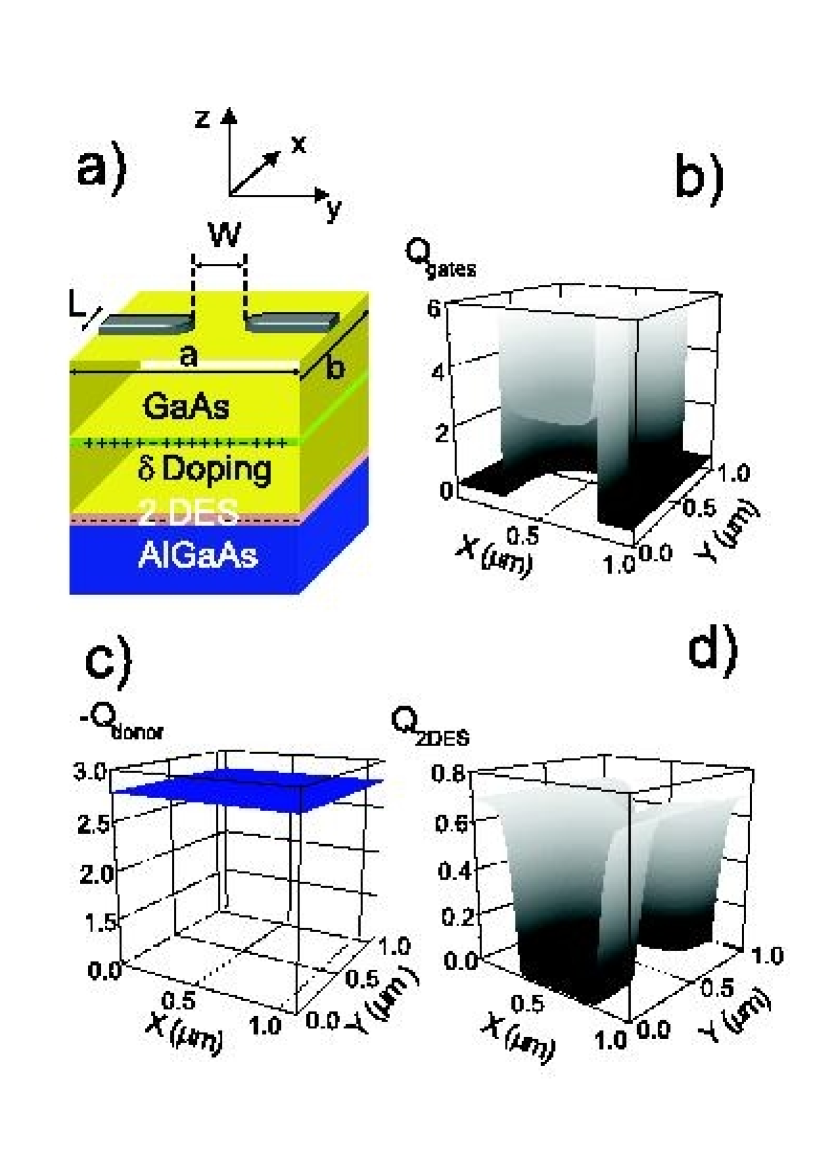
Figure 1: (Color online) (a) The Silicon doped hetero-structure, the 2DES is formed at the interface of the GaAs/AlGaAs (denoted by minus signs) and the metallic gates are deposited on the surface. At zero gate bias, the electron density is determined by the number of donors, which we chose to be $4\times 10^{16}$ cm^-2. Charge distribution at different layers, at the gates (b), the dopant layer (c) and the 2DES (d). It is clearly seen that not all the excess electrons are captured by the 2DES, rather a significant amount is accumulated on the surface. The electrostatic quantities are normalized with the relevant scales, i.e. charge (density) is normalized with the average electron density (e.g. ${\rm Q}_{\rm 2DES}(x,y)=n_{\rm el}(x,y)/\bar{n}_{\rm el}$) and electrostatic potential (energy) with the potential energy of a single electron.

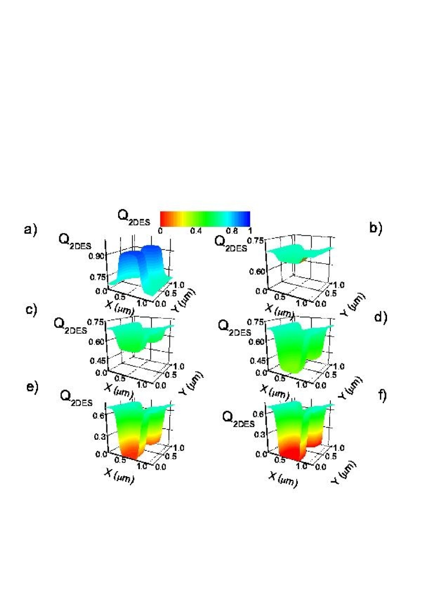
Figure 2: (Color online) Spatial distribution of the electrons as a function of the gate voltage. At zero bias (a) more electrons are populated under the gate which changes till depletion starts (b-d), where the gate voltage is set to be (b) -0.3V (c) -0.7V (d) -1.0 V. Almost no electrons are left beyond -1.5V applied to the gates, (e) -1.5V (f) -2.0 V.

II.1 Gate defined QPCs

In this subsection we compare the electron density profiles calculated for different QPC geometries applying various bias voltages, which exhibits strong non-linear behavior in contrast to many models used in the literature. We start our discussion with a rather smooth configuration, where the distance between the gates ($W$) is chosen to be $200$ nm (see Fig.1a). In Fig. 2 we show the cross section of the electron density profile for different gate voltages. Interestingly, at $V_{G}=0$ we see that more electrons are residing beneath the gates. This effect is due to inhomogeneous (induced) charge distribution at the metallic gates similar to the distribution shown in Fig.1d. The induced charges are mostly accumulated near the gate boundaries, whereas the center of the gates has almost a constant charge profile. Increasing $V_{G}$ to -0.3 Volts, already starts to depopulate electrons under the gates and the depopulation rate remains linear to the applied gate potential until the 2DES becomes depleted. In the $[-0.5,-1.2]$ Volt interval, the density distribution changes relatively smooth, since the electrons can still screen the external potential quite well. It is important to recall that, in the absence of an external $B$ field, the DOS of a 2DES is just a constant $D_{0}$ ($=m^{*}/\pi\hbar^{2}=2.83\times 10^{10}$ meV^-1 cm^-2 for GaAs), which is set by the sample properties, therefore screening is nearly perfect. Whereas this changes considerably when the electrons are depleted under the gate. This is observed by the strong drop of the potential when the depletion bias is reached around $V_{G}=-1.3$ V. A sudden variation appears at the potential profile when the electrons are depleted beneath the gates ($y=350$ nm) where the $V_{G}$ becomes larger than -1.5 V. Therefore, the simple picture describing the QPCs as a smooth function of the applied gate voltage fails. In that picture it is assumed that the Fermi energy of the system remains constant and the potential profile, given by a well defined function, of the constriction is simply shifted by the amount of potential applied to the gates. Such a model is reasonable in the regime where the gate voltage is small enough that no electrons are essentially depleted. However, as mentioned above, when the barrier hight is larger than the Fermi energy there exists no electrons to screen the external potential and the potential distribution must be calculated self-consistently.

Another adjustable parameter which can be accessed experimentally is the geometry of the structure. Of course, in the simplistic models describing QPCs this does not play an important role, since the constriction is assumed to be isotropic in the current direction, in contrast to the experimental findings. It is well known that, the shape of the QPCs, as well as the cooling and biassing procedure, is important when measuring interference or magnetic focusing. In Fig.3, we compare two different gate patterns considering typical gate separations $W$ for a fixed gate voltage, $V_{G}=-2.0$ V. The smooth configuration (C1), exhibits a stronger non-linear behavior when $W$ is changed from $200$ nm (black dashed line) to $300$ nm (red dashed line). This relies on the fact that, at the first order approximation, the screening is better when more electrons are accumulated at the opening of the QPC. However, since the screened potential $V_{{\rm scr}}(x,y)$ can be obtained from the external potential $V_{\rm ext}(x,y)$ via the Thomas-Fermi screening,

$$V_{{\rm scr}}^{q}=V_{{\rm ext}}^{q}/\epsilon(q),$$ (1)

where $\epsilon(q)=1+2/(a^{*}_{B}|q|)$, is the Thomas-Fermi dielectric function with $q$ being the momentum and $a^{*}_{B}(=9.8$ nm for GaAs) the effective Bohr radius, the long range fluctuations (large $q$), compared to $a^{*}_{B}$, are less screened whereas the short range fluctuations are predominantly screened. Considering the sharp configuration (C2) this observation becomes more evident, since the potential profile across the QPC varies smoother than of the configuration (C1), when varying $W$. From an experimentalists point of view, therefore, drawing shaper QPC structures by electron beam lithography may lead to a better (linear) control of the potential profile which is closer to the ideal potential profile. This is certainly in contrast to what we would expect from an non-interacting model, however, it is known by the experimentalists that defining the QPCs with sharper edges increase the quality of the visibility signal Ned . For the C2 configuration we also observe that, the potential profile becomes almost insensitive to the width $W$ above 300 nm, which coincides with our previous finding of better screening of the long range fluctuations. It is worth to note that, our calculation scheme is beyond the simple Thomas-Fermi screening scheme in obtaining the bare confinement potential Siddiki and Marquardt (2007). It fully takes into account the interaction effects, however, does not include any quantum mechanical effects. In a better approximation, of course, one should also solve the Schrödinger equation self-consistently in 3D. This procedure is known to be costly in terms of computational cost even only if the 2DES is treated quantum mechanically. Since we are interested in either zero or very strong magnetic fields, representing electron as a point charge is still a reasonable and valid approximation. We will discuss the justification of this assumption in the presence of an external magnetic field in more detail in Sec. III, where we also discuss the limitations of our model.

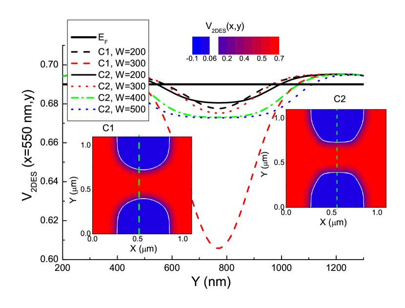
Figure 3: (Color online) Potential profile across the QPCs for two different geometrical patterns. Insets depict the smooth (C1) and the sharp edged (C2) patterns. Dark (blue) regions are electron depleted, i.e. the local potential is larger than the $E_{F}$, denoted by the solid thick horizontal line. White contours denote the depletion boundary, where the width of the QPC is set to be 200 nm and the curvature is changed. The dashed lines stand for the first configuration and two different $W$ values ($=200$ nm (black) and $300$ nm (red)), whereas for the sharper configuration four $W$ values are selected.

The different configurations of the gate patterns are also important when investigating the scattering processes by magnetic focusing experiments Aidala et al. (2007). It is apparent that the scattering patterns of the electron waves will not only depend on the impurity distribution but also on the structure of the QPC’s. We expect that for the sharper defined QPC (C2) the scattering should depend weakly on the QPC opening, since the width does not change along the constraint. Whereas, for C1 configuration small changes at $W$ should affect the scattered waves drastically. Another comment on the experimental setups is to the Roddaro Roddaro et al. (2005) experiments, since the formation of (stable) integer filling region is important to explain Lal (2007) the findings, we believe that C2 type configurations would be leading to a better resolution of the transmission amplitudes. The choice of the structure and the width apparently depends on the experimental interest, which is believed to be irrelevant when modelling QPCs as ideal point contacts, and the QPC’s are not only defined by gates but alternatively also by chemical etching. The gated structures are of course more controllable, however, at high gate voltages required for depletion, electrical sparks can occur, therefore the structure can even be destroyed. In such situations etching defined QPCs are preferred, although without further gates one loses the full control of the potential profile. In the next section, we will compare the potential profiles of etched and gate defined QPC’s, to show that in some cases etch defined QPC’s may be more useful to obtain steeper potential profiles.

II.2 Etching versus gating

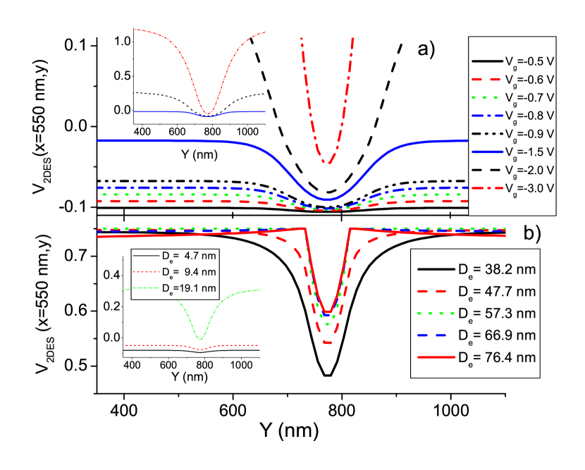
Figure 4: Potential cross-section of (a) gated and respectively (b) etched QPC’s at selected gate biases and etching depths for C1 at a fixed $W=150$ nm. Insets focus on the high bias or shallow etching profiles

For simple calculation purposes, QPCs are modelled either as a finite potential well or with a parabolic confinement potential, perpendicular to the current direction. Starting from the early experiments van Wees et al. (1988), usually the conductance is measured as a function of the applied gate voltage which presents clear quantized values. This quantization can be well explained by the Landauer formula Landauer (1981)

$$G=\frac{e^{2}}{\pi\hbar}\sum_{n,m=1}^{N_{c}}|t_{n,m}|^{2},$$ (2)

where ballistic transport is assumed to take place, i.e. the transmission is given by $|t_{n,m}|^{2}=\delta_{n,m}$, and no channel mixing is allowed. The (integer) number of channels $N_{c}$ is defined by the Fermi energy and the width of the constriction, in general. The gate defined QPCs, at a first order approximation, can be represented by parabolic or finite well potential profiles. However, it is known that the chemical etching process creates (side) surface charges, which in turn generates a steeper potential profile at the edges of the sample. In this situation it is apparent that, the confinement potential can not be assumed to be parabolic, rather a steeper potential should be considered. In this section we compare these two different constriction profiles, namely the gated and the etched ones.

The self-consistent potential across the QPC at the center is plotted versus the lateral coordinate in Fig. 4. The 2DES under the gates is depleted at the gate voltages larger than $-1.5$ V, similarly when the depth of the etching is larger than $47.7$ nm. In both cases, till the depletion is reached the potential profile is varying rather smoothly and the depth of the potential depends linearly on the applied gate bias or the depth. This behavior is drastically changed when electrons are depleted, the potential now strongly depends on the gate potential or depth. Moreover, for the etched structure, potential becomes very steep at the edge of the QPC when $D_{\rm e}>47.7$ nm, i.e. is deeper than the donor layer. The transition from linear behavior to non-linear behavior is simply due to the significant change of the screening properties of the system. Once the electrons are depleted, the external potential can no longer be screened, therefore the amplitude of the self-consistent potential increases by a large amount. Therefore, screening calculations based on the formula given in Eqn. (1) can not account for such situations, where the dielectric function is not aware of the Fermi energy, i.e. the occupancy. A better approximation to this approach is to consider a Linhard type dielectric function, which also takes into account the Fermi momentum Ando et al. (1982). It is known that, such an improvement will also cover some of the quantum mechanical aspects (such as the wave functions), which brings extra oscillations to the potential profile Meir et al. (2002). However, for our present interest we neglect this correction knowing that the self-consistency of the calculation scheme already takes into account the occupation and the 1D electron density at the QPC satisfy the validity condition $n_{\rm el}a_{B}^{*}>>1$ of the TFA Siddiki and Marquardt (2007).

We summarize our findings in Fig. 5, where we show the electron density (left) and potential profiles (right) for typical gate biases $V_{\rm g}$ and etching depths $D_{\rm e}$ versus the spatial coordinate. We choose a representative cross-section of the obtained profiles along the current direction $x$, where the $y$ coordinate is fixed at $450$ nm. Figure  5a depicts the density profile for selected depths of etching varying from shallow ($D_{\rm e}=4.7-19.1$ nm) to deep ($D_{\rm e}=38.2-78.4$ nm). For the smallest two $D_{\rm e}$’s, the 2DES is not depleted beneath the pattern and the density profile is rather smooth. Depletion is observed when the depth is larger than $19.1$ nm, however, until the etching depth reaches to the depth of 2DES ($\sim 60$ nm) we do not see the surface charges (the spike like point, indicated by the arrow) at the level of the 2DES. The inset of Fig. 5b shows the electron density distribution in a color coded contour plot together with the corresponding potential profile across the white (dashed) line. The thin (green) lines contouring the depleted (red) region indicates the spatial distribution of the surface charges. The potential is steeper compared to that of the gated one (Fig. 5d) and the profile does not show any considerable variation once the etching depth reaches the plane of the 2DES. This behavior clearly exhibits the uncontrollability of the etched samples, since the corresponding potential profile obtained for the gated samples vary slowly on the length scales of the Fermi wavelength, even if the 2DES is completely depleted beneath the gates. Moreover, the amplitude of the potential strongly depends on the applied gate voltage. The slow variation of the potential is not the case for the etched sample, for example consider the case when $D_{\rm e}$ is changed from 57.3 to 78.4 nm, and compare it with that of the gated sample when voltage is changed from $-2.0$ V to $-3.0$ V. For the gated sample the potential profile remains still smooth, however, the spatial distribution of the electron density is almost unchanged. Meanwhile, for the deeply etched sample both the electron density and the potential profile are steep and the steepness depends very weakly on the etching depth.

From the above discussion we conclude that, for the gated samples the electron density distribution is weakly effected by the applied gate potential when the depletion is once obtained, meanwhile the potential is smooth and strongly depends on $V_{\rm g}$. For the etched samples, potential profile becomes very steep when the etching depth exceeds the depth of the 2DES, since the (side) surface charges pin the Fermi level at the mesa surface to the mid gap of GaAs forming a Schottky like barrier Siddiki and Gerhardts (2003). We should also note that, at zero bias, more electrons are populated under the gates, which is not the case for the etched samples. As a rule of a thumb, when a steeper potential profile is required one should consider chemical etching where the etching depth is deeper than the electron layer and one should keep in mind that biasing gates with high potential does not necessarily imply that the electron density profile is also changed considerably.

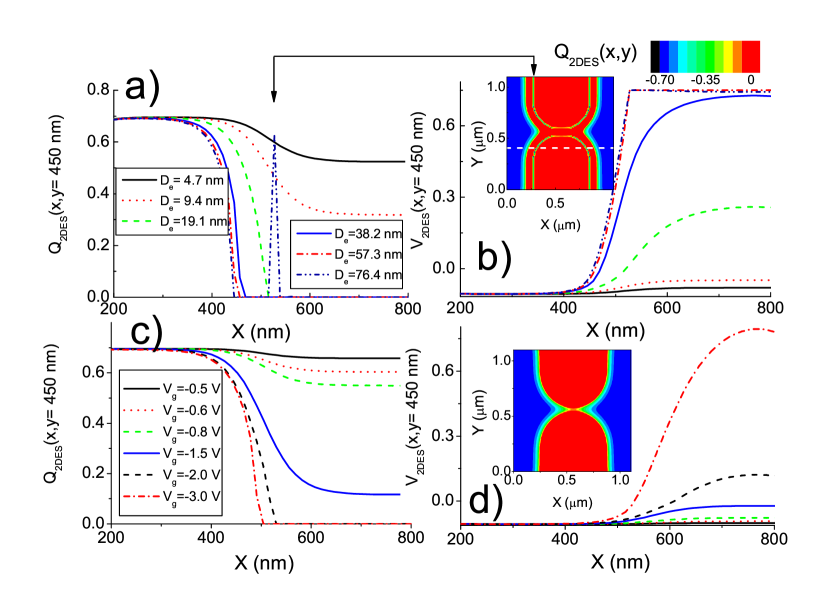
Figure 5: Spatial distribution of the electron density (a,c) and screened potential (b,d) for etched (upper panel) and gated samples (lower panel), $y=450$ nm.

The outcome of the self-consistent solution of the 3D Poisson equation considering QPCs at zero magnetic field is two fold: i) the geometrical properties (i.e. considering C1 or C2 type patterns) strongly change the potential landscape in the close vicinity of the QPCs. We found that the smoother constrictions with a larger width $W$ can be modelled better with the ideal point contacts, i.e. parabolic confinement. The sharper constrictions can be considered as finite well profiles, up to a first order approximation and potential profile remains unchanged when considering $W>300$ nm. ii) Due to surface pinning the etched samples, generate steeper potential profiles and the density profile remains unaffected once etching is deeper than the depth of the 2DES. These numerical results, show a strong deviation from the the widely used ”ideal point contact” and ”frozen charge” models, proposing that depending on the experimental interest it is important to reconsider the geometrical (C1, C2) and structural (gated/etched) factors defining the QPC under investigation. As final remark, the artifacts, such as local minima and maxima at the potential and density profiles, resulting from the previous non-self consistent Thomas-Fermi Siddiki and Marquardt (2007) and ”frozen charge” models Davies and Larkin (1994); Ihnatsenka and Zozoulenko (2007a); Rejec and Meir (2006) are resolved by considering the 3D calculation scheme.

III Finite B Field

The aim of this and the next section is to calculate, and compare, the density and subsequently the current distributions, in the close vicinity of the QPCs, within interacting and non-interacting models in the presence of an external perpendicular magnetic field. Here we take into account electron-electron interaction within the Thomas-Fermi theory of screening also considering strong magnetic fields using the potential profile calculated in the previous section, as an initial configuration of the landscape. We compare the spatial distribution of the Landauer-Büttiker edge states (LB-ES) with the distribution of the incompressible edge states, where the applied external current is confined Chang (1990); Fogler and Shklovskii (1994); Güven and Gerhardts (2003); Siddiki and Gerhardts (2004a). Next we discuss the limitations of the TFA, and suggest improvements on the calculation scheme based on i) quantum mechanical considerations, such as the finite extension of the wave functions, and ii) replacement of the global density of states with the local one.

III.1 Thomas-Fermi-Approximation (TFA)

The enormous variety of the theories describing the density and current distributions at the quantum Hall systems Laughlin (1981); Büttiker (1986); Chang (1990); Chklovskii et al. (1992); Fogler and Shklovskii (1994); Güven and Gerhardts (2003); Siddiki and Gerhardts (2004a) already show the challenge in giving a proper prescription to these quantities. These theories can be grouped into two: the current is carried either (i) by the compressible regions Chklovskii et al. (1992); Beenakker (1989); Büttiker (1988) or (ii) by the incompressible regions Chang (1990); Fogler and Shklovskii (1994); Komiyama et al. (1996); Güven and Gerhardts (2003); Siddiki and Gerhardts (2004a). Moreover (and confusingly) these regions can reside at the bulk Laughlin (1981); Kramer et al. (2003) or at the edge of the sample Büttiker (1988); Chang (1990); Chklovskii et al. (1992); Güven and Gerhardts (2003); Siddiki and Gerhardts (2004a); Kanamaru et al. (2006), depending on the model considered and the magnetic field strength Siddiki and Gerhardts (2004a). For the sake of completeness, we start with a generic Hamiltonian describing an electron subject to high magnetic fields.

$$H^{\sigma}=H_{0}+V^{\sigma}_{\rm int}+V_{\rm ext}+V^{\sigma}_{\rm Z},$$ (3)

where $\sigma(=\pm 1/2)$ is the spin degree of freedom, $H_{0}$ the kinetic part, $V_{\rm ext}$ and $V_{\rm int}$ the external and the interaction potentials, respectively, and $V^{\sigma}_{\rm Z}$ Zeeman term Ihnatsenka and Zozoulenko (2006). Our first assumption is to neglect the spin degeneracy, knowing that the effective band $g-$ factor for the GaAs/AlGaAs hetero-structures is a factor of four less than the one of a free electron gas, and therefore Zeeman splitting is much smaller than the Landau splitting ($\hbar\omega_{c}$, with $\omega_{c}=eB/m^{*}$, i.e. $|g^{*}\mu_{B}B|/\hbar\omega_{c}\approx 0.027$, where $\mu_{B}$ is the Bohr magneton. However, Zeeman splitting can be as large as the Landau splitting if exchange and correlation effects are taken into account at significantly high magnetic fields, hence filling factor $\nu$ ($=E_{F}/\hbar\omega_{c}$) one plateau can be observed experimentally. On the other hand, for higher filling factors $\nu>1$ exchange and correlation effects are assumed to be small and Zeeman splitting is negligible. Thus one can consider spin-less electrons in the magnetic field interval we are interested in, which yields to the effective Hamiltonian,

$$H^{\rm eff}=H_{0}+V_{\rm ext}(x,y)+V_{\rm int}(x,y).$$ (4)

The kinetic part, $H_{0}$, can be solved analytically using the Landau gauge which yield plane wave solutions in one direction ($y$) and Landau wavefunctions in the other direction ($x$). Here, implicitly, a long Hall bar (ideally infinite) is assumed, which is justified while the Fermi wave length is ($\sim 30-40$ nm) much smaller than the sample length under consideration ($L_{y}$ $\sim 1500$ nm). Then the eigenfunctions of $H_{0}$ can be expressed as

$$\Phi_{n,k_{y}}(x,y)=\frac{1}{\sqrt{2^{n}n!\sqrt{\pi}lL_{y}}}\exp{(ik_{y}.y)}\times$$

$$\exp{[-(\frac{x-X}{l})^{2}/2]}\times H_{n}(\frac{x-X}{l}),$$ (5)

where $k_{y}$ is the quasi-continuous momentum in $y$ direction, $n$ the Landau index, $X=-l^{2}k_{y}$ a center coordinate, and $H_{n}(\xi)$ the $n$th order Hermite polynomial with the argument $\xi$, whereas the eigen energies are

$$E_{n}=\hbar\omega_{c}(n+1/2).$$ (6)

The essence of the TFA relies on the fact that the potential profile varies smoothly on the quantum mechanical length scales. Through out this work we will only consider the $6-8$ T interval and as a rough estimation the extend of the wavefunctions in $x$ direction (of the ground state, i.e. $\nu=2$), or the magnetic length $l=\sqrt{\hbar/m\omega_{c}}$, will be always similar or less than $10$ nm, therefore in almost all cases neglecting the finite extend of the wavefunctions is still reasonable. However, we have already seen that for the etched samples the potential is quite steep and the results obtained from the TFA may be doubted, which we will address in the next section.

At the moment let us consider a case that the condition of TFA holds, i.e. the total potential $V_{\rm tot}(x,y)=V_{\rm ext}(x,y)+V_{\rm int}(x,y)$ varies smoothly on the quantum mechanical length scales and the sample is long enough (i.e. $k_{F}L_{y}\gg 1$). Then we can replace the wavefunctions in both directions by wave packets centered at $X$, and at $y$ and the center coordinate dependent eigenenergy $E_{n}(X)$ can be approximated to $E_{n}+V_{\rm tot}(X,y)$. It follows that the spatial distribution of the electron density within the TFA is given by the expression  Lier and Gerhardts (1994); Siddiki and Marquardt (2007); Siddiki et al. (2008a),

$$n_{\rm el}(x,y)=\int D(E,(x,y))f(E+V_{\rm tot}(x,y)-\mu^{*})dE$$ (7)

with $D(E,(x,y))$ (local) density of states, $f(E)=1/[\exp(E/k_{b}T)+1]$ the Fermi function, $\mu^{*}$ the electrochemical potential, which is a constant in equilibrium state, $k_{B}$ the Boltzmann constant, and $T$ the temperature. Once the electron density is obtained, the interaction potential, i.e. the Hartree potential, can be obtained from

$$V_{\rm int}(x,y)=\frac{2e^{2}}{\bar{\kappa}}\int_{A}K(x,y,x^{\prime},y^{\prime})n(x^{\prime},y^{\prime})dx^{\prime}dy^{\prime}.$$ (8)

Here, $\bar{\kappa}$ is an average dielectric constant ($=12.4$ for GaAs) and $K(x,y,x^{\prime},y^{\prime})$ is the solution of the 2D Poisson equation satisfying the boundary conditions dictated by the sample. The results reported in this and the following section assume periodic boundary conditions, where a closed form of the kernel $K(x,y,x^{\prime},y^{\prime})$ can be obtained analytically Morse and Feshbach (1953). Equations (7) and (8) form a self-consistent loop to obtain the potential and the density profiles of a 2DES subject to high perpendicular magnetic field in the absence of an external current at equilibrium, which has to be solved iteratively using numerical methods. The computational effort to calculate electron and potential profiles within the TFA is much less than that of the full quantum mechanical calculation procedures. The results of both agree quantitatively very well in certain magnetic field intervals where the widths of the incompressible strips $W_{\rm IS}$ (in which the potential changes strongly) is larger than $l$. If $W_{\rm IS}\lesssim l$ condition is reached, first of all the TFA becomes invalid and the calculation of the electron density should include the finite extend of the wavefunctions. The underestimation of the quantum mechanical effects lead to existence of artificial incompressible strips both in the non self-consistent electrostatic approximation (NSCESA) Chklovskii et al. (1992, 1993) and self-consistent TFA schemes Oh and Gerhardts (1997); Siddiki and Gerhardts (2003). In fact, as early as the NSCESA, the self-consistent schemes which also took into account finite extend of the wave functions already pointed out the suppression of the incompressible strips in certain magnetic field intervals Suzuki and Ando (1993) and also in the recent reports Siddiki and Gerhardts (2004a); Ihnatsenka and Zozoulenko (2006). For a systematic comparison of the calculated widths of the incompressible strips within the TFA and the full Hartree approximations, we suggest the reader to check Ref. [Siddiki and Gerhardts, 2004a], where a simpler quasi-Hartree scheme is proposed to recover the artifacts arising from TFA.

III.2 Corrections to the TFA

Historically, the first implementation of the TFA, including electron interactions, to quantum Hall systems goes back to the seminal work by Chklovskii et.al Chklovskii et al. (1992). There it was shown that within the electrostatic approximation the 2DES is divided into two regions which have completely different screening properties. In this model, a translation invariance is assumed in the current ($y-$) direction. Due to finite widths of the samples in the $x$ direction the electrostatic potential is bent upwards at the edges of the sample, hence the Landau levels, $E_{n}(X)=E_{n}+V(X)$. Inclusion of the Coulomb interaction and the pinning of the Fermi energy to the Landau levels result in two regions (strips): i) The Fermi energy is pinned to one of the highly degenerate Landau levels, then the screening is perfect, effective potential is completely flat (metal like) and electron density varies spatially ii) The Fermi energy falls in between two consecutive Landau levels, screening is poor, effective (screened) potential varies (the amplitude of the variation is $\hbar\omega_{c}$) and electron density is constant over this region. It is apparent that, if the potential varies rapidly on the scale of $l$, the TFA fails and the results become unreliable. This condition is realized when considering narrow incompressible strips having a width smaller than the magnetic length. Therefore, one should include the effect of wave functions within these narrow strips. One way is, of course, to do full Hartree calculations. We already mentioned the challenges in the computational effort. A simpler approach is to replace the delta wave functions of the TFA with the unperturbed Landau wave functions, i.e. quasi Hartree approximation Siddiki and Gerhardts (2004a)(QHA). The findings of the QHA is shown to be more reasonable than of the TFA, which now also includes the finite extend of the wave functions in the close vicinity of the incompressible strips. Therefore, as an end result, when the $W_{\rm IS}\lesssim l$ condition is reached the incompressible strip disappear due to the overlap of the neighboring wave functions. Based on this fact, in our calculations in the following we will exclude the effects arising from the artifacts of the TFA by considering a spatial averaging of the electron density on the length scales smaller than $l$, which is known to be relevant in simulating the quantum mechanical effects Siddiki and Gerhardts (2007); Siddiki et al. (2006); Siddiki (2007).

We should also make one more point clear that with the NSCESA usually a gate defined quantum Hall bar is considered. It is more common to define Hall bars by chemical etching and the edge potential profile is much more steep compared to gated samples which was shown in the previous section. Therefore, to fit the predictions of this model concerning the widths and the positions of the incompressible strips with the experimental data one has to assume that Ahlswede et al. (2001) i) the 2DES and the gates are on the same plane and ii) the gate voltage applied should be fixed to the half of the mid gap of the GaAs, i.e. pinning of the Fermi energy at the GaAs surface. In fact, after making these two crucial assumptions the experimental findings of E. Ahlswede Ahlswede et al. (2001) perfectly fits with the NSCESA. However, the widths (and the existence) of the incompressible strips strongly deviate from the predictions, since only the innermost incompressible strip can be observed. We have argued that, the widths of the incompressible strips strongly depend on the slope of the potential, i.e. if the external potential is steep the incompressible strips are narrow. Therefore one can easily conclude that, since the widths of the outermost incompressible strips become smaller than the magnetic length, the outer incompressible strips, i.e. the ones close to the edge, disappear and could not be observed. The overestimation of the $W_{\rm IS}$ within the TFA becomes more severe when an external current is imposed to the system, which we will discuss in the next section. Before discussing the results of the relaxed TFA, we want to touch another locally defined quantity, namely the DOS, and comment on the implementation of the global DOS to our local TFA.

In the absence of impurity scattering the DOS of an infinite (spin-less) 2DES is given by the bare Landau DOS as

$$D(E)=\frac{1}{2\pi l^{2}}\sum_{n}{\delta(E-E_{n})}$$ (9)

however, this DOS is broadened by the scattering processes, which can be described in self-consistent Born approximation Ando et al. (1982); Siddiki and Gerhardts (2004a) accurately for short range impurity potentials yielding a semi elliptic broadening. Of course, other impurity models and scattering processes can also be considered resulting in Gaussian or Lorentzian broadened Landau DOS Güven and Gerhardts (2003); Eksi et al. (2007). In such descriptions of the DOS broadening an infinite 2DES is assumed and the DOS is calculated for impurity distributions averaged over all possible configurations. Inserting this (global) DOS in Eqn. (7) can be justified again if the TFA condition is satisfied. We have already shown that this condition is violated when a narrow incompressible strip is formed where the external potential is poorly screened. Therefore, the actual distribution of the impurity potential becomes more effective at these transparent regions. We should also note that the effect of screening on the DOS of an infinite system has been investigated in detail in Ref. [Cai and Ting, 1986] and it has been shown that, since the screening is poor within the incompressible regions, the DOS becomes much broader than that of the non-interacting case. Hence, the gap between two consecutive Landau levels is narrower within the incompressible strips compared to compressible strips. Moreover, recently it has been shown that the (local) electric field within the sample also leads to broadening of the (local) DOS Kramer (2006). The idea is basically that one calculates the Greens function for the given potential profile, which is a function of the applied magnetic field and external current, and obtains the local DOS from the general expression

$$D(E,(x,y))=\sum_{n}{|\widetilde{\Phi}_{n,k_{y}}(x,y)|^{2}\delta(E-\widetilde{E}_{n,k_{y}})},$$ (10)

where $\widetilde{\Phi}_{n,k_{y}}(x,y)$ is the $n$th eigenfunction of the Hamiltonian given at Eqn. (4) with the eigenvalue $\widetilde{E}_{n,k_{y}}$. In our above discussion about the formation of the compressible/incompressible strips we have mentioned that the potential varies locally whenever an incompressible strip is formed, where the variation is linear in position up to a first order approximation. Now let us consider a linear potential profile and re-obtain the local DOS (LDOS) following Kramer et al. (2004) for the $k$th Landau level,

$$D_{k}(E)=\frac{1}{2^{k+1}k!\pi^{3/2}l^{2}\Gamma}e^{-E^{2}_{k}/\Gamma^{2}}[H_{k}(E_{k}/\Gamma)]^{2}$$ (11)

with the level width parameter

$$\Gamma=\mathcal{E}_{x}l$$ (12)

where $\mathcal{E}_{x}=\partial{V(x,y)}/\partial{x}$ is the electric field in the $x$ direction and $E_{k}=E-\Gamma^{2}/(4\hbar\omega_{c})+(2k+1)\hbar\omega_{c}$. The immediate consequence of a strong electric field in the $x$ direction is a broadening of the LDOS, which happens at the incompressible strips. On the other hand, since $\mathcal{E}_{x}$ vanishes at the compressible strips, the bare Landau DOS is reconstructed from Eqn. (11) in the $\Gamma\rightarrow 0$ limit.

In summary, the TFA should be repaired when the widths of the incompressible strips is comparable or less than the magnetic field, since (i) the quantum mechanical wave functions have a finite extend and do overlap with the neighboring ones (ii) the LDOS are broadened where strong electric fields exist, (iii) within the poor screening regions the (Landau) gap is smaller than the ones of the nearly perfect screening regions. At the very simple approximation this artefact of TFA is cured by a spatial averaging over the Fermi wavelength resulting in nonexistence of narrow incompressible strips. In the following an appropriate averaging process will be applied.

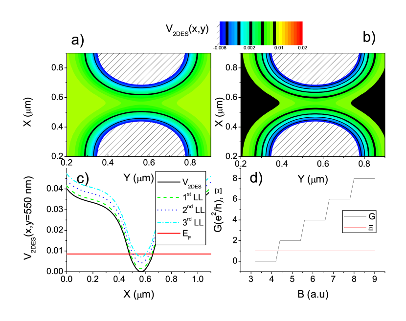
Figure 6: The distribution of the spin degenerate LB-ES at (a) $\nu\approx 4$ and (b) $\nu\approx 8$. The potential cross-section at $\nu=8$ plateau (c). Sketch of the conductance (G) and expected coherence $\Xi$ (d) for C1 considering $W=150$ nm with an applied gate potential $V_{g}=2.0$ V, so that the 2DES is depleted beneath the gates. Since spin degeneracy is assumed each edge state carries two units of quantized current.

III.3 Results

The transport through the QPCs in the absence of an external magnetic field is well described by the Landauer formalism, summarized in Eqn. (2). The main idea is that the transport is ballistic and due to the cancellation of the velocity and a 1D DOS Davies (1998), the conductance is integer multiples of the conductance unit, $e^{2}/h$. These integers are just the number of channels $N_{c}$, i.e. the number of eigen energies below the Fermi energy. A similar path is followed when considering an external $B$ field, which assumes that the conductance is ballistic within 1D channels and neglects the electron interactions. These 1D channels are formed whenever the Fermi energy coincides with a Landau level (Landauer-Büttiker picture). Before proceeding with the full self-consistent solution of the density and current distribution problem, we first investigate the positions of the Landauer-Büttiker edge states. The procedure is simple, to obtain the energy dispersion we use the relation

$$E_{n,k_{y}}(x,y)=E_{n}+V(x,y)$$ (13)

and follow the equipotential (energy) lines coinciding with the Fermi energy. By doing so we would be able to discuss qualitatively the phase coherence $\Xi$, taken to be equal to 1 when there is a full phase coherence and 0 when there is none. We neglect all the external sources of decoherence and assume that the LB-ES are coherent at the length scales we are interested in, i.e. the wave functions of the associated channels do not overlap.

In Fig. 6, we show the spatial distribution of the expected positions of the LB-ES at two filling factors. The color scale depicts the self-consistent potential, whereas the black strips show the LB-ES. The white shaded areas are the electron depleted regions. The $\nu=2$ and $\nu=4$ edge states nicely show the expected distribution which are spatially $\sim 40$ nm apart, Fig. 6a. Depending on the steepness of the potential or the magnetic field value, however, this distance may become less. For the etched samples (not shown) at the same filling factor the spatial distance between $\nu=2$ and $\nu=4$ edge states become almost half the value of the gated samples. For a filling factor $\nu=$8 plateau the outermost (the ones closest to the gates) two edge states are less than 15 nm apart from each other, and the wave functions extend over a larger distance. It is apparent that, when the two wave functions start to overlap, the coherence $\Xi$ is reduced drastically. However, for the ideal case (no overlap) $\Xi$ should stay constant for all plateau regions, since by definition the edge states can not cross each other. The conductance quantization is, of course, independent of the structure of the ES itself and according to Eqn. (2) one should simply count the number of ES which cross the constriction. The conductance is shown by the sketch in Fig. 6d, of course the sharp transition between the plateaus is changed when one considers level broadening or in general scattering. One should note that, although the LBES picture is useful in making qualitative arguments, one needs to grasp the actual distribution of the edge states to understand the physics observed at the experiments Litvin et al. (2008).

Next we investigate the distribution of the incompressible strips calculated self-consistently described by Eqns. (7-8). The conductance through the QPC can be rewritten

$$G=\frac{e^{2}}{h}\nu_{\rm center}$$ (14)

as conjectured in Ref. [Chklovskii et al., 1993], where $\nu_{\rm center}$ is the filling factor at the very center of the QPC. It is apparent that, if this value is an integer, i.e. incompressible, the conductance is quantized. Therefore, it is important to study this condition for a realistic QPC geometry. In the following we first calculate the filling factor distribution in the absence of an external current and then obtain the current distribution in the next section.

In order to cure the artifacts arising from TFA i) we consider a DOS broadened by a Gaussian Güven and Gerhardts (2003)given by

$$D(E)=\frac{1}{2\pi l^{2}}\sum_{n=0}^{\infty}\frac{\exp(-[E_{n}-E]^{2}/\Gamma_{\rm imp}^{2})}{\sqrt{\pi}\,\Gamma_{\rm imp}}$$ (15)

with the impurity parameter $\Gamma_{\rm imp}$, which is chosen large enough $\Gamma_{\rm imp}/\hbar\omega_{c}=0.3$ to cover the level broadening generated by the local electric field Kramer et al. (2003) and self-consistent broadening effects Cai and Ting (1986) and ii) a spatial averaging is carried out over the Fermi wavelength ($\sim 30$ nm). Fig. 7 summarizes our results showing the spatial distribution of the incompressible ES, considering the quantum Hall plateau $\nu=2$. Pedagogically, starting our investigation from large magnetic fields is preferable; at large magnetic fields (Fig. 7e), the system is mostly compressible (colored area) and the two incompressible (white) regions do not merge at the opening of the QPC. Therefore, both the Hall resistance and the conductance through the QPC is not quantized. As soon as one enters to the QH plateau almost all of the sample becomes incompressible shown in Fig. 7d (in the absence of short range impurities) and both $R_{H}$ and $G$ becomes quantized. Decreasing the magnetic field creates two incompressible ES which are spatially separated seen in Fig. 7b, however, the quantization is not affected. At a lower magnetic field value these IS-ES disappear (Fig. 7a) as an end result of level broadening and (simulation) of the finite extend of the wave functions, now we are out of the QH plateau and G is no longer quantized. This picture and the LB-ES picture yield same behavior for the $R_{H}$ and $G$, however, in the later one current is carried by the IS-ES, which we will discuss in the next section. The qualitative difference between the two pictures is the coherence as shown by the (red) dashed line in Fig. 7c. First $\Xi$ presents minima in between two plateau regimes, since the IS die out, second at the higher edge of the QH plateau the system becomes completely incompressible therefore, it is not possible to define separate ESs hence coherence is lost (averaged). We believe that, this nonuniform behavior of the coherence within the QH plateau coincides with the experimental findings of Roche et.al. Roulleau et al. (2007b), however, we admit that other explanations are also possible. Another interesting experimental work is carried by the Regensburg group, where they have investigated the amplitude of the visibility oscillations as a function of $B$ field Litvin et al. (2008). They have reported a maximum visibility at $\nu\thickapprox 1.5$, which seems quite opposite to, what has been reported by other groups Ji et al. (2003); Roulleau et al. (2007b). However, it is easy to see that their sample has a homogeneous width all over, which is not the case for other groups. From self-consistent calculations Siddiki and Gerhardts (2007) it known that, if the sample width is narrower than 5-6 $\mu$m the center electron density (or filling factor) can differ strongly from that of the average one(s). An indication of such a case is also shown by numerical simulations Siddiki et al. (2008b).

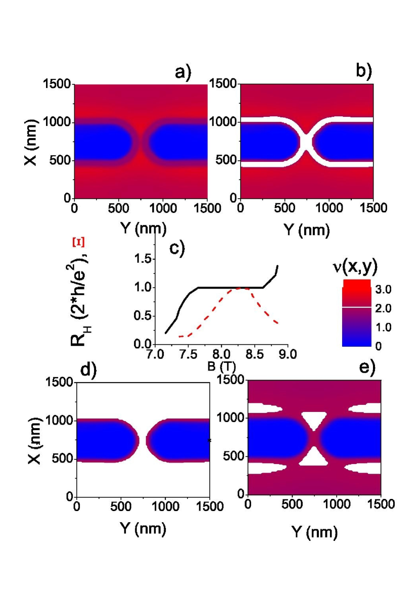
Figure 7: Spatial distribution if the incompressible strips (white areas) for characteristic $B$ values (a) 6.8 T, (b) 7.3 T, (d) 8.3 T (e) 8.8 T calculated at temperatures $\hbar\omega_{c}/k_{B}T\ll 1$, together with the sketch of Hall resistance and the coherence $\Xi$ (c). The QPC configuration considered here is C1 with $W=150$ nm, the gate voltage is chosen such that all the electrons beneath the gates are depleted.

In interconnecting the Hall plateaus and the spatial distribution of the incompressible strips, we have used the findings of Ref. [Siddiki and Gerhardts, 2004a] where the current is shown to be flowing through the incompressible strips. This is in contrast to some of the models Chklovskii et al. (1992); Beenakker (1989) in the literature where the opposite is proposed. In the next section, we will present the general concepts of the local Ohm’s law and based on the absence of back scattering in the incompressible strips we will show that the local resistivity vanishes and the external current should be confined to these regions.

IV Current distribution within local Ohm’s law

The local (potential) probe experiments Ahlswede et al. (2001, 2002); Ilani et al. (2000), brought novel information concerning the Hall potential distribution over the sample. The first set of experiments show clearly that the potential, therefore the current, distribution is strongly magnetic field dependent. It was shown that, out of the QH plateau regime the Hall potential varies linearly (Type I) all over the sample, a similar behavior to classical (Drude) result. Whereas, at the lower edge of the QH plateau the current is confined to the edges of the sample (Type II), which was shown to be coinciding with the positions of the incompressible strips. The most interesting case is observed when an exact (even) integer filling is approached. In these magnetic field values, the potential exhibits a strong nonlinear variation all over the sample, which was attributed to the existence of a large (bulk) incompressible region. The explanation of these measurements acquired a local transport theory, where the conductivities and therefore current distribution can be provided also taking into account interactions. In the subsequent theoretical works Güven and Gerhardts (2003); Siddiki and Gerhardts (2004a, b) the required conditions were satisfied and an excellent agreement with the experiments were obtained Ahlswede et al. (2001). In the second set of experiments Ilani et al. (2004) a single electron transistor has been placed on top of the 2DES and the local transparency, i.e. whether the system is compressible or incompressible, and the local resistivity have been measured. Comparing the transparency and the longitudinal resistivity, it has been concluded that the resistivity vanishes when the system is incompressible.

Theoretically, if the local electrostatic potential and the resistivity tensor $\hat{\rho}(x,y)$ are known the current distribution $\vec{j}(x,y)$ can be obtained from the local version of the Ohm’s law

$$\vec{E}(x,y)=\hat{\rho}(x,y).\vec{j}(x,y)$$ (16)

provided that

$$\vec{E}(x,y)=\nabla\mu^{*}(x,y)/e$$ (17)

where the electrochemical potential is position dependent when an fixed external current $I=\int_{A}{\vec{j}(x,y)dxdy}$ is imposed. In our calculations we assume a local equilibrium in order to describe the stationary non-equilibrium state generated by the imposed current, starting from a thermal equilibrium state obtained from the modified TFA. At this point if the local resistivity tensor is known, Eqn.s (16)-(17) should be solved once again iteratively for a given electron density and potential profile, where the equation of continuity

$$\bf{\nabla}\cdot\textbf{j}(\textbf{r})=0$$ (18)

also holds. We assume that the local resistivity is related to the local electron density via the conductivity tensor, i.e. $\hat{\rho}(x,y)=\hat{\sigma}^{-1}(n_{\rm el}(x,y))$. For a Gaussian broadened DOS the longitudinal component of the conductivity tensor is obtained from

$$\sigma_{l}=\frac{2e^{2}}{h}\int_{-\infty}^{\infty}dE\large[-\frac{\partial f}{\partial E}\large]\sum_{n=0}^{\infty}\large(n+\frac{1}{2}\large)[e^{(-[\frac{E_{n}-E}{\Gamma_{\rm imp}}]^{2})}]$$ (19)

whereas Hall component is simply

$$\sigma_{H}=\frac{2e^{2}}{h}\nu,$$ (20)

where we ignored the self-energy corrections depending on the type of the impurity scatterers. We should emphasize that, the above conductivities are used for consistency reasons, in principle, any other reasonable impurity model like the commonly used SCBA Ando et al. (1982); Siddiki and Gerhardts (2004a) can be considered. Assuming that TFA is valid, we can replace the local conductivities with the above defined global ones.

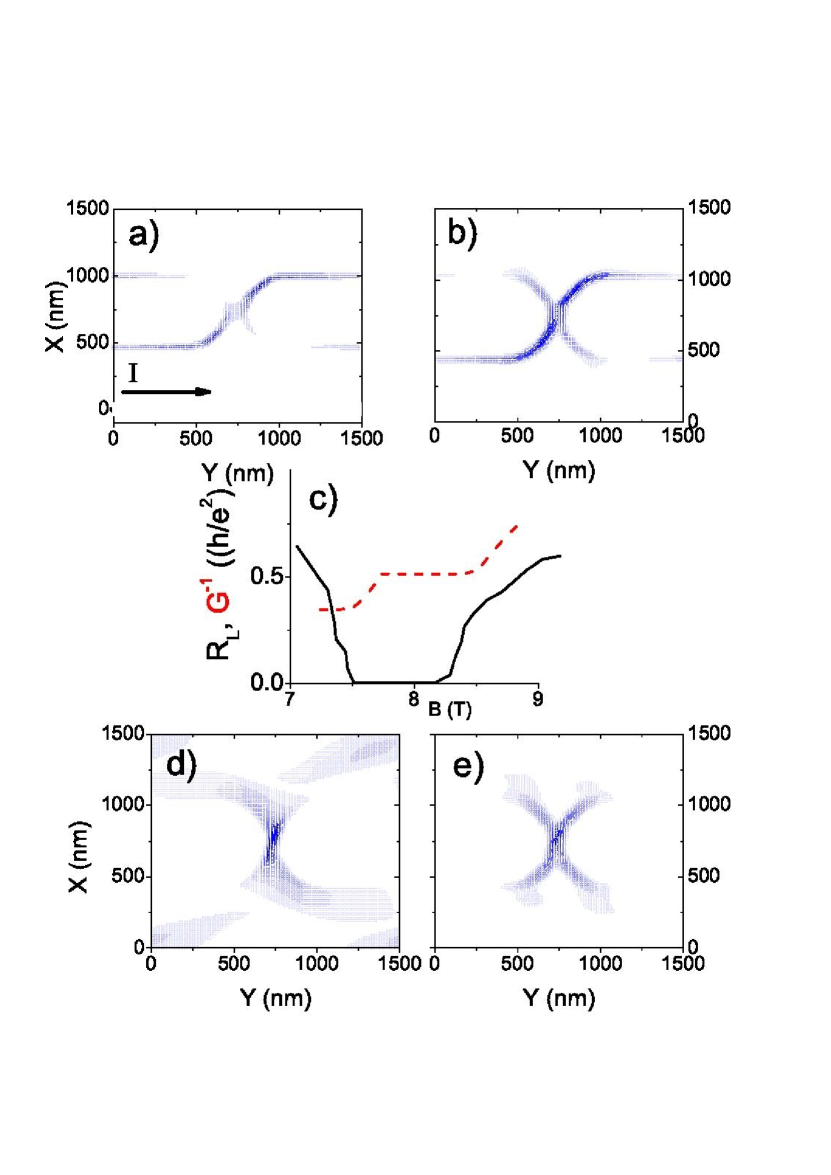
Figure 8: The local current density calculated at different field strengths, same as in Fig.7. The intensity of the current density is chosen such that, the applied current does not effect the density distribution, i.e. $|j(x,y)|\sim 0.4\times 10^{-3}$ A/m.

In the absence of an external current our calculation scheme is as follows, we initialize Eqn. (7) using the total potential obtained from the 3D calculations and obtain the electron density at relatively high temperatures ($kT/\hbar\omega_{c}\sim 0.5$) and use this density distribution to obtain resulting potential from Eqn. (8). Next we keep on iterating until a numerical convergence is reached, where the electron density is kept constant. This is followed by the step where the temperature is lowered by a small amount and iteration process is repeated till the target temperature is reached. After the thermal equilibrium is obtained, we impose a small amount of external current and solve Eqns. (16-17) self-consistently. While doing this second iteration, we fix the constant arising from the integral equation to a value such that the total number of electrons is kept constant with and without current. As a numerical remark, if the current loop does not converge we increase the temperature by a relevant amount and start the iteration procedure. The whole calculation scheme is composed of three different codes, which are written in C++, Fortran and Matlab respectively. In order to obtain reasonable grid resolution parallel computation techniques were used Arslan (2008).

Since we are interested in current distribution and also its effect on the density distribution we find appropriate to present our results in two separate sections i) where the applied current is weak enough that the electron and potential distribution is unaffected, linear response. ii) the applied current is sufficiently large so that the imposed current induces a considerable change on the position dependent electrochemical potential, out of linear response.

IV.1 Linear response regime

The crucial part of the local approach is that for a given (large) magnetic field we can calculate the local potentials and electron distributions self-consistently. The result of such a calculation is that the 2DES is essentially separated in two regions, i.e. compressible and incompressible, therefore for a given (obtained) density we can calculate the local conductivities via Eqns. (19-20). Let us now discuss the distinguishing conductance properties of these two regions starting from a compressible region. At a compressible region the Fermi energy is pinned to one of the Landau levels, screening is nearly perfect, self-consistent potential is flat and filling factor is locally a non-integer. According to Eqn.(20), the Hall conductivity is a non-integer and the longitudinal conductivity is non-zero meaning finite back scattering. Now the classically defined drift velocity, and also its quantum mechanical counter part, is proportional to the electric field perpendicular to the current direction. We have seen that at the compressible region the potential perpendicular to the current direction is flat, therefore the $x$ component of the electric field is zero, hence the drift velocity. Meanwhile, at an incompressible region the Fermi energy is in between two Landau levels, the filling factor is fixed to an integer value and potential presents a variation perpendicular to the current direction. Due to the Landau gap the longitudinal conductivity vanishes, whereas the Hall conductivity assumes its (quantized) integer value. If one calculates the inverse of the conductivity tensor for the longitudinal component one obtains,

$$\rho_{l}(x,y)=\frac{\sigma_{l}(x,y)}{\sigma^{2}_{l}(x,y)+\sigma^{2}_{H}(x,y)}$$ (21)

thus the longitudinal resistivity vanishes within the incompressible region pointing the absence of back scattering. Of course, the simultaneous vanishing of both the longitudinal resistivity and the conductivity is a result of applied external (and perpendicular) $B$ field and is obtained only in two dimensions. Moreover, since the $x$ component of the electric field is now non-zero, the drift velocity is finite and the current is confined to this region. Combining these two one concludes that, if there exists an incompressible region somewhere in the sample all the external current is confined to this region otherwise (if there are no incompressible regions and all the system is compressible) the current is distributed according to Drude formalism, i.e. the current density is proportional to the electron density.

We start our discussion of the current distribution when a small current is imposed for which the electrostatic and electrochemical potential satisfies the linear response relation

$$V((x,y);I)-V((x,y);0)\approx\mu^{*}((x,y);I)-\mu^{*}_{\rm eq}.$$ (22)

This condition essentially states that, the imposed current does not modify the electrochemical potential therefore the electron density remains unchanged. Fig. 8 presents the current distribution which is calculated for the density distribution shown in Fig. 7. The correspondence between the positions of the incompressible strips and the current density is one to one. In the out of plateau regime the current is essentially distributed all over the sample, where no incompressible regions exist, Fig.8a. As soon as one enters the QHP, i.e. when a large bulk incompressible strip (region) is formed, the essential future of current distribution is not effected strongly, however, in this situation current is flowing in the incompressible region. Tracking the positions of the ISs in Fig. 7b, we can readily guess the distribution of the current density in Fig. 8b. Following our arguments about the smearing out of the narrow incompressible strips, we have a situation in which, again, the current is spread over the sample shown in Fig. 8a. Although, the IS vanishes the reminiscence of it still provides a narrow strip of small longitudinal resistivity and, therefore a higher amount of current is kept confined to these regions. Fig. 8c, presents the corresponding longitudinal resistance, when measured as a function of $B$ together with the conductance across the QPC. The relation between $G$ and $R_{L}$ is interesting, the conductance is quantized, as soon as $R_{L}$ vanishes at large fields, however, becomes non-quantized even though the $R_{L}=0$ at the lower edge of the zero resistance state. Let us first discuss the $B$ dependence of the $R_{L}$, it is finite if the system is compressible and is zero if an incompressible strip percolates from one edge of the sample to the other edge in the current direction, i.e. from source to drain. Therefore, existence of an IS percolating is sufficient enough to measure zero longitudinal resistance. However, to have a conductance quantization the center of the QPC should be incompressible, which is a stronger restriction Chklovskii et al. (1993). Hence, in the lower edge of the QHP, the IS percolates but the center of the QPC is compressible. The implication of this fact to the coherence is a bit more complicated, we have seen that as soon as one enters to the QHP a large bulk IS is formed therefore the phase of the electrons is highly averaged. This implies that the coherence is relatively less than that of the two well separated ISs. On the other hand, at the lower edge of the conductance plateau, the ISs become narrower and are less immune to decoherence effects arising from the environment, hence, the coherence is reduced. Our above discussion coincides with the recent experiments performed in small Mach-Zehnder interference devices (MZI), where the visibility is measured as a function of the external magnetic field Roulleau et al. (2007b). It is fair to note that, some other mechanisms providing $B$ dependence of decoherence can also account for such a behavior.

In the mentioned MZI experiments Ji et al. (2003); Neder et al. (2006) and also the measurements performed at the group of S. Roddaro Roddaro et al. (2005) a finite (and large) source drain voltage $V_{\rm SD}$ is applied either to measure the $V_{\rm SD}$ dependency of the visibility or the transmission. The intensity of the applied current, in these experiments, can not be treated within the linear response regime, where the electrochemical potential remains constant, i.e. position independent. In the next section, we present the current and the density distribution calculated where Eqn. (22) does not hold any more.

IV.2 Beyond linear response

In the absence of an external current an equilibrium state is obtained by solving the Eqns. (7) and (8) self-consistently. Even in the presence of a small current, a Hall potential is generated which, in principle, modifies the electrochemical potential, i.e. tilts the Landau levels. This modification can be compensated by the redistribution of the electrons, which certainly modifies the total electrostatic potential. If the applied current is sufficiently small, the modification is negligible, i.e. linear response. However, if the current is large, the resulting Hall potential is also large and one should re-calculate the electron density, and therefore the potential distribution till a steady state is reached. In this section we present the current and density distribution in the presence of a large external current, where a local equilibrium is assumed implicitly.

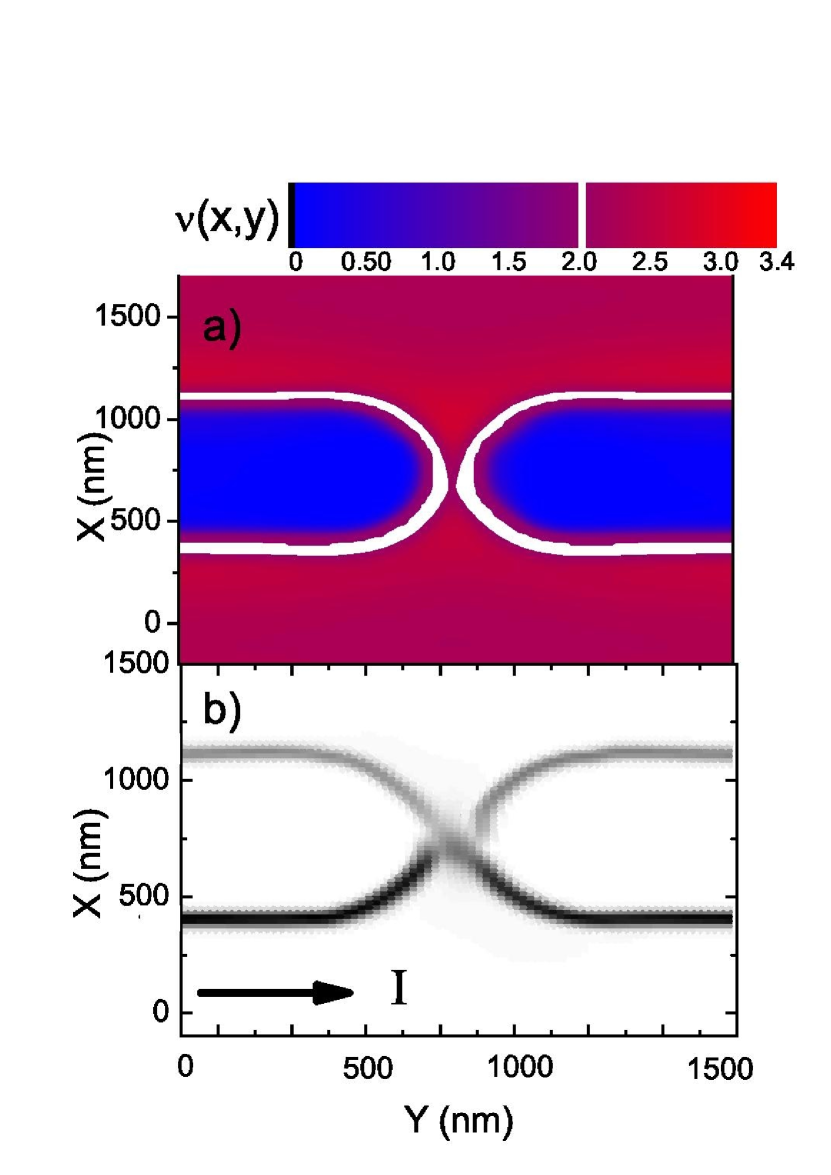
Figure 9: The local filling factor distribution and the corresponding local current density calculated at the default temperature. The current intensity is sufficiently high ($|j(x,y)|=2.0\times 10^{-2}$ A/m) to induce an asymmetry on the density distribution via position dependent electrochemical potential.

Fig. 9a shows the electron density distribution in color scale for $B=7.1$ T, where the intensity of the applied current is in the out of linear response regime. Note that the $B$ value is chosen such that the Hall resistance is quantized, however, the conductance is not. The general behavior is similar to that of linear response, however, it is clearly seen that the widths of the ISs are asymmetric with respect to $y=750$ nm line, where current is driven in $y$ direction. The asymmetry is induced by the large current, since the electrons are redistributed according to the new (self-consistent) potential distribution. The corresponding current density distribution is plotted in Fig. 9b, once more the one to one correspondence between the positions of the ISs and the local current maxima is apparent. The consequence of the asymmetry and thereby the widening of the ISs can be observed in the conductance and the $R_{L}$, such that the narrow IS at the upper side is smeared out much earlier than the one on the lower side. We should note that, such large currents heat the sample therefore the local temperature within the ISs is larger compared to the lattice temperature due to Joule heating Akera (2001). Such a (local) temperature dependence is treated explicitly by H. Akera Kanamaru et al. (2006) and his co-workers and a strong evidence is provided towards explaining the breakdown of the IQHE within this approach. Our present approach lacks such a treatment, therefore the competition between the widening of the ISs and heating due to large currents is thought to be more complicated than presented here. As a consequence, the discussion of the coherence is far beyond our model, however, we think that the amplitude of the current when measuring visibility Roulleau et al. (2007b)] is assumably still in the linear response regime.

In conclusion, by exploiting the local equilibrium and the properties of a steady state we have calculated the current distribution near a QPC in the out of linear response regime. We have shown that a asymmetry is induced on the density profile due to the bending of the Landau levels generated by the large Hall potential. We estimate that, the system can still be considered in the linear response regime if the 1D current density is smaller than $0.042\times 10^{-2}$ A/m, which certainly depends on the details of the sample geometry.

V Summary

In this paper, we provided a self-consistent scheme to obtain the electron density, potential profile and current distribution in the close vicinity of a QPC, within the Thomas-Fermi approximation. Starting from a lithographically defined 3D sample, we calculated the charge distribution at the surface gates, at the plane of 2DES and for etched samples at the side surfaces. The 3D self-consistent solution of the Poisson equation enabled us to present the similarities and differences between an etched and gate defined QPC. We found that, the relatively deep etched samples present a sharp potential profile near the edges of the sample. If the depth of the etching exceeds the depth of the 2DES, surface charges are calculated explicitly. In the presence of a quantizing perpendicular magnetic field, we have calculated the distribution of the incompressible strips as a function of the field strength. We have argued that, if an incompressible strip becomes narrower than the magnetic length and/or if the transverse electric field is sufficiently large, due to Level broadening, the narrow incompressible strip is smeared. In the next step, the current distribution is obtained both in the linear response and out of linear response regimes using a local version of the Ohm’s law assuming a steady state at local equilibrium. It is shown that the current is confined to the incompressible strips, due to the absence of back scattering, otherwise is distributed all over the sample. We have commented on the relation between the existence and percolation properties of the incompressible strips and the measured quantities such as the longitudinal resistance and conductance across the QPC. For the ideal clean sample, i.e. in the absence of long range fluctuations, it is shown that the QH plateau extends wider than that of the conductance plateau. In the out of linear response regime, a current induced density asymmetry is presented for the first time in such geometries under quantized Hall conditions. The observable effects of such an asymmetry are not clarified, since it is also know that large currents increase the temperature locally due to Joule heating.

A natural extension of the existing model is to include the spin degree of freedom and thereby exchange and correlation effects Pittalis et al. (2007). A local spin density functional theory approach Ihnatsenka and Zozoulenko (2007a, b) is the much promising one among others such as Monte Carlo Räsänen et al. (2003) and exact diagonalization, from computational and application point of view. In fact, such an approach already exists, however, the current is handled within the Landauer-Büttiker formalism, which we think is not reasonable in the presence of large incompressible strips. On the other hand, a time dependent spin density functional model would be a good candidate to describe current for the geometries under investigation. The implementation of the Akera’s theory, i.e. Joule heating, to our model is of course desirable which is been worked presently.

Finally, in order to have a predictive power on the interference experiments we would like to utilize the existing coherent transport models in describing the current together with our electrostatic model, which we are not able at the present. Another challenge is to simulate the real experimental geometries which already includes more then a single QPC and contacts etc. The numerical routine we developed is now able to do such large scale calculations within the linear response regime, however, still lacks describing the exchange and correlation effects.

Acknowledgement

The authors would like to thank R.R. Gerhardts for his initiation, supervision and contribution in developing the model. The enlightening discussions with V. Golovach and L. Litvin are also highly appreciated. The authors appreciate financial support from SFB 631, NIM Area A, TÜBITAK Grant No. 105T110, and Trakya University research fund under project No. TÜBAP- 739-754-759.

References

- van Wees et al. (1988) B. J. van Wees, H. van Houten, C. W. J. Beenakker, J. G. Williamson, L. P. Kouwenhoven, D. van der Marel, and C. T. Foxon, Phys. Rev. Lett 60, 848 (1988).
- Wharam et al. (1988) D. A. Wharam, T. J. Thornton, R. Newbury, M. Pepper, H. Ahmed, J. E. F. Frost, D. G. Hasko, D. C. Peacockt, D. A. Ritchie, and G. A. C. Jones, J. Phys. C 21 (1988).
- Davies (1998) J. H. Davies, in The Physics of Low-Dimensional Semicon- ductors (Cambridge University Press, New York, 1998).
- Thomas et al. (1996a) K. J. Thomas, J. T. Nicholls, M. Y. Simmons, M. Pepper, D. R. Mace, and D. A. Ritchie, Phys. Rev. Lett. 77, 135 (1996a).
- Kristensen et al. (1998) A. Kristensen, P. E. Lindelof, J. B. Jensen, M. Zaffalon, J. Hollingbery, S. Pedersen, J. Nygard, H. Bruus, S. Reimann, C. B. Sorensen, et al., Physica B 249, 180 (1998).
- Thomas et al. (1996b) K. Thomas, J. Nicholls, M. Simmons, M. Pepper, D. Mace, and D. Ritchie, Phys. Rev. Lett. 77, 135 (1996b).
- v. Klitzing et al. (1980) K. v. Klitzing, G. Dorda, and M. Pepper, Phys. Rev. Lett. 45, 494 (1980).
- Tsui et al. (1982) D. Tsui, H. Stormer, and A. Gossard, Phys. Rev. Lett. 48, 1559 (1982).
- Siddiki and Gerhardts (2004a) A. Siddiki and R. R. Gerhardts, Phys. Rev. B 70, 195335 (2004a).
- Siddiki (2008a) A. Siddiki, Physica E Low-Dimensional Systems and Nanostructures 40, 1124 (2008a), eprint arXiv:0707.1123.
- Kramer et al. (2003) B. Kramer, S. Kettemann, and T. Ohtsuki, Physica E 20, 172 (2003).
- Ji et al. (2003) Y. Ji, Y. Chung, D. Sprinzak, M. Heiblum, D. Mahalu, and H. Shtrikman, Nature 422, 415 (2003).
- Aidala et al. (2007) K. E. Aidala, R. E. Parrott, T. Kramer, E. J. Heller, R. M. Westervelt, M. P. Hanson, and A. C. Gossard, Nature Physics 3, 464 (2007).
- Roddaro et al. (2005) S. Roddaro, V. Pellegrini, F. Beltram, L. N. Pfeiffer, and K. W. West, Physical Review Letters 95, 156804 (2005), eprint arXiv:cond-mat/0501392.
- Neder et al. (2006) I. Neder, M. Heiblum, Y. Levinson, D. Mahalu, and V. Umansky, Phys. Rev. Lett. 96, 016804 (2006).
- Litvin et al. (2007) L. V. Litvin, H.-P. Tranitz, W. Wegscheider, and C. Strunk, Phys. Rev. B 75, 033315 (2007), eprint arXiv:cond-mat/0607758.
- Roulleau et al. (2007a) P. Roulleau, F. Portier, D. C. Glattli, P. Roche, A. Cavanna, G. Faini, U. Gennser, and D. Mailly, Phys. Rev. B 76, 161309(R) (2007a), eprint arXiv:0704.0746.
- Litvin et al. (2008) L. V. Litvin, A. Helzel, H. . Tranitz, W. Wegscheider, and C. Strunk, ArXiv e-prints 802 (2008), eprint 0802.1164.
- Roulleau et al. (2007b) P. Roulleau, F. Portier, D. C. Glattli, P. Roche, A. Cavanna, G. Faini, U. Gennser, and D. Mailly, ArXiv e-prints 710 (2007b), eprint 0710.2806.
- Camino et al. (2005) F. E. Camino, W. Zhou, and V. J. Goldman, Phys. Rev B 72, 155313 (2005).
- Büttiker (1986) M. Büttiker, Phys. Rev. Lett. 57, 1761 (1986).
- Levkivskyi and Sukhorukov (2008) I. P. Levkivskyi and E. V. Sukhorukov, ArXiv e-prints 801 (2008), eprint 0801.2338.
- Chalker et al. (2007) J. T. Chalker, Y. Gefen, and M. Y. Veillette, Phys. Rev. B 76, 085320 (2007), eprint arXiv:cond-mat/0703162.
- Neder and Marquardt (2007) I. Neder and F. Marquardt, New Journal of Physics 9, 112 (2007), eprint arXiv:cond-mat/0611372.
- Sarma and Pinczuk (1997) S. D. Sarma and A. Pinczuk, in Perspectives in Quantum Hall Effects (Wiley, New York, 1997).
- Lal (2007) S. Lal, ArXiv e-prints 709 (2007), eprint 0709.3164.
- Chklovskii et al. (1993) D. B. Chklovskii, K. A. Matveev, and B. I. Shklovskii, Phys. Rev. B 47, 12605 (1993).
- Meir et al. (2002) Y. Meir, K. Hirose, and N. S. Wingreen, Phys. Rev. Lett. 89, 196802 (2002).
- Davies and Larkin (1994) J. H. Davies and I. A. Larkin, Phys. Rev. B 49, 4800 (1994).
- Ihnatsenka and Zozoulenko (2006) S. Ihnatsenka and I. V. Zozoulenko, Phys. Rev. B 74, 075320 (2006).
- Rejec and Meir (2006) T. Rejec and Y. Meir, Nature 442, 900 (2006).
- Siddiki and Marquardt (2007) A. Siddiki and F. Marquardt, Phys. Rev. B 75, 045325 (2007).
- Siddiki et al. (2008a) A. Siddiki, E. Cicek, D. Eksi, A. I. Mese, S. Aktas, and T. Hakioğlu, Physica E Low-Dimensional Systems and Nanostructures 40, 1160 (2008a), eprint arXiv:0707.1244.
- Siddiki (2008b) A. Siddiki, J. Phys.: Conf. Ser. 99, 012020 (2008b), eprint arXiv:0802.915.
- Kohn and Sham (1965) W. Kohn and L. Sham, Phys. Rev. 140, A1133 (1965).
- Ihnatsenka and Zozoulenko (2007a) S. Ihnatsenka and I. V. Zozoulenko, ArXiv Condensed Matter e-prints (2007a), eprint cond-mat/0701657.
- Ihnatsenka and Zozoulenko (2007b) S. Ihnatsenka and I. V. Zozoulenko, ArXiv Condensed Matter e-prints (2007b), eprint cond-mat/0703380.
- Chklovskii et al. (1992) D. B. Chklovskii, B. I. Shklovskii, and L. I. Glazman, Phys. Rev. B 46, 4026 (1992).
- Weichselbaum and Ulloa (2003) A. Weichselbaum and S. E. Ulloa, Phys. Rev E 68, 056707 (2003), eprint arXiv:cond-mat/0306620.
- Güven and Gerhardts (2003) K. Güven and R. R. Gerhardts, Phys. Rev. B 67, 115327 (2003).
- Siddiki (2007) A. Siddiki, Phys. Rev. B 75, 155311 (2007).
- Weichselbaum and Ulloa (2006) A. Weichselbaum and S. E. Ulloa, Phys. Rev. B 74, 085318 (2006), eprint arXiv:cond-mat/0607759.
- (43) I. Neder, private communication.
- Landauer (1981) R. Landauer, Phys. Lett. 85A, 91 (1981).
- Ando et al. (1982) T. Ando, A. B. Fowler, and F. Stern, Rev. Mod. Phys. 54, 437 (1982).
- Siddiki and Gerhardts (2003) A. Siddiki and R. R. Gerhardts, Phys. Rev. B 68, 125315 (2003).
- Chang (1990) A. M. Chang, Solid State Commun. 74, 871 (1990).
- Fogler and Shklovskii (1994) M. M. Fogler and B. I. Shklovskii, Phys. Rev. B. 50, 1656 (1994).
- Laughlin (1981) R. B. Laughlin, Phys. Rev. B 23, 5632 (1981).
- Beenakker (1989) C. W. J. Beenakker, Phys. Rev. Lett. 62, 2020 (1989).
- Büttiker (1988) M. Büttiker, IBM J. Res. Dev. 32, 317 (1988).
- Komiyama et al. (1996) S. Komiyama, Y. Kawaguchi, T. Osada, and Y. Shiraki, Phys. Rev. Lett. 77, 558 (1996).
- Kanamaru et al. (2006) S. Kanamaru, H. Suzuuara, and H. Akera, J. Phys. Soc. Jpn. 75 (2006), and proceedings EP2DS-14, Prague 2001.
- Ihnatsenka and Zozoulenko (2006) S. Ihnatsenka and I. V. Zozoulenko, Phys. Rev. B 73, 075331 (2006).
- Lier and Gerhardts (1994) K. Lier and R. R. Gerhardts, Phys. Rev. B 50, 7757 (1994).
- Morse and Feshbach (1953) P. M. Morse and H. Feshbach, Methods of Theoretical Physics, vol. II (McGraw-Hill, New York, 1953), p. 1240.
- Oh and Gerhardts (1997) J. H. Oh and R. R. Gerhardts, Phys. Rev. B 56, 13519 (1997).
- Suzuki and Ando (1993) T. Suzuki and T. Ando, J. Phys. Soc. Jpn. 62, 2986 (1993).
- Siddiki and Gerhardts (2007) A. Siddiki and R. R. Gerhardts, Int. J. of Mod. Phys. B 21, 1362 (2007).
- Siddiki et al. (2006) A. Siddiki, S. Kraus, and R. R. Gerhardts, Physica E 34, 136 (2006).
- Ahlswede et al. (2001) E. Ahlswede, P. Weitz, J. Weis, K. von Klitzing, and K. Eberl, Physica B 298, 562 (2001).
- Eksi et al. (2007) D. Eksi, E. Cicek, A. I. Mese, S. Aktas, A. Siddiki, and T. Hakioglu, Phys. Rev. B 76, 075334 (2007).
- Cai and Ting (1986) W. Cai and C. S. Ting, Phys. Rev. B 33, 3967 (1986).
- Kramer (2006) T. Kramer, International Journal of Modern Physics B 20, 1243 (2006), eprint arXiv:cond-mat/0509451.
- Kramer et al. (2004) T. Kramer, C. Bracher, and M. Kleber, Journal of Optics B: Quantum and Semiclassical Optics 6, 21 (2004), eprint arXiv:quant-ph/0307228.
- Siddiki et al. (2008b) A. Siddiki, A. E. Kavruk, T. Öztürk, Ü. Atav, M. Şahin, and T. Hakioğlu, Physica E Low-Dimensional Systems and Nanostructures 40, 1398 (2008b), eprint arXiv:0707.1125.
- Ahlswede et al. (2002) E. Ahlswede, J. Weis, K. von Klitzing, and K. Eberl, Physica E 12, 165 (2002).
- Ilani et al. (2000) S. Ilani, A. Yacoby, D. Mahalu, and H. Shtrikman, Phys. Rev. Lett. 84, 3133 (2000).
- Siddiki and Gerhardts (2004b) A. Siddiki and R. R. Gerhardts, Int. J. Mod. Phys. B 18, 3541 (2004b).
- Ilani et al. (2004) S. Ilani, J. Martin, E. Teitelbaum, J. H. Smet, D. Mahalu, V. Umansky, and A. Yacoby, Nature 427, 328 (2004).
- Arslan (2008) S. Arslan, M.Sc. Thesis, Technical University of Munich (2008).
- Akera (2001) H. Akera, J. Phys. Soc. Jpn. 70, 1468 (2001).
- Pittalis et al. (2007) S. Pittalis, E. Räsänen, N. Helbig, and E. K. U. Gross, Phys. Rev. B 76, 235314 (2007), eprint arXiv:0710.0718.
- Räsänen et al. (2003) E. Räsänen, H. Saarikoski, V. N. Stavrou, A. Harju, M. J. Puska, and R. M. Nieminen, Phys. Rev B 67, 235307 (2003).