Anisotropic cosmological models with spinor and scalar fields and viscous fluid in presence of a $\Lambda$ term: qualitative solutions

Abstract

The study of a self-consistent system of interacting spinor and scalar fields within the scope of a Bianchi type I (BI) gravitational field in presence of a viscous fluid and $\Lambda$ term has been carried out. The system of equations defining the evolution of the volume scale of BI universe, energy density and corresponding Hubble constant has been derived. The system in question has been thoroughly studied qualitatively. Corresponding solutions are graphically illustrated. The system in question is also studied from the view point of blow up. It has been shown that the blow up takes place only in presence of viscosity.

I Introduction

The problem of an initial singularity still remains at the center of modern day cosmology. Though the Big Bang theory is deeply rooted among the scientists dealing with the cosmology of the early Universe, it is natural to reconsider models of a universe free from initial singularities. Another problem that the modern day cosmology deals with is the accelerated mode of expansion. In order to answer to these questions a number of theories has been proposed by cosmologists. It has been shown that the introduction of a nonlinear spinor field or an interacting spinor and scalar fields depending on some special choice of nonlinearity can give rise to singularity free solutions in one hand sahajmp ; sahagrg ; sahaprd ; sahaecaa , on the other hand they may exploited to explain the late time acceleration sahaprd06 ; kramer .

Why study a nonlinear spinor field? It is well known that the nonlinear generalization of classical field theory remains one possible way to overcome the difficulties of a theory that considers elementary particles as mathematical points. In this approach elementary particles are modelled by regular (solitonlike) solutions of the corresponding nonlinear equations. The gravitational field equation is nonlinear by nature and the field itself is universal and unscreenable. These properties lead to a definite physical interest in the gravitational field that goes with these matter fields. We prefer a spinor field to scalar or electromagnetic fields, as the spinor field is the most sensitive to the gravitational field.

Why study an anisotropic universe? Though spatially homogeneous and isotropic, Friedmann-Robertson-Walker (FRW) models are widely considered as a good approximation of the present and early stages of the Universe. However, the large scale matter distribution in the observable Universe, largely manifested in the form of discrete structures, does not exhibit a high degree of homogeneity. Recent space investigations detect anisotropy in the cosmic microwave background. The Cosmic Background Explorer’s differential radiometer has detected and measured cosmic microwave background anisotropies at different angular scales.

These anisotropies are supposed to contain in their fold the entire history of cosmic evolution dating back to the recombination era and are being considered as indicative of the geometry and the content of the Universe. More information about cosmic microwave background anisotropy is expected to be uncovered by the investigations of the microwave anisotropy probe. There is widespread consensus among cosmologists that cosmic microwave background anisotropies at small angular scales are the key to the formation of discrete structures. The theoretical arguments mis1 and recent experimental data that support the existence of an anisotropic phase that approaches an isotropic phase leads one to consider universe models with an anisotropic background.

Why study a system with viscous fluid? The investigation of relativistic cosmological models usually has the energy momentum tensor of matter generated by a perfect fluid. To consider more realistic models one must take into account the viscosity mechanisms, which have already attracted the attention of many researchers. Misner mis1 ; mis2 suggested that strong dissipative due to the neutrino viscosity may considerably reduce the anisotropy of the black-body radiation. Viscosity mechanism in cosmology can explain the anomalously high entropy per baryon in the present universe wein ; weinb . Bulk viscosity associated with the grand-unified-theory phase transition lang may lead to an inflationary scenario waga ; pacher ; guth .

A uniform cosmological model filled with fluid which possesses pressure and second (bulk) viscosity was developed by Murphy murphy . The nature of cosmological solutions for homogeneous Bianchi type I (BI) model was investigated by Belinskii and Khalatnikov belin by taking into account dissipative process due to viscosity. They showed that viscosity cannot remove the cosmological singularity but results in a qualitatively new behavior of the solutions near singularity. They found the remarkable property that during the time of the big bang matter is created by the gravitational field.

Given the importance of both viscous mechanism and nonlinear spinor field we have recently studied the system in question from various aspects. In Vismpl05 we have studied the evolution of a BI universe filled with viscous fluid in presence of a $\Lambda$ term. Exact solutions to the corresponding system of equations were found for some special choice of viscosity parameters. This study was further developed in Visrykh04 , where the system was studied qualitatively. Introduction of a nonlinear spinor field into the system considerably changes the situation giving rise to some unexpected results such as Big Rip without phantom dark energy. The system in question was studied analytically in saharrp ; visnlsrev2 and generalized in visspqual employing both numerical and qualitative methods. Since the interacting system of spinor and scalar fields gives rise to a induced nonlinearity of the spinor field that can change the picture drastically, we plan to consider this system as well. Some exact solutions to the system of equations were obtained in visspsc . Here we thoroughly study the interacting spinor and scalar fields within the framework of a BI gravitational field in presence of a viscous fluid and $\Lambda$ term. In doing so we will exploit both numerical and qualitative methods.

II Basic equations

We consider a self-consistent system of interacting nonlinear spinor and scalar fields within the scope of a Bianchi type-I (BI) gravitational field filled with a viscous fluid in presence of a cosmological term. Corresponding Lagrangian takes the form:

$${\mathcal{L}}_{ss}=\frac{i}{2}\biggl{[}\bar{\psi}\gamma^{\mu}\nabla_{\mu}\psi-\nabla_{\mu}\bar{\psi}\gamma^{\mu}\psi\biggr{]}-m\bar{\psi}\psi+\frac{1}{2}\varphi_{,\alpha}\varphi^{,\alpha}(1+\lambda F),$$ (2.1)

Here $m$ is the spinor mass, $\lambda$ is the coupling constant and $F=F(I,J)$ with $I=S^{2}=(\bar{\psi}\psi)^{2}$ and $J=P^{2}=(i\bar{\psi}\gamma^{5}\psi)^{2}$. According to the Pauli-Fierz theorem among the five invariants only $I$ and $J$ are independent as all other can be expressed by them: $I_{V}=-I_{A}=I+J$ and $I_{Q}=I-J.$ Therefore, the choice $F=F(I,J)$, describes the nonlinearity in the most general of its form sahaprd . Note that setting $\lambda=0$ in (2.1) we come to the case with minimal coupling.

The gravitational field in our case is given by a Bianchi type I (BI) metric

$$ds^{2}=dt^{2}-a^{2}dx^{2}-b^{2}dy^{2}-c^{2}dz^{2},$$ (2.2)

with $a,\,b,\,c$ being the functions of time $t$ only. Here the speed of light is taken to be unity.

For the BI space-time (2.2) on account of the $\Lambda$ term this system has the form

$$\frac{\ddot{b}}{b}+\frac{\ddot{c}}{c}+\frac{\dot{b}}{b}\frac{\dot{c}}{c} = \kappa T_{1}^{1}+\Lambda,$$ (2.3a)

$$\frac{\ddot{c}}{c}+\frac{\ddot{a}}{a}+\frac{\dot{c}}{c}\frac{\dot{a}}{a} = \kappa T_{2}^{2}+\Lambda,$$ (2.3b)

$$\frac{\ddot{a}}{a}+\frac{\ddot{b}}{b}+\frac{\dot{a}}{a}\frac{\dot{b}}{b} = \kappa T_{3}^{3}+\Lambda,$$ (2.3c)

$$\frac{\dot{a}}{a}\frac{\dot{b}}{b}+\frac{\dot{b}}{b}\frac{\dot{c}}{c}+\frac{\dot{c}}{c}\frac{\dot{a}}{a} = \kappa T_{0}^{0}+\Lambda,$$ (2.3d)

where over dot means differentiation with respect to $t$ and $T_{\nu}^{\mu}$ is the energy-momentum tensor of the material field given by

$$T_{\mu}^{\rho} = \frac{i}{4}g^{\rho\nu}\biggl{(}\bar{\psi}\gamma_{\mu}\nabla_{\nu}\psi+\bar{\psi}\gamma_{\nu}\nabla_{\mu}\psi-\nabla_{\mu}\bar{\psi}\gamma_{\nu}\psi-\nabla_{\nu}\bar{\psi}\gamma_{\mu}\psi\biggr{)}$$

$$+(1-\lambda F)\varphi_{,\mu}\varphi^{,\rho}-\delta_{\mu}^{\rho}{\mathcal{L}}+T_{\mu\,{\rm m}}^{\,\,\,\nu}.$$

Here $T_{\mu\,{\rm m}}^{\nu}$ is the energy-momentum tensor of a viscous fluid having the form

$$T_{\mu\,{\rm m}}^{\nu}=(\varepsilon+p^{\prime})u_{\mu}u^{\nu}-p^{\prime}\delta_{\mu}^{\nu}+\eta g^{\nu\beta}[u_{\mu;\beta}+u_{\beta:\mu}-u_{\mu}u^{\alpha}u_{\beta;\alpha}-u_{\beta}u^{\alpha}u_{\mu;\alpha}],$$ (2.5)

where

$$p^{\prime}=p-(\xi-\frac{2}{3}\eta)u^{\mu}_{;\mu}.$$ (2.6)

Here $\varepsilon$ is the energy density, $p$ - pressure, $\eta$ and $\xi$ are the coefficients of shear and bulk viscosity, respectively. In a comoving system of reference such that $u^{\mu}=(1,\,0,\,0,\,0)$ we have

$$T_{0\,{\rm m}}^{0} = \varepsilon,$$ (2.7a)

$$T_{1\,{\rm m}}^{1} = -p^{\prime}+2\eta\frac{\dot{a}}{a},$$ (2.7b)

$$T_{2\,{\rm m}}^{2} = -p^{\prime}+2\eta\frac{\dot{b}}{b},$$ (2.7c)

$$T_{3\,{\rm m}}^{3} = -p^{\prime}+2\eta\frac{\dot{c}}{c}.$$ (2.7d)

WE consider the case when both the spinor and the scalar fields depend on $t$ only. We also define a new function

$$\tau=abc,$$ (2.8)

which is indeed the volume scale of the BI space-time. It was shown in saharrp ; visnlsrev2 ; visspsc that the solutions of the spinor and scalar field equations can be expressed in terms of $\tau$. Then for the components of the energy-momentum tensor we find

$$T_{0}^{0} = mS+\frac{C^{2}}{2\tau^{2}(1+\lambda F)}+\varepsilon\equiv\tilde{T}_{0}^{0},$$ (2.9a)

$$T_{1}^{1} = {\mathcal{D}}S+{\mathcal{G}}P-\frac{C^{2}}{2\tau^{2}(1+\lambda F)}-p^{\prime}+2\eta\frac{\dot{a}}{a}\equiv\tilde{T}_{1}^{1}+2\eta\frac{\dot{a}}{a},$$ (2.9b)

$$T_{2}^{2} = {\mathcal{D}}S+{\mathcal{G}}P-\frac{C^{2}}{2\tau^{2}(1+\lambda F)}-p^{\prime}+2\eta\frac{\dot{b}}{b}\equiv\tilde{T}_{1}^{1}+2\eta\frac{\dot{b}}{b},,$$ (2.9c)

$$T_{3}^{3} = {\mathcal{D}}S+{\mathcal{G}}P-\frac{C^{2}}{2\tau^{2}(1+\lambda F)}-p^{\prime}+2\eta\frac{\dot{c}}{c}\equiv\tilde{T}_{1}^{1}+2\eta\frac{\dot{c}}{c},.$$ (2.9d)

In account of (2.9) from (2.3) we find the metric functions sahaprd

$$a(t) = Y_{1}\tau^{1/3}\exp\biggl{[}\frac{X_{1}}{3}\int\,\frac{e^{-2\kappa\int\eta dt}}{\tau(t)}dt\biggr{]},$$ (2.10a)

$$b(t) = Y_{2}\tau^{1/3}\exp\biggl{[}\frac{X_{2}}{3}\int\,\frac{e^{-2\kappa\int\eta dt}}{\tau(t)}dt\biggr{]},$$ (2.10b)

$$c(t) = Y_{3}\tau^{1/3}\exp\biggl{[}\frac{X_{3}}{3}\int\,\frac{e^{-2\kappa\int\eta dt}}{\tau(t)}dt\biggr{]},$$ (2.10c)

with the constants $Y_{i}$ and $X_{i}$ obeying

$$Y_{1}Y_{2}Y_{3}=1,\qquad X_{1}+X_{2}+X_{3}=0.$$

As one sees from (2.10a), (2.10b) and (2.10c), for $\tau=t^{n}$ with $n>1$ the exponent tends to unity at large $t$, and the anisotropic model becomes isotropic one.

So one needs to find the function $\tau$, explicitly. Corresponding equation can be derived from Einstein equations and Bianchi identity [a detailed description of this procedure can be found in saharrp ; visnlsrev2 ; visspsc ]. For convenience, we also define the generalized Hubble constant. The system then reads visspsc :

$$\dot{\tau} = 3H\tau,$$ (2.11a)

$$\dot{H} = \frac{\kappa}{2}\bigl{(}3\xi H-\omega\bigr{)}-\bigl{(}3H^{2}-\kappa\varepsilon-\Lambda\bigr{)}+\frac{\kappa}{2}\bigl{(}\frac{m}{\tau}+\frac{n\tau^{n-2}}{2(\lambda+\tau^{n})^{2}}\bigr{)},$$ (2.11b)

$$\dot{\varepsilon} = 3H\bigl{(}3\xi H-\omega\bigr{)}+4\eta\bigl{(}3H^{2}-\kappa\varepsilon-\Lambda\bigr{)}-4\eta\bigl{[}\kappa\bigl{(}\frac{m}{\tau}+\frac{\tau^{n-2}}{2(\lambda+\tau^{n})}\bigr{)}\bigr{]}.$$ (2.11c)

Here $\kappa$ is the Einstein’s gravitational constant, $\Lambda$ is the cosmological constant, $\lambda$ is the self-coupling constant, $m$ is the spinor mass and $n$ is the power of nonlinearity of the spinor field (here we consider only power law nonlinearity). In (2.11) $\eta$ and $\xi$ are the bulk and shear viscosity, respectively and they are both positively definite, i.e.,

$$\eta>0,\quad\xi>0.$$ (2.12)

They may be either constant or function of time or energy. We consider the case when

$$\eta=A\varepsilon^{\alpha},\quad\xi=B\varepsilon^{\beta},$$ (2.13)

with $A$ and $B$ being some positive quantities. For $p$ we set as in perfect fluid,

$$p=\zeta\varepsilon,\quad\zeta\in(0,1].$$ (2.14)

Vismpl05 Note that in this case $\zeta\neq 0$, since for dust pressure, hence temperature is zero, that results in vanishing viscosity. Note that a system in absence of spinor field has been studied in Vismpl05 ; Visrykh04 . In that case the corresponding system is analogical to the one given in (2.11) without the third terms in (2.11b) and (2.11c).

III Qualitative analysis

The study of the behavior of dynamic system given by a system of ordinary differential equations implies the survey of all possible scenarios of development for different values of the problem parameters. It is necessary to understand at least how the process of evolution comes to an end if it does so at infinitively large time for a given set of initial conditions which can be given anywhere.

So, under the specific behavior of the system we understand the phase portrait of the system, i.e., the family of integral curves, covering the total phase space. It is easy to imagine as far as any point of the space can be declared as the initial one and at least one integral curve will pass through it (or it will be fixed point).

Certainly, it is difficult to imagine such a set of curves. In many cases, close (and not only) curves transform into each other at some diffeomorphism of space. These curves are known as topologically equivalent. The differences between them are not very important for our study. They all behave in the same manner. This relation - ”the relation of equivalence” - divides the family of curves into the classes of equivalence. For graphical demonstration it will be convenient to present at least one representative of each class.

The change of the value of problem parameters not always results in significant change of the phase portrait. Repeating this method, we say that one family of integral curves (covering the total space) for the given set of parameters is equivalent to the other for another set of parameters, if there exists a diffeomorphism of space transforming the first family into the second. It is clear that there occurs the division into the classes of equivalence, and we are not very interested in differences between equivalent families. We argue that the corresponding changes in parameters do not alter anything on principle. So it is sufficient to demonstrate only one phase portrait for a given set of parameters underlining the features of the given class.

However, for some critical relations between the parameters there occurs significant changes. These are the boundary relations of parameters, dividing, as usual, parameter space into regions of similar behavior. Thus accomplishes the qualitative classification of the mode of evolution of dynamic system. Now, giving the concrete value of parameters, we can define which region of parameters they correspond to, thus define the type of behavior. Moreover, given the specific initial conditions, we can answer the question to which region of phase space the evolution of the system lead in time.

In our cosmological model, numerical parameters $A$, $\alpha$, $B$, $\beta$ are related to the viscosity, while $\lambda$ and $\Lambda$ are the (self)-coupling and cosmological constants.

Initially, we consider the system of Einstein and Dirac equations. Solving these equations, we find the components of the spinor field and metric functions $a,\,b,\,c$ in terms of volume scale $\tau=abc$ of the BI universe. Finally, in order to find $\tau$ from Einstein equations and Bianchi identity, we deduce three first order ordinary differential equations. Further for convenience we introduce a new function $\nu$ inverse to $\tau$, i.e., $\nu=1/\tau$.

The fact that the system has the dimension greater than 2, strongly complicates qualitative analysis. Note that well known Lorentz system of three ordinary differential equations with polynomial right hand side with degree less or equal to 2, possesses in some region of parameter space chaotic behavior known as a strange attractor and in that region there do not exist first integrals (i.e., globally defined invariants). Though the set of singularities is very simple, there exist only three singular (fixed) points: two focus and one saddle. The presence of such example does not allow us to make an optimistic conclusion on the basis of simple construction of our system (with polynomials in the right hand side and absence of singular points the in region of space we are interest in, which is even dynamically closed.

Nevertheless, on the boundary of the the space $\epsilon=0$, as well as $\nu=0$ ($\tau=+\infty$), which are dynamically closed themselves, the complete classification has been done. The dynamical closeness of these planes simultaneously as an obstacle for penetration from positive octant $\epsilon>0$ $\land$ $\nu>0$ to the region with negative values. But, there are no singularities, fixed points (there are fixed points on the boundary) in the positive octant, we were not able to prove the simplicity of its behavior, e.g., presence of first integrals, as well as their absence.

Thus let us go back to the system (2.11) in details. As it was already mentioned, tt is convenient to define a new function $\nu=1/\tau$. In this case the obvious singularity that occurs at $\tau=0$ vanishes and $\nu=0$ corresponds to $\tau=\infty$ while $\nu=\infty$ to $\tau=0$. The system (2.11) on account of (2.13) takes the form:

$$\dot{\nu} = -3H\nu,$$ (3.15a)

$$\dot{H} = \frac{\kappa}{2}\bigl{(}3\xi H-\omega\bigr{)}-\bigl{(}3H^{2}-\kappa\varepsilon-\Lambda\bigr{)}+\frac{\kappa}{2}\bigl{(}m\nu+\frac{n\nu^{2-n}}{2(\lambda+\nu^{-n})^{2}}\bigr{)},$$ (3.15b)

$$\dot{\varepsilon} = 3H\bigl{(}3\xi H-\omega\bigr{)}+4\eta\bigl{(}3H^{2}-\kappa\varepsilon-\Lambda\bigr{)}-4\eta\bigl{[}\kappa\bigl{(}m\nu+\frac{\nu^{2-n}}{2(\lambda+\nu^{-n})}\bigr{)}\bigr{]}.$$ (3.15c)

Let us now study the foregoing system of equations in details.

III.1 Behavior of the solutions on $\nu=0$ plane

As one can see, in this case the system (3.15) takes the form:

$$\dot{H} = \frac{\kappa}{2}\bigl{(}3\xi H-\omega\bigr{)}-\bigl{(}3H^{2}-\kappa\varepsilon-\Lambda\bigr{)},$$ (3.16a)

$$\dot{\varepsilon} = 3H\bigl{(}3\xi H-\omega\bigr{)}+4\eta\bigl{(}3H^{2}-\kappa\varepsilon-\Lambda\bigr{)}.$$ (3.16b)

This system of equations completely coincides with the one when the BI universe is filled with viscous fluid only. The system in question was thoroughly studied in Visrykh04 , hence we skip this study in the present report.

III.2 Behavior of the solutions on $\varepsilon=0$ plane

The plane $\varepsilon=0$ is dynamic invariant, since $\dot{\varepsilon}\bigl{|}_{\varepsilon=0}=0$. Depending on the sign of $H$ this plane is either attractive or repulsive, namely, for $H>0$ it is attractive and for $H<0$ it is repulsive, since

$$\frac{\partial\dot{\varepsilon}}{\partial\varepsilon}=-3H(1+\zeta)<0.$$

In presence of of spinor and scalar fields the system (3.15) at $\varepsilon=0$ has the form

$$\dot{\nu} = -3H\nu,$$ (3.17a)

$$\dot{H} = -3H^{2}+\Lambda+\frac{1}{2}\Bigl{(}m\nu+\frac{n\nu^{2-n}}{2(\lambda+\nu^{-n})^{2}}\Bigr{)}.$$ (3.17b)

The system (3.17) has the following integral curves

$$6H^{2} = 2\Lambda+2m\nu+C\nu^{2}-\frac{\nu^{2+n}}{(\lambda\nu^{n}+1)}$$ (3.18a)

where $C$ is some arbitrary constant.

The characteristic equation of nontrivial singular points on $\varepsilon=0$ plane for the system (2.11) takes the form

$$2m\lambda^{2}\nu^{2n+1}+4\Lambda\lambda^{2}\nu^{2n}+n\nu^{n+2}+4m\lambda\nu^{n+1}+8\Lambda\lambda\nu^{n}+2m\nu+4\Lambda=0.$$ (3.19)

Depending on changes of signs in the sequence of $\lambda$, $m$, $\Lambda$ it has one, two or no solutions.

In Tables A1, B1, C1, D1 we illustrated the phase-portrait on $\varepsilon=0$ plane for a positive and a negative $\Lambda$, respectively for $n=1,2,3,4$ and $\lambda<0$. In Tables A2, B2, C2, D2 we illustrated the phase-portrait on $\varepsilon=0$ plane for a positive and a negative $\Lambda$, respectively for $n=1,2,3,4$ and $\lambda=0$. In Tables A3, B3, C3, D3 we illustrated the phase-portrait on $\varepsilon=0$ plane for a positive and a negative $\Lambda$, respectively for $n=1,2,3,4$ and $\lambda>0$.

As it was mentioned earlier, here we deal with the multi-parametric system of ordinary nonlinear differential equation. In doing so we consider all possible variants independent to their physical validity. Therefore, we demonstrate the results obtained for a negative spinor mass ($m<0$).

The singular point around which the oscillation takes place has $H=0$, and therefore, the trajectory of oscillation partially passes in the region which is attractive to the plane $\varepsilon=0$ and partially in the region that is repulsive. In the long run in the repulsive region at some moment the growth of $\varepsilon$ becomes dominant. It results in the fact that $\varepsilon$ becomes infinity within a finite range of time.

	$\Lambda<0$	$\Lambda=0$	$\Lambda>0$
$m<0$	a	b	c
$m=0$	d	e	f
$m>0$	g	h	i

// Table A1. Case with $\varepsilon=0$, $n=1$ and $\lambda<0$.

	$\Lambda<0$	$\Lambda=0$	$\Lambda>0$
$m<0$	a	b	c
$m=0$	d	e	f
$m>0$	g	h	i

// Table E1. Case with $\varepsilon=0$, $n=1$ and $\lambda=0$.

	$\Lambda<0$	$\Lambda=0$	$\Lambda>0$
$m<0$	a	b	c
$m=0$	d	e	f
$m>0$	g	h	i

// Table A2. Case with $\varepsilon=0$, $n=1$ and $\lambda>0$.

	$\Lambda<0$	$\Lambda=0$	$\Lambda>0$
$m<0$	a	b	c
$m=0$	d	e	f
$m>0$	g	h	i

// Table B1. Case with $\varepsilon=0$, $n=2$ and $\lambda<0$.

	$\Lambda<0$	$\Lambda=0$	$\Lambda>0$
$m<0$	a	b	c
$m=0$	d	e	f
$m>0$	g	h	i

// Table E2. Case with $\varepsilon=0$, $n=2$ and $\lambda=0$.

	$\Lambda<0$	$\Lambda=0$	$\Lambda>0$
$m<0$	a	b	c
$m=0$	d	e	f
$m>0$	g	h	i

// Table B2. Case with $\varepsilon=0$, $n=2$ and $\lambda>0$.

	$\Lambda<0$	$\Lambda=0$	$\Lambda>0$
$m<0$	a	b	c
$m=0$	d	e	f
$m>0$	g	h	i

// Table C1. Case with $\varepsilon=0$, $n=3$ and $\lambda<0$.

	$\Lambda<0$	$\Lambda=0$	$\Lambda>0$
$m<0$	a	b	c
$m=0$	d	e	f
$m>0$	g	h	i

// Table E3. Case with $\varepsilon=0$, $n=3$ and $\lambda=0$.

	$\Lambda<0$	$\Lambda=0$	$\Lambda>0$
$m<0$	a	b	c
$m=0$	d	e	f
$m>0$	g	h	i

// Table C2. Case with $\varepsilon=0$, $n=3$ and $\lambda>0$.

	$\Lambda<0$	$\Lambda=0$	$\Lambda>0$
$m<0$	a	b	c
$m=0$	d	e	f
$m>0$	g	h	i

// Table D1. Case with $\varepsilon=0$, $n=4$ and $\lambda<0$.

	$\Lambda<0$	$\Lambda=0$	$\Lambda>0$
$m<0$	a	b	c
$m=0$	d	e	f
$m>0$	g	h	i

// Table E4. Case with $\varepsilon=0$, $n=4$ and $\lambda=0$.

	$\Lambda<0$	$\Lambda=0$	$\Lambda>0$
$m<0$	a	b	c
$m=0$	d	e	f
$m>0$	g	h	i

// Table D2. Case with $\varepsilon=0$, $n=4$ and $\lambda>0$.

III.3 Qualitative analysis of the complete system

The system (3.15) in absence of viscosity, i.e., under $\eta=0$ and $\xi=0$ possesses the following first integrals

$$F_{1} = \frac{\varepsilon}{\nu^{1+\zeta}},$$ (3.20a)

$$F_{2} = \frac{(6H^{2}-2\varepsilon-2\Lambda-2m\nu)}{\nu^{2}}-\frac{1}{\lambda(\lambda\nu^{n}+1)}.$$ (3.20b)

The second of them (3.20b) remains to be the first integral even after the introduction of bulk viscosity $\xi$. The first one, i.e., Eq. (3.20a) under $\xi\neq 0$ ceases to be the integral of motion. Nevertheless, the introduction of bulk viscosity during the course of time generates definite displacement of the surface given by the formula (3.20a), which allows one qualitatively, i.e., based only on the continuity, compile the representation about the possible ways of evolution.

Figure 1: Evolution of function inverse to volume scale

Figure 2: Evolution of volume scale

Figure 3: 3D view in $\nu,H,\varepsilon$ space

Figure 4: Evolution of function inverse to volume scale

Figure 5: Evolution of volume scale

Figure 6: 3D view in $\nu,H,\varepsilon$ space

Figure 7: Evolution of function inverse to volume scale

Figure 8: Evolution of volume scale

Figure 9: 3D view in $\nu,H,\varepsilon$ space

Figure 10: Evolution of function inverse to volume scale

Figure 11: Evolution of volume scale

Figure 12: 3D view in $\nu,H,\varepsilon$ space

Harnessing the Tables 1, 2 and 3, helps one to understand the 3D phase portrait leaning on the continuous dependence of the velocity fields of the coordinates $\nu,H,\varepsilon$ of phase space.

In order to cover the infinite phase space completely, it is mapped on coordinate parallelepiped with its axes being the the arc-tangent of the corresponding coordinates. The lower horizontal plane always represents the $\varepsilon=0$ plane.

It should be noted that the introduction of spinor field notably complicates the evolution of the system. Contrary to the system in absence of the spinor field, the initial condition with $H<0$ already does not prevent in many cases thanks to the evolution of volume scale entering the half-space $H>0$ and thereupon, from the greater value of $H$ repeats the evolution, approaching to the $\nu=0$ plane and displaying the classification from the table 1. In the vicinity of the borders $\varepsilon=0$ and $\nu=0$ the integral curves closely repeats the integral curves on the sides, each time at least to some extent.

The general property of all the cases is the fact that in the half-space $H>0$ the velocity vectors are directed to the $\varepsilon=0$ plane, while in the other half opposite to it. As a result all he invariant curves fall on $\varepsilon=0$, though not necessarily reach it.

In the Figs. 12 - 3 we have illustrated functions inverse to the volume scale $\nu(t)$ [Figs. 12,9,6,3], volume scale $\tau(t)$ [Figs. 12,9,6,3] and phase portrait in $\nu$, $H$, $\varepsilon$ space [Figs.12,9,6,3], for $\alpha=4$, $\beta=1$, $\zeta=1/2$, $A=1$, $B=1$, $n=4$, $m=4$.

Continuous and dot lines in the Figs. 3 - 12 corresponds to two different initial conditions. For $\Lambda<0$ depending on the sign of $\lambda$ there occur the following situations: (i) for $\lambda<0$ there exist separable plane which does not allow the solutions with initial condition in one part enter into the second one [cf. . 3,3,3, that corresponds to Table D1-g]. (ii) For $\lambda>0$ there is no separable plane in this case [cf. . 6,6,6, that corresponds to Table D2-g]. As one sees, a negative $\Lambda$, which is in fact the additional gravitational field, generates oscillatory regime of expansion.

In case of $\Lambda>0$ there are only exponential regimes of expansion. For $\lambda<0$ there is separable plane [cf. . 9,9,9, that corresponds to Table D1-i], while for $\lambda>0$ there is no separable plane [cf. . 12,12,12, that corresponds to Table D2-i].

IV Evolution with blow up

Studying the system of ODE let us imagine the integral curves in the space. It is very important to know the directional field given by this system. It is more important than the corresponding vector field. First of all, the integral curves, by definition, are tangent to the vector field, hence to the directional field, at those (peculiar) points, where vector field becomes trivial with the direction being indefinite. Secondly, like the vector field the directional field is also continuous (excluding the peculiar points), but it may be continuously continued at the boundary where the vector field might be infinity.

We are interested in two aspects: how rapidly the solution can tend to infinity at the distant boundary (simply infinity) and how does it behave at the infinity. The way the problem is posed becomes reasonable when the space is closed by means of infinitely remote points in any given interpretation.

We will follow the Pensele’s ( ) principle of continuity - the properties of a system at continuous change from one common position to another without losing generality. We are interested in qualitative properties in solving the system of ODE. Deforming the vector field continuously, at the same time leaving the peculiar points unaltered, we don’t change the qualitative behavior of the integral curves with an accuracy of topological equivalent. In this way we can simplify the analysis, substituting the initial system by a simpler one, constructed from convenient elements.

IV.1 Blow up

The history of studying the regime with blow up is associated with S.P. Kurdiumov kurdimov . The study of the process of heat distribution in active and nonlinear medium led to an extremely distinguishing feature, namely wave and localization. Mathematical models of demography detects critical moments: solution to the (time dependent) ODE may reach its limit within a finite time. The processes in the chromosphere of the sun possess a flashing (eruptive) character, but the mechanism of energy transference does not detect the presence of predefined scale of time.

To illustrate the detection of a characteristic time in the system with no explicit time-dependence, let us consider the following example.

$$\dot{x}=-x^{\alpha},x\in R^{+}$$ (4.21)

It has two solutions: a) $x(t)=0$ and b) $x(t)=[x(0)^{1-\alpha}-t(1-\alpha)]^{\frac{1}{1-\alpha}}$.

In case of b) the limiting value $x(t_{*})=0$ is reached at a finite time $t_{*}=\frac{x(0)^{1-\alpha}}{1-\alpha}$, if $\alpha<1$. Then both solutions mix up. At moment $t_{*}$ the uniqueness condition (precisely, Lipshits condition) breaks down.

The power law dependencies are typical for different types of catastrophes: from earth quakes and flood to stock exchange collapse and accidents in atomic power energy.

IV.2 Infinity

The joining of infinitely remote point to the space of ODE

$$\dot{x}=F(x),x\in R^{+}$$ (4.22)

we execute in the following way: let us make the change of variables $x=\frac{s}{c}$, $s^{2}+c^{2}=1$. We call the point $\pm\infty=\frac{1}{0}$ infinitely remote one.

As a result we obtain a system of equations

$$\begin{array}[]{ccl}\dot{s}c-\dot{c}s&=&c^{2}F(\frac{s}{c}),\\ \dot{s}s+\dot{c}c&=&0,\end{array}$$ (4.23)

which on account of $s^{2}+c^{2}=1$ leads to

$$\begin{array}[]{ccl}\dot{s}&=&c^{3}F(\frac{s}{c}),\\ \dot{c}&=&-sc^{2}F(\frac{s}{c}).\end{array}$$ (4.24)

Reducing the right hand side of the system to a common denominator in the vicinity of the point $s=1,c=0$ (but not on it) and then eliminating it, we do not alter the directional field. Preserving namely this meaning, we define the direction at this point.

Let us go back to the system of equations and rewrite it in the form

$$\dot{\nu} = -3H\nu,$$ (4.25a)

$$\dot{H} = \frac{1}{2}\bigl{(}3\xi H-(\varepsilon+p)\bigr{)}-\bigl{(}3H^{2}-\varepsilon-\Lambda\bigr{)}+\frac{1}{2}\phi_{1}(\nu),$$ (4.25b)

$$\dot{\varepsilon} = 3H\bigl{(}3\xi H-(\varepsilon+p)\bigr{)}+4\eta\bigl{(}3H^{2}-\varepsilon-\Lambda\bigr{)}-4\eta\phi_{2}(\nu),$$ (4.25c)

where $\phi_{1}$ and $\phi_{2}$ are the functions of $\tau$.

In case of a spinor field only we have $\phi_{1}(\nu)=m\nu+\lambda(n-2)$, $\phi_{2}(\nu)=m\nu-\lambda\nu^{n}$.

Introduction of a scalar field gives $\phi_{1}(\nu)=m\nu+\frac{n\nu^{n+2}}{2(1+\lambda\nu^{n})^{2}}$, $\phi_{2}(\nu)=m\nu+\frac{\nu^{2}}{2(1+\lambda\nu^{n})}$.

Near the point $\varepsilon=\infty$ we make the following substitution $\varepsilon=1/\mu$. Then the system takes the form

$$\dot{\nu} = -3H\nu,$$ (4.26a)

$$\dot{H} = \frac{3}{2}BH\mu^{-\beta}+\frac{1}{2}(1-\zeta)\mu^{-1}-3H^{2}+\Lambda+\frac{1}{2}\phi_{1}(\nu),$$ (4.26b)

$$\dot{\mu} = 4A\bigl{(}-3H^{2}+\Lambda+\phi_{2}(\nu)\bigr{)}\mu^{2-\alpha}-9BH^{2}\mu^{2-\beta}+4A\mu^{1-\alpha}+3H(1+\zeta)\mu.$$ (4.26c)

As it is seen from (4.26c) in the absence of viscosity ($A=0$, $B=0$) the blow up along the energy density is impossible.

The answer, whether the blow up takes place in the past or in the future, depends on the sign of the coefficient at $\mu$ with the lowest power.

Let $A=0$. In order to the blow up takes place at finite $H$, it is necessary that $\beta>1$. In this case the singularity will be in the future, i.e., we have Big Rip.

Now consider the case with $B=0$. In this case the blow up takes place in the past (Big Bang) if $\alpha>1$.

In the figures illustrated below we plot the trajectories on which the infinite energy density $\varepsilon$ is achieved in a finite time. The blue line indicates past while the red one the future.

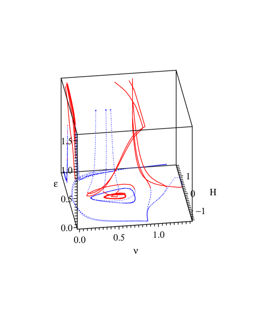
Figure 13: The trajectory of evolution in case of an interacting spinor and scalar fields with $\alpha=4,\beta=1,\zeta=1/2,A=1,B=1,m=4,\Lambda=-1,\lambda=-1$

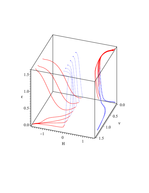
Figure 14: The trajectory of evolution in case of a spinor field with self-action at $\alpha=4,\beta=1,\zeta=1/2,A=1,B=1,m=4,\Lambda=-1,\lambda=-1$

In the figures 14 and 13 we show the evolution of $\tau$, $H$ and $\varepsilon$ relative to each other. In both cases there exists possibility for infinite growth of energy density at infinitely large volume, i.e., there occurs so-called Big Rip.

V Conclusion

Recently a self consistent system of nonlinear spinor and gravitational fields in the framework of Bianchi type-I cosmological model filled with viscous fluid was considered by one of the authors saharrp ; visnlsrev2 . The spinor filed nonlinearity is taken to be some power law of the invariants of bilinear spinor forms, namely $I=S^{2}=(\bar{\psi}\psi)^{2}$ and $J=P^{2}=(i\bar{\psi}\gamma^{5}\psi)^{2}$. Solutions to the corresponding equations are given in terms of the volume scale of the BI space-time, i.e., in terms of $\tau=abc$, with $a,b,c$ being the metric functions. This study generates a multi-parametric system of ordinary differential equations saharrp ; visnlsrev2 . Given the richness of the system of equations in this paper a qualitative analysis of the system in question has been thoroughly carried out. A complete qualitative classification of the mode of evolution of the universe given by the corresponding dynamic system has been illustrated. In doing so we have considered all possible values of problem parameters independent to their physical validity and graphically presented the most distinguishable in our view results.

The system is studied from the view point of blow up. It has been shown that in absence of viscosity the blow up does not occur. It should be emphasized that phenomena similar to one in question can be observed in other discipline of physics and present enormous interest from the point of catastrophe, demography etc.

References

(1) B. Saha and G.N. Shikin,
Journal of Mathematical Physics 38,
\htmladdnormallink5305http://wwwinfo.jinr.ru/ bijan/my_papers/JMP05305.pdf (1997).
(2) B. Saha, and G.N. Shikin, General
Relativity and Gravitation 29, \htmladdnormallink1099http://wwwinfo.jinr.ru/ bijan/my_papers/grg97_1099.pdf
(1997).
(3) Bijan Saha,
Physical Review D 64, \htmladdnormallink123501http://wwwinfo.jinr.ru/ bijan/my_papers/PRD23501.pdf (2001).
(4) Bijan Saha, Physics of Particles and Nuclei 37
Suppl. 1, \htmladdnormallinkS13-S44http://wwwinfo.jinr.ru/ bijan/my_papers/PHPS13.pdf, (2006).
(5) Bijan Saha, Physical Review D 74,
\htmladdnormallink124030http://wwwinfo.jinr.ru/ bijan/my_papers/PhysRevD_74_124030.pdf, (2006).
(6) Ribas, M.O., Devecchi, F.P., and Kremer, G.M.,
Phys. Rev. D 72 (2005) 123502.
(7) C.W. Misner, Astrophys. J. 151,
431 (1968).
(8) W. Misner, Nature 214, 40 (1967).
(9) S. Weinberg, Astrophysical Journal 168, 175 (1972).
(10) S. Weinberg, Gravitation and Cosmology
(New York, Wiley, 1972)
(11) P. Langacker, Physics report 72, 185 (1981).
(12) L. Waga, R.C. Falcan, and R. Chanda, Physical Review D
33, 1839 (1986).
(13) T. Pacher, J.A. Stein-Schabas, and M.S. Turner,
Physical Review D 36, 1603 (1987).
(14) Alan Guth, Physical Review D 23, 347 (1981).
(15) G.L. Murphy, Physical Review D 8, 4231 (1973).
(16) V.A. Belinski and I.M. Khalatnikov, Journal of Experimantal
and Theoretical Physics 69, 401, (1975).
(17) Bijan Saha, Modern Physics Letters A 20 (28)
\htmladdnormallink2127-2143http://wwwinfo.jinr.ru/ bijan/my_papers/mpla_05.pdf, (2005);
[arXiv: \htmladdnormallinkgr-qc/0409104http://xxx.lanl.gov/abs/gr-qc/0409104].
(18) Bijan Saha and V. Rikhvitsky, Physica D 219,
\htmladdnormallink168-176http://wwwinfo.jinr.ru/ bijan/my_papers/physD_06.pdf, (2006);
[arXiv: \htmladdnormallinkgr-qc/0410056http://xxx.lanl.gov/abs/gr-qc/0410056].
(19) Bijan Saha, Romanian Report of Physics 57
(1),\htmladdnormallink7-24http://wwwinfo.jinr.ru/ bijan/my_papers/romrep_05.pdf, (2005).
(20) Bijan Saha, Astrophysics and Space Science 312,
\htmladdnormallink3-11http://wwwinfo.jinr.ru/ bijan/my_papers/assvis07r.pdf, (2007)
[arXiv: \htmladdnormallinkgr-qc/0703085http://xxx.lanl.gov/abs/gr-qc/0703085].
(21) Bijan Saha and Victor Rikhvitsky,
Journal Physics A: Mathematical and Theoretical 40\htmladdnormallink14011-14027http://wwwinfo.jinr.ru/ bijan/my_papers/a7_46_013.pdf, (2007); \htmladdnormallinkarXiv:
0705.3128V1[gr-qc]http://xxx.itep.ru/PS_cache/arxiv/pdf/0705/0705.3128v1.pdf.
(22) Bijan Saha, Interacting spinor and scalar fields in Bianchi type-I Universe filled with viscous fluid: exact and numerical solutions
[arXiv: \htmladdnormallinkgr-qc/0703124http://xxx.lanl.gov/abs/gr-qc/0703124].
(23) A.A. Samarsky, V.A. Galaktionov, S.P. Kurdimov and A.P. Mikhailov, On unbound solutions of semi-linear parabolic equations
Preprint IPM. 1979. No 161.