The Knight field and the nuclear dipole-dipole field in an InGaAs/GaAs quantum dot ensemble

Abstract

We present a comprehensive investigation of the electron-nuclear system of negatively charged InGaAs/GaAs self-assembled quantum dots under the influence of weak external magnetic fields (up to 2 mT). We demonstrate that, in contrast to conventional semiconductor systems, these small fields have a profound influence on the electron spin dynamics, via the hyperfine interaction. Quantum dots, with their comparatively limited number of nuclei, present electron-nuclear behavior that is unique to low-dimensional systems. We show that the conventional Hanle effect used to measure electron spin relaxation times, for example, cannot be used in these systems when the spin lifetimes are long. An individual nucleus in the QD is subject to milli-Tesla effective fields, arising from the interaction with its nearest-neighbors and with the electronic Knight field. The alignment of each nucleus is influenced by application of external fields of the same magnitude. A polarized nuclear system, which may have an effective field strength of several Tesla, may easily be influenced by these milli-Tesla fields. This in turn has a dramatic effect on the electron spin dynamics, and we use this technique to gain a measure of both the dipole-dipole field and the maximum Knight field in our system, thus allowing us to estimate the maximum Overhauser field that may be generated at zero external magnetic field. We also show that one may fine-tune the angle which the Overhauser field makes with the optical axis.

I Introduction

The expectation that the electron spin in semiconductor quantum dots (QDs) could serve as a building block for quantum computing applications has drawn renewed attention to the role of the quantum dot nuclei. In the seventies it was shown that for bulk semiconductors, the interplay between an electron spin (at that time, of a donor trapped electron) and the nuclear spins in its vicinity leads to a wide variety of effects and often exhibits unexpected behavior lampel1968 ; ekimov1972 ; ekimovsafarov1972 ; berkovits1973 ; dyakonovperel1974 ; dyakonov1974 ; fleisher1975 ; paget1977 ; OptO . In QDs the hyperfine coupling between electron and nuclear spins is further enhanced by the strong localization of the electron in the dot, giving rise to complex dynamics merkulov2009 .

Nuclear spins can be polarized by transfer of angular momentum from optically oriented electrons, in a process known as the Overhauser effect overhauser1953 ; lampel1968 ; berkovits1978 . It was shown that nuclear polarization obtained in this way leads to an effective magnetic field of the order Tesla for the QD electron brown1996 ; gammon2001 ; koppens2005 ; akimov2006 ; eble2006 ; braun2006 ; tartakovskii2007 ; feng2007 ; maletinsky2007 ; oulton2007 . Most of these experiments exploited the Overhauser energy shift overhauser1953 ; brown1996 of the electron Zeeman levels split in an external field where the nuclear field was of the same order of magnitude as the external field.

In this paper we report experimental studies of InGaAs/GaAs quantum dots. We monitor the polarization of the QD ground state photoluminescence (PL) in the presence of weak external magnetic fields. The magnitude of these fields (a few mT or less) are shown to be far too small to have any direct effect on the dynamics of the electron in the QD itself. Milli-Tesla fields exerted onto electron spins only affect the spin precession dynamics over timescales greater than tens of nanoseconds. It is only recently that electron spin coherence times longer than this (several microseconds) have been observed in QDs greilich2006 . One might imagine that milli-Tesla magnetic fields may be used in this long coherence time regime to probe and manipulate spin dynamics, and in fact this has been reported epstein2001 ; bracker2005 . However, as we will demonstrate, considerable caution needs to be exercised in the interpretation of such data, as interactions are usually present which screen the direct effect of this external field on the electron.

For the above reasons, the influence of milli-Tesla fields onto the electron is usually negligible in semiconductors. It may come as a surprise, therefore, that we observe very dramatic effects on the electron polarization when applying these fields. This occurs in our system due to the fact that the electron dynamics are governed by the magnitude and direction of an effective nuclear, or Overhauser field that is exerted onto the electron from $\sim$10⁵ nuclei in the QD. By polarizing a significant fraction of these $\sim$10⁵ nuclear spins in the same direction, one may generate Tesla-strength Overhauser fields that completely dominate the electron spin dynamics in the system. The Tesla strength of these Overhauser fields is however deceptive: the interaction is not a real magnetic field, but an effective field that acts on the electron only.

While the sum of the interaction from all of the nuclear spins onto the electron is large, each nucleus itself is subject only to very small effective fields. Considered from the point of view of a single nucleus in the QD, the nucleus experiences three effective fields (i) from its nearest neighbors (the dipole-dipole field), of the order of magnitude of $\sim 0.1$ mT; (ii) from the electron, the Knight field, of the order of magnitude 0.1 – few mT; and (iii) any external fields applied. Thus in the regime of milli-Tesla applied fields, it is easy to see that we begin to explore the competition between the nearest neighbor field, the Knight field and the external field. We will demonstrate that by changing the magnitude and direction of external milli-Tesla magnetic fields, one may change the orientation of the Overhauser field. By first optically orienting the nuclear spins along the z-axis, and then applying a milli-Tesla magnetic field, one may induce a change in orientation of the entire Tesla-strength Overhauser field due to the precession of each nuclear spin about the external magnetic field.

The manuscript is divided into five sections. In Section II the samples and experimental technique are outlined. In Section III we describe how angular momentum is transferred from circularly polarized light to the electron-nuclear spin system in the QDs. In Section IV we consider theoretically the interaction between the electron and the nuclei in this system. Then in Section V the experimental results are discussed.

Section V.A explores what happens when a magnetic field is applied perpendicular to the optical axis. It is found that in this geometry, the applied field continuously reorients the nuclear spins away from the optical orientation direction, and thus build-up of a nuclear field is suppressed. This only occurs, however, when the applied field is larger than the nearest-neighbor interactions between the nuclei, and we use this technique therefore to measure the magnitude of the nearest-neighbor (dipole-dipole) interactions in our system.

In Section V.B we apply a field that is equal and opposite to the Knight field from the electrons, allowing us to obtain a value for this field. We refine the method used in previous work lai2006 by using a combination of fields perpendicular (transverse, $x$-direction) and parallel (longitudinal, $z$-direction) to the optical axis, allowing the Knight field feature to become more visible. In Section V.C we estimate theoretically the maximum degree of nuclear polarization we are able to obtain in our sample. Here we use the two important values we have measured, the Knight and dipole-dipole fields, the two quantities which govern spin diffusion in the system after the nuclear spins have been polarized. The Knight field acts to hold the polarization, whereas the dipole-dipole field allows spin diffusion. The ratio of these effective fields governs the nuclear polarization theoretically obtainable in our sample. We demonstrate that in principle, a nuclear polarization of up to $>$ 98 $\%$ may be generated.

II Samples and Experiment

The sample studied is a 20 layer InGaAs/GaAs self assembled QD ensemble with a sheet dot density of $10^{10}$ cm^-2. 20 nm below each QD layer a Silicon $\delta$-doping layer is located with a doping density about equal the dot density. Thus each QD is permanently occupied with on average one “resident electron”, as confirmed by pump-probe Faraday rotation measurements greilich2006 . The InAs/GaAs QD heterostructure was grown by molecular beam epitaxy on a (100) GaAs substrate. After growth it was thermally annealed for 30 seconds at 900℃. This leads to interdiffusion of Ga ions into the QDs, which shifts the ground state emission to 1.34 eV fafard1999 .

The measurements were performed at a temperature of $T=2$ K with the sample installed in an optical bath cryostat which was placed between three orthogonal pairs of Helmholtz coils allowing application of external magnetic fields of a few mT in all directions. The coils were used to compensate parasitic magnetic fields, of e. g. geomagnetic origin as well as to apply fields up to 3 mT parallel or perpendicular to the optical axis (longitudinal, $z$ direction or transverse, $x$ direction, respectively).

The optical excitation was performed using a mode locked Ti:Sapphire laser with a pulse duration of 1.5 ps and a repetition rate of 75.6 MHz (pulses separated by 13.2 ns). The excitation energy was 1.459 eV which corresponds to the low energy flank of the wetting layer. The helicity of the exciting light could be modulated by means of an electro-optical modulator and a $\lambda/4$ wave plate. With this setup pulse trains with duration between 20 $\mu s$ and 500 ms of $\sigma^{+}$ or $\sigma^{-}$ polarization were formed.

The beam was focused on the sample with a 10 cm focal length lens which was simultaneously used to collect the PL. The photoluminescence was dispersed with a 0.5 m monochromator and detected circular polarization resolved with a silicon avalanche photo-diode which was read out using a gated two-channel photon counter. In order to ensure a homogeneous excitation of the QDs the PL was collected from the center of the laser spot.

III Optical Orientation of electrons and negative circular polarization

The QDs studied contain on average one “resident” electron. After excitation of an electron-hole pair into the wetting layer and subsequent capture of the carriers into the QD, a trion is formed in these singly charged QDs. The trion ground state consists of two electrons in the conduction band s-shell with antiparallel spins and a single hole in the valence band s-shell. The helicity of the light emitted after the trion decays is therefore governed by the spin orientation of the hole. As a consequence, the helicity of the photon emitted directly determines the spin orientation of the resident electron left in the QD after radiative recombination.

It is an established phenomenon for singly n-doped QDs under non-resonant excitation and at zero magnetic field that the circular polarization degree $\rho_{c}$ of the emission has the opposite helicity to the excitation (known as negative circular polarization effect, NCP). Here we use the standard definition:

$$\rho_{c}=(I^{++}-I^{+-})/(I^{++}+I^{+-}),$$ (1)

with $I^{++}$ denoting the intensity of PL having the same helicity as the excitation ($\sigma^{+}$) and $I^{+-}$ the intensity of PL polarized oppositely to the excitation.

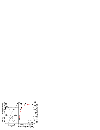
Figure 1: (a) (color online) PL spectra of the QD sample studied (lower panel). Excitation was $\sigma^{+}$ at 1.459 eV. The PL intensity of $\sigma^{-}$ emission is greater than that of $\sigma^{+}$ emission, thus the circular polarization degree is negative (upper panel). (b) Power dependence of the circular polarization degree $\rho_{c}$. $\rho_{c}$ rises with power and finally saturates indicating that a memory of the spin orientation of the resident electrons is kept until the following excitation cycle (see text). $P_{0}=2.5$ W/cm².

Figure 1 (a) depicts PL spectra of the QD ensemble studied under $\sigma^{+}$ excitation in the wetting layer, with detection either co-polarized ($\sigma^{+}$) or cross-polarized ($\sigma^{-}$) to the excitation. Both PL spectra show two peaks corresponding to the inhomogeneously broadened ground state emission at $\sim 1.34$ eV (s-shell), and to the first excited state emission at $\sim 1.37$ eV (p-shell). The polarization of the PL is negative throughout the emission from the s-shell (Fig. 1 (a), upper panel).

Different mechanisms explaining the NCP effect have been suggested cortez2002 ; kalevich2005 ; ware2005 ; verbin2005 ; akimov2005 ; laurent2006 ; masumoto2006 . In Ref. laurent2006 a mechanism was proposed whereby the anisotropic exchange between an excited state electron and the hole induces a spin exchange or “flip-flop” process, in order to overcome Pauli blocking of the ground state electrons with parallel spins. In Ref. ware2005 , it was suggested that dark excitons are preferentially captured from the wetting layer by the QDs. We note, however, that all of these mechanisms imply that the electron remaining after trion recombination accumulates spin polarization. This is the important feature we exploit in our experiments. The mechanism leading to this accumulation of electron spin polarization may still be subject to discussions, but is not decisive for our studies.

As in our previous work oulton2007 , we make use of this fact. We excite the system with 75.6 MHz pulsed circularly polarized excitation, allowing pumping of the electron spin population to occur. The electron spin polarization level reached in the sample is governed by the competition between the optical pumping rate and the decay dynamics of the electron spins. During our measurements, we always choose an excitation intensity well into the saturation regime. This ensures that when measuring the change in electron spin polarization, the effects we observe are due to changes in the decay rate of the electron spins, and not the optical pumping rate.

Figure 1 (b) shows the PL polarization as a function of excitation density. As expected, $\rho_{c}$ is strongly excitation power dependent. This dependence reflects the efficiency of the optical excitation of the dots, i. e. the average time between two excitation events. As the excitation power is increased, the electron spins become more polarized and $\rho_{c}$ increases until it reaches the saturation value of -27 to -30 %. The negative circular polarization is limited by the fraction of loaded QDs in the ensemble and the spin memory of the photoexcited electrons upon relaxation. Neutral excitons and biexcitons may also be created in the ensemble and spin preservation during relaxation from the wetting layer may not be perfect. Both these facts will reduce the $\rho_{c}$ value. Therefore, even with full resident electron spin polarization, the value of $\rho_{c}$ will not reach -100 %. In the NCP effect, both the photoexcited electrons that retain their polarization, and the polarized resident electron contribute to the negative polarization. One may estimate the circular polarization $\rho_{c}$ in a simple model: $\rho_{c}=Fx[P+S_{z}(I)]$, where $P$ is the average polarization of the photoinjected electron spins, independent of excitation intensity and $S_{z}(I)$ is the average polarization of the resident electron spin along the z-axis, and is dependent on excitation power. $F$ is the fraction of QDs in the sample that are singly charged and $x$ is the fraction of negatively circularly polarized photons emitted when either the photoexcited or the resident electron is polarized. Depending on the position on the sample, $F$ may be as large as 0.5 so that the electron spin polarization in the singly charged dots may actually be considerably larger, as the NCP measured. Thus we see that there is a linear dependence between NCP and resident electron spin polarization where the polarization of the photogenerated electron spins merely adds an offset. This is not crucial in our case as we solely discuss changes in NCP and thus electron spin polarization, respectively.

IV Orientation of nuclear spins and the electron-nuclear spin system

IV.1 Electron spin precession in the Overhauser field

In this section, we discuss in general terms the interaction between an electron in a QD and its constituent nuclei at $B_{ext}=0$. Recent theoretical khaetskii2000 ; merkulov2002 ; imamoglu2003 ; stepanenko2006 ; deng2006 and experimental dzhioev1999 ; braun2005 ; akimov2006 ; maletinsky2007 ; greilich2007 work has demonstrated that this is the key electron spin relaxation mechanism in QDs. In addition, strong Overhauser fields in QDs have been directly measured brown1996 ; tartakovskii2007 and inferred oulton2007 . We consider first of all the hyperfine interaction in QDs, and consider the effect of an Overhauser field onto the electron spin system under different optical orientation regimes. We then discuss the factors which influence the magnitude of the Overhauser field, before discussing the experimental results in milli-Tesla fields.

As an electron inside a QD is strongly localized, the interaction between electron spin and a nuclear spin is enhanced in comparison to bulk semiconductors. A single electron populating the conduction band of a QD has a Bloch wavefunction with s-symmetry, leading to a high electron density at the nuclear site. The envelope wavefunction has an overlap with about $10^{5}$ QD nuclei. This can be estimated by considering an approximately disk shaped QD 20 nm in diameter and 5 nm in height. Their spins interact with the electron spin via the hyperfine interaction, described by the Fermi contact Hamiltonian abragam1983

$$\hat{H}_{hf}=\sum_{i}A_{i}|\psi(\mathbf{R}_{i})|^{2}\,\hat{\mathbf{S}}\cdot\hat{\mathbf{I}}_{i}.$$ (2)

Here $|\psi(\mathbf{R}_{i})|^{2}$ is the probability density of the electron at the location $\mathbf{R}_{i}$ of the $i^{th}$ nucleus, $A_{i}$ is the hyperfine interaction constant and $\hat{\mathbf{S}}$, $\hat{\mathbf{I}}_{i}$ the operators of the electron spin and the nuclear spin, respectively.

As we see from Eq. (2), the total interaction energy is dependent on the electron spin, $\mathbf{S}$, and the orientation of each of the nuclear spins, $\mathbf{I}_{i}$. The interaction energy therefore crucially depends on the alignment of the nuclear spins in the QD. One may consider that the nuclei exert an effective magnetic field $\mathbf{B}_{N}$ onto the electron as given by

$$\left(\sum_{i}A_{i}|\psi(\mathbf{R}_{i})|^{2}\mathbf{I}_{i}\right)\cdot\mathbf{S}=g_{e}\mu_{B}\mathbf{B}_{N}\!\cdot\!{\mathbf{S}}.$$ (3)

where $g_{e}$ is the electron g-factor, $\mu_{B}$ the Bohr magneton.

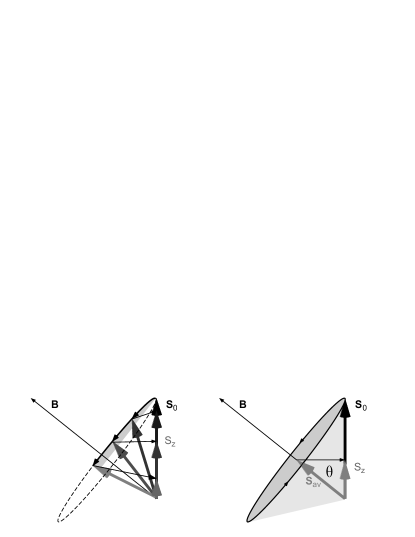
Figure 2: Schematic of electron spin precession in a nuclear field oriented at angle $\theta$ to the z-axis. The average electron spin vector is tilted at $\theta$. The polarization measured, however is given by the projection of this average electron spin onto the $z$-direction, such that $S_{z}=S_{0}\cos^{2}\theta$.

In light of the assumption that it is the hyperfine interaction that causes electron spin decay, we neglect other spin dephasing mechanisms (such as phonon interactions) at low temperatures and consider what happens to an electron spin in this nuclear magnetic field. The excitation pulse induces formation of a trion, which radiatively recombines to leave behind an electron spin polarized along the $\pm z$ direction (the optical axis). The electron spin dynamics are then governed by the effective field $\mathbf{B}_{N}$. In general, the motion of a spin $\mathbf{S}(t)$ in a fixed magnetic field $\mathbf{B}$ is described by

$$\mathbf{S}(t) = (\mathbf{S}_{0}\mathbf{\cdot b})\mathbf{b}+\left[\mathbf{S}_{0}-(\mathbf{S}_{0}\mathbf{\cdot b})\mathbf{b}\right]\cos\omega t+$$ (4)

$$\left[\left(\mathbf{S}_{0}-(\mathbf{S}_{0}\mathbf{\cdot b})\mathbf{b}\right)\times\mathbf{b}\right]\sin\omega t,$$

where $\mathbf{S}_{0}$ is the initial electron spin, $\mathbf{b}=\mathbf{B}/B$ is the unit vector in direction of the magnetic field acting on the electron and $\omega$ is the Larmor precession frequency given by $\omega=|g_{e}|\mu_{B}B/\hbar$. The dynamics of the electron spin at $B_{ext}=0$ is clearly dependent, therefore, on the direction of the Overhauser field, which may have any orientation in space. If the Overhauser field is aligned along the optical ($z$) axis, the electron spin will be static, and no polarization will be lost. For any $\mathbf{B}_{N}$ field not aligned along $z$, however, the electron spin evolves in time. In the classical analogue, the electron spin precesses about the $\mathbf{B}_{N}$ field.

In the measurements presented here, the electron spin precession period in $B\approx 25$ mT (the order of magnitude of the frozen nuclear spin fluctuation field, discussed below) is $\approx 5.7$ ns, compared to the 13 ns repetition period of the laser. The electron spin precesses more than twice before it is reinitialized. Here, we assume that the QD in which the electron is confined is excited by every pulse due to the high excitation intensity. By the time it is sampled by the next excitation pulse in PL, we measure a time average of this electron spin in the ensemble. If we average the $z$ component of $\mathbf{S}(t)$ over time we obtain

$$S_{z}(\mathbf{B})=S_{0}\frac{B_{z}^{2}}{B^{2}}\quad=S_{0}\cos^{2}(\theta(\mathbf{B})).$$ (5)

The expression for ${S}_{z}$ is obviously analogous to the z component of the projection of the initial electron spin $S_{0}$ on the precession axis defined by the magnetic field where $\theta$ is the angle between the precession axis and the $z$ axis (see Fig. 2).

Let us now consider what occurs in our system. Figure 2 shows the precession dynamics of the electron spin. The circularly polarized excitation results in spin population, giving an average initial electron spin $S(t=0)=S_{0}$. The electron precesses in the Overhauser field several times and the ensemble reaches a steady state of polarization $S_{0}\cos^{2}\theta$ before the next pulse arrives 13.2 ns later. This next pulse reads out the average projection of the electron onto the $z$-axis, as discussed in Section III. Thus the PL polarization is dependent on the initial electron spin $S_{0}$ and $\theta(\mathbf{B})$. $S_{0}$ is governed by the electron spin retained during energy relaxation from the wetting layer to the QD ground state. This is constant in our experiments, as the excitation conditions are kept the same. The angle of the Overhauser field to the $z$-axis, $\theta(\mathbf{B})$, is the factor that changes dramatically in these measurements, and we consider now what governs the magnitude and orientation of the Overhauser field.

IV.2 The nuclear magnetic field in the absence of optical orientation

In this Section we discuss the electron spin dynamics for the case where the nuclear spins are given no particular orientation. One might expect that in a system of randomly oriented nuclear spins, the nuclear magnetic field would be zero, and the electrons thus would be unaffected by the presence of the nuclei. Generally, however, the magnetic field generated by the sum of the nuclear spins is never exactly zero. The QD contains a large but nevertheless finite number of nuclei ($N=10^{5}$), which means that statistically, the number of spins parallel and antiparallel in any given direction will not be equal, but differ by a value $\sqrt{N/3}$ at a particular “snapshot” in time. The result is an effective magnetic field $B_{f}$, orientated in a random direction in 3D space, about which the electrons precess. The magnitude of $B_{f}$ can be estimated by $B_{f}=b_{N}/\sqrt{N}$ with $b_{N}$ being the maximum nuclear magnetic field for 100 % nuclear polarization. We estimate below a value of $b_{N}=8.3$ T for our QDs. For $N\approx 10^{5}$ one thus obtains $B_{f}\approx 26$ mT with an in-plane component of $B_{f,xy}\approx 20$ mT. Experimental values of 10 to 30 mT for $B_{f}$ agree well with this estimate ignatiev2007 .

How this $B_{f}$ field affects electron spin dephasing depends crucially on the timescale of reorientation of the nuclear spins compared to the precession period of the electron in $B_{f}$ (5 – 6 ns for $B_{f}\approx 25$ mT). Nuclear spin dynamics tend to be much slower than electron spin dynamics: the nuclear spin fluctuation field changes on a timescale of $10^{-6}$ s braun2005 ; comment1 due to the precession of the nuclear spins in the milli-Tesla magnetic field generated by the electron spin merkulov2002 (see Table 1 for an overview about the relevant timescales). This means that over timescales less than 1 $\mu$s, the electron is exposed to a ”snapshot” of $B_{f}$, where the nuclear spin configuration remains “frozen”. In the absence of an external magnetic field, only the internal field $\mathbf{B}=\mathbf{B}_{f}$ acts on the electron.

The direction and the magnitude of this frozen nuclear spin fluctuation will vary from dot to dot which leads to a rapid decay of the average electron spin orientation in the ensemble (note that this is also true for single dots when the electron polarization is measured as an average over many excitation cycles exceeding the nuclear fluctuation time). Despite the fact that the $B_{f}$ field is randomly oriented at any given time, the average electron spin measured over the ensemble does not decay to zero. Assuming that the nuclear spins are randomly distributed, $B_{f,x}=B_{f,y}=B_{f,z}$ and thus from Eq. (5):

$$\theta = \arccos{\frac{1}{\sqrt{3}}}\quad\widehat{=}\quad 54.7\degree,$$

$$S_{z} = \frac{S_{0}}{3}.$$ (6)

For a randomly oriented nuclear spin system, the average angle of $B_{f}$ is $\theta=54.7\degree$, and the electron spin polarization hence quickly decays to about 1/3 of its initial value due to the frozen nuclear field. Total decay then follows on a microsecond timescale due to continuous change in direction of this nuclear field merkulov2002 ; braun2005 . The value of 1/3 obviously arises from the fact that the projection onto all directions in 3D space is equal. The initial orientation of the electron is nevertheless important. In this system the electron starts with orientation along the $z$-axis but with no preferential direction in the $x$-$y$ plane, so that, when ensemble averaging, a residual projection onto the $z$-axis is retained, but no preferential direction exists in the $x$-$y$ plane.

IV.3 Optical orientation of the nuclear spins

Table 1: Typical timescales occuring in the electron-nuclear spin system assuming $g_{e}=0.5$ at zero external fieldmerkulov2002 ; OptO ; paget1977 .

precession of electron spin in $\sim 10$ mT $B_{f}$ field	$\sim 10^{-9}$ s
precession of nuclear spins in Knight field	$\sim 10^{-6}$ s
relaxation of nuclear spins in dipole-dipole field	$\sim 10^{-4}$ s
polarization of nuclear spins using NCP	$\sim 10^{-1}$ s

Strong optical pumping of the system with circularly polarized light leads to a continuous transfer of angular momentum from the photons to the electron spins. It is well-known that via spin flip-flops with polarized electrons, orientation of the nuclear spins along the axis of excitation may occur (Overhauser effect). For this process the respective orientation of the $B_{f}$ field in a QD at the point of time of the trion decay may be important. For QDs containing a $B_{f}$ field predominantly oriented along $z$ the electron spin’s $z$ projection stays large and thus enough time is given to flip a nuclear spin. However, in QDs where the $B_{f}$ field is by chance predominantly transverse, the electron spin precesses and is not able to polarize nuclear spins. While some $B_{f}$ configurations may inhibit electron spin preservation, the nuclear spin system changes on a microsecond timescale, so eventually most QDs will experience some nuclear polarization. Continuous optical pumping realigns the electron after angular momentum transfer to a nucleus, such that many nuclear spins become oriented. Without optical orientation, the nuclear fluctuation fields in every QD of the ensemble are evenly distributed in all three dimensions. With optical orientation, an additional field, the Overhauser field ${\bf B}_{N}$, is generated along the $z$ axis, that may be much larger than the in-plane component $B_{f,xy}$:

$$B_{N}>B_{f,xy}.$$ (7)

The electrons now precess about a nuclear field whose $z$ component dominates, resulting in an increase of average electron spin polarization $S_{z}$ in comparison to the case of a totally randomly oriented nuclear system. The angle $\theta$ in Eq. (5) decreases and $S_{z}$ increases.

A significant nuclear polarization obtained by strong pumping and sufficiently long illumination of the sample leads to a nuclear field $B_{N}\gg B_{f,xy}$ parallel to the $z$ axis and a marked reduction of the influence of the nuclear fluctuation field, maximally restoring electron spin alignment in $z$ direction ignatiev2007 . Note that at the very edges of the QDs nuclear spin diffusion out of the dot may occur, depending on the nuclear species. In the core of the QDs, however, where the Knight field is strong, spin diffusion is suppressed, and it is here that the nuclear spins may become polarized in our case.

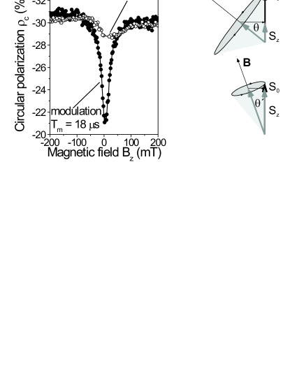
Figure 3: (a) Dependence of the negative circular PL polarization on a longitudinal magnetic field. For fast modulation of the excitation polarization (full circles) no significant nuclear polarization can build up and at $B_{z}=0$ the nuclear fluctuation field lead to depolarization of the ensemble average $S_{z}$. When $B_{z}$ becomes large enough to suppress the nuclear fluctuation field $B_{f}$ the polarization is maintained. Without modulation (open circles) nuclear polarization in $z$ direction builds up and the resultant $B_{N}$ field plays the same role as the external field, also at $B_{z}=0$. (b) Schematic for precession of the electron spin in the fluctuation field: (top) as in Fig. 2; and (bottom) for a total field at a shallower angle to the $z$-axis. For precession about the axis with $\theta^{\prime}<\theta$ more of $S_{z}$ is conserved.

Figure 3 (a) illustrates the effect of either an externally applied field or an internal field generated by nuclear polarization. Two curves are shown displaying the dependence of the PL polarization on an external field in $z$ direction. One of them was obtained for excitation helicity modulation between $\sigma^{+}$ and $\sigma^{-}$ with period $T_{m}=18\;\mu s$ which is about two orders of magnitude faster than the nuclear spins need to be polarized (with measurements performed during the $\sigma^{+}$ cycle only). The other one was recorded with unmodulated excitation, i. e. constant $\sigma^{+}$ excitation. Let us first consider the modulated excitation case. Here, the net angular momentum flux into the system averaged over time is zero and no significant nuclear polarization $B_{N}$ builds up (we will demonstrate in Sec. V.A that significant nuclear polarization requires tens of milliseconds pumping time). In this case, the $B_{f}$ field reduces the electron polarization at external field $B_{z}=0$ to about $-21$ %. When $B_{z}$ is increased, the resultant field $\mathbf{B}=\mathbf{B}_{z}+\mathbf{B}_{f}$ is at an angle closer to the $z$ axis ($\theta^{\prime}<\theta$). The projection of the electron polarization, given by Eq. (5), increases, and $\rho_{c}$ goes from $\approx-21$ % to $\approx-30$ %. For values $B_{z}\gg B_{f}$, $\theta^{\prime}\approx 0$ and the PL polarization saturates at $\approx-31$ %.

We now compare this to the case where a nuclear field is allowed to accumulate. Unmodulated excitation causes optical orientation of the nuclear spins even at $B_{z}=0$ and a nuclear field $B_{N}$ in $z$ direction builds up. This nuclear field plays exactly the same role as an external field in increasing the projection of the electron spin onto the $z$ axis. The resultant field onto the electron, given by $\mathbf{B}_{f}+\mathbf{B}_{N}$, is, again, closer to the $z$ axis. In this case, $B_{N}$ dominates over $B_{f}$. The polarization reaches $\approx-29$ % already at $B_{z}=0$, demonstrating that for almost all QDs, a significant nuclear polarization must occur. Note that the small dip which is still apparent for unmodulated excitation in Fig. 3 is caused by the ensemble distribution and the distribution of the $B_{f}$ field. While a large fraction of the QDs contains a polarized nuclear spin system there may still be some with less nuclear polarization. For higher external magnetic field, almost all of the of QDs house a strongly polarized nuclear spin system.

Note that in this work, the relative strength of the underlying fluctuation field, $B_{f}$, and the optically generated Overhauser field, $B_{N}$, hold the key to the electron spin dynamics. In fact, it is the presence of the significant fluctuation field as well as an optically generated Overhauser field that are unique to QDs in semiconductor systems.

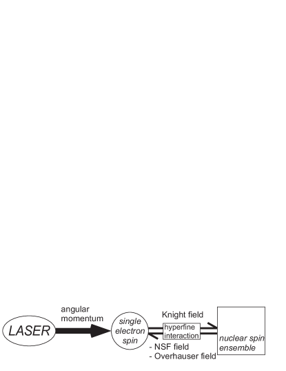
Figure 4: Summary of the interactions in the electron-nuclear spin system: A net angular momentum flux into the system is provided by the circularly polarized laser light. On a single spin level the electron and the nuclei interact via the hyperfine interaction. The action of the entirety of the nuclear spins upon the electron spin can be described by the Overhauser and the $B_{f}$ field. The nuclear spins of the ensemble relax due to the dipole-dipole interaction between them.

Figure 4 summarizes all the different influences between the resident electron spin, a single nuclear spin and the nuclear spin ensemble.

IV.4 The influence of Knight field and dipole-dipole interaction on nuclear spin polarization

We have discussed the effect of the nuclei on the electron spin until this point by considering them en masse. This approach is sufficient for explaining the optical orientation of the nuclear system as a whole, and the subsequent effect on the electron spin. The electron-nuclear system is, however, a highly interdependent coupled system, and to understand the electron spin dynamics one must also gain a detailed understanding of the nuclear spin dynamics. In this section, therefore, we consider what happens to a single nuclear spin as it interacts with its nearest neighbors, the electron and an external field.

The nuclear spin system is relatively isolated, such that in the absence of external magnetic fields, only two interactions dominate. First is the nearest-neighbor interaction. In an unpolarized nuclear ensemble, each nucleus experiences an effective magnetic field from the neighboring nuclear spins. This field (also known as the dipole-dipole field), denoted as $\tilde{B}_{L}$, is of the order of $0.1$ mT (as we experimentally confirm later) and fluctuates on the timescale of $10^{-4}$ seconds OptO . As we will see in the experimental results in Section V.A., the timescale for dynamic nuclear polarization is $10^{-2}$ seconds, two orders of magnitude slower than the dipole-dipole interaction. It has nevertheless been observed that even in zero applied external field conditions, significant nuclear polarization may occur in QDs oulton2006 ; lai2006 . The dipole-dipole interaction is not spin conserving, which leads to the question of why nuclear polarization may occur at all, and brings us onto the second interaction.

The second important interaction that a nuclear spin has with its environment is that with the electron (the hyperfine interaction). Equation 1 may be expanded to be expressed as:

$$\hat{H}_{hf}=\sum_{i}A_{i}|\psi(\mathbf{R}_{i})|^{2}\,[\hat{\mathbf{S}_{z}}\cdot\hat{\mathbf{I}}^{i}_{z}+(\hat{\mathbf{S}_{+}}\cdot\hat{\mathbf{I}}^{i}_{-}+\hat{\mathbf{S}_{-}}\cdot\hat{\mathbf{I}}^{i}_{+})/2].$$ (8)

The second term expresses the electron-nuclear spin flip-flop interaction responsible for the optical orientation of the nuclear spins, as described before. The first term, on the other hand, may be re-expressed as an effective magnetic field from the electron, $\mathbf{B}^{i}_{e}$, acting onto the $i^{th}$ nuclear spin:

$$\hat{H}_{hf}=-\hbar\mu_{i}\sum_{i}\hat{\mathbf{B}^{i}_{e}}\cdot\hat{\mathbf{I}}^{i}_{z}+\sum_{i}A_{i}|\psi(\mathbf{R}_{i})|^{2}(\hat{\mathbf{S}_{+}}\cdot\hat{\mathbf{I}}^{i}_{-}+\hat{\mathbf{S}_{-}}\cdot\hat{\mathbf{I}}^{i}_{+})/2,$$ (9)

where

$$\mathbf{B}^{i}_{e}=A_{i}|\psi(\mathbf{R}_{i})|^{2}\,\hat{\mathbf{S}_{z}}.$$ (10)

This effective field, the “Knight field”, was first identified in nuclear magnetic resonance (NMR) experiments knight1949 as a shift in frequency of the characteristic NMR resonance for particular metals. This shift occurs due to a paramagnetic effect from the presence of conduction band electrons, with the magnitude of this shift in energy being equal to the hyperfine splitting of the ground state of the atom. In our experiments, we cannot measure the Knight shift directly without NMR techniques, and so, as we will see in Section V, we apply a magnetic field equal and opposite to this Knight field and investigate the back-action effect on the Overhauser field.

From Eq. 10 we see that each nuclear spin experiences a Knight field that depends on (i) the location of the nucleus in the QD (the Knight field will be strongest for a nucleus in the centre of the QD, where $|\psi(\mathbf{R}_{i})|^{2}$ is largest) and (ii) $S_{z}$, the projection of the electron spin onto the $z$-axis. We have already discussed in Section IV.A that the electron precesses on a timescale of less than 10 ns, whereas the interaction of each nucleus is much slower than this. We may therefore use the time-averaged electron spin projection $S_{z}=S_{0}\cos^{2}\theta$, as given in Eq. 5.

In the absence of an external field, the value of the Knight field is an important quantity in determining whether nuclear polarization occurs. The effective field generated by the electron acts to screen the dipole-dipole interaction, and inhibits nuclear spin diffusion OptO ; lai2006 . If one makes the assumption that the maximum nuclear polarization may be achieved as long as dipole-dipole diffusion is completely suppressed, one may express the competition between the Knight field and the dipole-dipole field as OptO ; ThThesis :

$$\frac{B_{N}}{b_{N}} \approx \frac{B_{e}^{2}}{B_{e}^{2}+\tilde{B}_{L}^{2}}.$$ (11)

where $b_{N}$ is the maximum achievable nuclear field for a given alloy system. Thus, the value $B_{e}$ is an important one: a Knight field value significantly larger than the dipole-dipole field will allow nuclear polarization to occur. Due to Knight field variation, nuclear polarization will obviously vary across the QD.

Going back to Eq. 10 we see that the Knight field is also dependent on the electron spin polarization, $S_{z}$. We will see later that the experimentally determined value of the Knight field is dependent on the electron spin polarization, but it is also useful to define the maximum Knight field, $b^{i}_{e}$ for a given nucleus, such that:

$$\mathbf{B}^{i}_{e}=-b^{i}_{e}\frac{\langle\mathbf{S}\rangle}{S}.$$ (12)

where $b_{e}^{i}$ is the maximum Knight field at a particular nuclear site paget1977 ; OptO . The maximum Knight field is, in fact, the more important quantity to be determined in a particular QD system. As long as a strong nuclear field is generated ($B_{N}\gg B_{f}$) an electron will remain aligned along the $z$-axis, and the Knight field at all the nuclei will be the maximum possible in that system. As we will see later, in our experiments the only technique we have to probe the Knight field is to apply a field equal and opposite to it in order to depolarize the nuclei. At this point the average electron spin decreases significantly, and this must be taken into account when determining the experimental value of the Knight field value that we measure. However, although we measure $B_{e}$, we may extrapolate $b_{e}$ because we also have a value for $S_{z}$.

Finally, it is also important to note that in our experiment we determine a ”weighted average” value of the Knight field. The Knight field value will vary between each nucleus, going from a maximum value in the centre ($b^{max}_{e}$) to zero outside the QD. Making the approximation that $|\psi(r)|^{2}=\exp(-2r/a_{0})$, where $a_{0}$ is the radius of the QD and $r$ is the distance from the QD centre, one may estimate that the average value is equal to half the maximum Knight field $b^{max}_{e}/2$ foot1 . In Section V we will show that we measure a value of the Knight field, $\tilde{B}_{e}$, that is an average of the entire nuclear spin ensemble in the QD, and is also dependent on $S_{z}$.

V Results and Discussion

V.1 Hanle measurements and the dipole-dipole field

In this Section we discuss the application of a purely transverse magnetic field. We discuss the often-used interpretation of this type of experiment for determining the electron spin relaxation time, and demonstrate experimentally that for a QD system, this interpretation does not hold, and that in general it cannot be used for Hanle curve widths $<$ 10’s mT. We instead demonstrate that we may use this technique to determine the strength of nuclear dipole-dipole interactions in the system.

The Hanle effect hanle1924 is a technique often used in semiconductor physics to determine spin relaxation times by initializing spin in the system in a particular direction (e. g. along the $z$-axis) at time $t=0$ and monitoring the decrease of PL polarization as a transverse (known as Voigt geometry) magnetic field is applied OptO . An electron spin will precess in the $z$-$y$ plane, such that, according to Eq. (4), the dynamics will be given by $S_{z}(t)=S_{0}\cos(\omega t)$. When integrating over many cycles, the projection of the spin onto the $z$-axis is clearly zero for integration times considerably smaller than the spin lifetime. For a finite electron spin lifetime, $T_{S}$, however, the dynamics is given by $S_{z}(t)=S_{0}\exp(-t/T_{S})\cos(\omega t)$.

Figure 5: Dependence of the PL circular polarization degree on a transverse magnetic field $B_{x}$ under fixed circularly polarized excitation (full circles: measured data, solid line: Lorentz fit). When the external field is strong enough to overcome $\tilde{B}_{L}$ the nuclear spins precess about the external field leading to a reorientation of the Overhauser field along the external field. The electron spins become depolarized by precession about the nuclear field. In practice, however, for $B_{x}>\tilde{B}_{L}$ nuclear polarization is no longer generated and the electron spin is left with the fluctuation field (see text).

The Hanle effect hanle1924 may be used in a quantitative manner to determine the spin lifetime. The PL polarization is monitored as a Voigt geometry magnetic field is increased. Monitoring $S_{z}$ via the PL polarization whilst sweeping the transverse field yields a Lorentzian curve, the width of which is inversely proportional to the $T_{S}$ time of the electron:

$$T_{S}=\frac{\hbar}{|g_{e,x}|\mu_{0}B_{1/2}},$$ (13)

with the electron g factor $g_{e,x}$ along $x$, and the measured half width at half maximum $B_{1/2}$ of the Lorentz curve obtained.

Figure 5 shows a graph obtained from a Hanle measurement under unmodulated excitation, with pulses of 75.6 MHz repetition rate on our QD sample. A transverse magnetic field $B_{x}$ was swept and the PL polarization for each field value was recorded. The PL polarization drops sharply from its maximum value at $B_{x}=0$ the half-width of the peak being $\sim$ 0.22 mT. From the usual interpretation of the Hanle effect, Eq. (13), this would correspond to $T_{S}\sim 57$ ns assuming $g_{e,x}=0.5$ greilich2006 .

Let us now consider what happens if the excitation helicity is flipped between $\sigma^{+}$ and $\sigma^{-}$ with period $T_{m}$ that we are able to vary over a range of milliseconds. Fig. 6 shows Hanle curves under excitation modulated in such way (note that because the signal could only be measured during the $\sigma^{+}$ pulse, the measurement is inherently more noisy). The narrow peak appearing with unmodulated excitation at $B_{x}=0$ gradually disappears when the modulation frequency is increased. It almost completely vanishes for a modulation period of $T_{m}=1$ ms. This value is in complete disagreement with the value obtained from Eq. (13): if the electron spin relaxation time is of the order of $T_{2}^{\star}\sim 57$ ns, the slower 1 ms modulation should not inhibit it. In general, as the dynamics of the electron spin takes place on a nanosecond (precession) to microsecond (coherence) timescale (see Table 1), this millisecond effect is far too long to be of electronic origin. Although transverse fields also lead to the depolarization of polarized electron spins in the QDs under study, the situation obviously fundamentally differs from the one underlying the original Hanle effect.

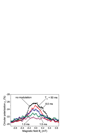
Figure 6: (color online) (a) Hanle curves for excitation modulated between $\sigma^{+}$ and $\sigma^{-}$ with period $T_{m}$ (smoothed). The narrow peak gradually vanishes for faster modulation and is almost absent for $T_{m}=1$ ms.

When considering the discussion in Section IV.B, it becomes immediately clear that the Hanle effect as discussed above should never be observed in this low field regime. In fact, it appears at first surprising that a dramatic change in the PL polarization is observed at all. As discussed in Section IV.B, the fluctuation field from the nuclei, $B_{f}\sim 10$’s mT, is always present and should screen completely the effect of any milli-Tesla applied field. Polarization of the nuclear spins may occur, but this will always result in an increase in the magnitude of the total nuclear magnetic field, $|\mathbf{B}_{f}+\mathbf{B}_{N}|$, which will always screen any mT applied field. Thus, care has to be taken when the width of the Hanle peak is used to determine the spin lifetime of the electron in QDs as has been suggested in the literature epstein2001 ; bracker2005 . This works only for nuclear fluctuation fields $B_{f}\ll 10$ mT. At fields lower than several tens of milli-Tesla the Overhauser field or the frozen fluctuation field will always dominate the spin dynamics in QDs.

The fact that an effect is only observed when tens of milliseconds excitation is used implies that the effect arises from dynamic nuclear polarization which is known to occur on these timescales gammon2001 ; maletinsky2007 . In the following we will explain the mechanisms leading to the specific shape of the curve in Fig. 6.

For modulated excitation with $T_{m}<1$ ms, almost no nuclear polarization is allowed to build up, and the electron feels the fluctuation field only. The electron spin decays to give $\rho_{c}\sim-21\%$ irrespective of the applied field. For unmodulated excitation on the other hand, a nuclear magnetic field builds up along the $z$ axis when $B_{x}=0$. The nuclear field adds to the frozen fluctuation field $B_{f,z}$ and reduces the angle $\theta$ between the $z$ axis and the total nuclear magnetic field $\mathbf{B}_{N,tot}=\mathbf{B}_{N}+\mathbf{B}_{f}$ as discussed in Sec. IV. The PL polarization, $\rho_{c}\propto S_{z}$ increases from $\sim-21$ % to $\sim-26$ % comment2 , similar to the behavior shown in Fig. 3.

Now let us consider what happens when a transverse field $B_{x}$ of a few mT is switched on. The electron is not sensitive to this field as it is screened by the much stronger nuclear fields (the fluctuation field or the Overhauser field), and so at first, it will continue to polarize the nuclear spins in the $z$-direction. The nuclear spins, however, are sensitive to this transverse field. As discussed in Section IV.D, the nuclei feel three fields: the external field $B_{x}$, the Knight field $B_{e}$ and the dipole-dipole field $\tilde{B}_{L}$, all of which are of the same order of magnitude. If the external field dominates over the other two, then over the timescale of $\mu$s, the nuclear spins begin to precess about this field.

This situation has been investigated in detail in Ref. paget1977 for donors in bulk GaAs. In this work, it was discussed that application of a magnetic field in an oblique direction results in the optically oriented nuclear spins precessing about this external field effectively aligning the Overhauser field along it. The electron still experiences this Overhauser field which is, however, now oriented along the external field: the Overhauser field effectively magnifies the external field by several orders of magnitude. This was described in reference paget1977 ; OptO as:

$$\mathbf{B}_{N}=\kappa(\mathbf{S},\mathbf{B}_{ext})\,\mathbf{B}_{ext},$$ (14)

where $\kappa$ is known as the multiplication factor. Note that the polarization of the nuclear spins only occurs due to optical orientation via the spin polarized resident electron, whereas the external field solely directs the optically generated Overhauser field. If an Overhauser field of several Tesla is generated and realigned to the external milli-Tesla magnetic field, $\kappa$ can reach values of $10^{3}$ or more. This extraordinary effect is the reason why such small external fields can have such a dramatic effect on the electron spin system.

For a purely transverse field, the polarized nuclear spins will precess about the $x$-direction in a few $\mu$s. This has the subsequent effect of destroying the electron spin polarization: it will precess about the $x$-axis and all projection onto the $z$-axis is lost. At this point, no further nuclear polarization via the electron spin can occur. The nuclear polarization already present will diffuse. Thus we see that dynamic nuclear polarization cannot occur in the steady state when a $B_{x}$ field is applied.

We observe though that a finite applied field is required to reduce the $\rho_{c}$. In Fig. 5 the PL value drops from $\sim$ -29$\%$ to $\sim$-24$\%$ steadily over the range of $\sim$0.6 mT and then does not decrease further. This fact may be explained by the presence of the dipole-dipole field $\tilde{B}_{L}$. For external magnetic fields $B_{x}<\tilde{B}_{L}$ the external field is screened by $\tilde{B}_{L}$. In order to realign the nuclear spins, $B_{x}$ has to dominate over the dipole-dipole field.

For measurements in a purely transverse magnetic field the $x$ component of the Knight field is zero, thus the only transverse field experienced by the nuclear spins is the external field. The width of the Hanle peak is hence solely determined by the competition between $\tilde{B}_{L}$ and $B_{ext}$. This is discussed further in OptO ; paget1977 . In this regime the width of the depolarization peak is a measure for the dipole-dipole field $\tilde{B}_{L}$ as discussed above. The average peak half width from several measurements corresponds to a dipole-dipole field of

$$\tilde{B}_{L}=0.22\pm 0.02\;\text{mT}.$$ (15)

We shall now examine what happens when $B_{x}$ is increased above the magnitude of $\tilde{B}_{L}$ and why the polarization remains at a constant level for $B_{x}\gtrsim$ 0.6 mT, and does not drop to zero, as may be expected if the field the electrons experience is purely transverse. To understand this behavior, one must consider the magnitude of the nuclear polarization field $B_{N}$ relative to the fluctuation field $B_{f}$. The field $B_{N}$ will decrease as $B_{x}$ increases: this is due to the fact that $B_{N}$ is dependent on $S_{z}$ and decreases with decreasing electron spin because then the ability of the electron spin to polarize the nuclear spins is reduced. Thus, at a sufficiently large $B_{x}$, the Overhauser field is close to zero, and only the fluctuation field $B_{f}$ remains. The fluctuation field then dominates the electron spin dynamics, and in Fig. 5 the $\rho_{c}$ value reaches $\approx$ -23 %, the value found at 0 T in Fig. 3 (a) for modulated excitation (i.e. with no nuclear polarization).

V.2 The Knight field

We have seen from Sec. V.A that the nuclei are sensitive to extremely small fields. In Section IV we also discussed the importance of the Knight field in allowing nuclear polarization. The Knight field $\tilde{B}_{e}$ is the effective magnetic field felt by each nucleus from the resident electron. $\tilde{B}_{e}$ is antiparallel to the electron spin, and in our scheme, is thus parallel to the $z$-axis. At $B_{ext}=0$ the Knight field screens the effect of the dipole-dipole field and allows dynamic nuclear polarization to occur; however, $\tilde{B}_{e}$ must be stronger than $\tilde{B}_{L}$ lai2006 ; paget1977 .

The magnitude of the Knight field is a quantity which varies not only between different QDs, but also between individual nuclei in a single QD, as its magnitude is proportional to the density of the electron wavefunction at a particular nuclear site. For QDs, the Knight field may be an order of magnitude stronger than in bulk, due to the increased electron density over fewer nuclei in the QD. This is why dynamic polarization in QDs at $B_{ext}=0$ can be much stronger than in bulk material. It is therefore of great interest to gain a measure of the strength of this effective field.

An approximate measure of the Knight field in QDs was determined for the first time by Lai et al. lai2006 . In this measurement, the PL polarization of a single QD exciton state was measured as a milli-Tesla field was swept along the $z$ direction. It was found that a dip in the polarization was visible at $\sim 0.6$ mT, whose position changed sign as the helicity of the excitation was changed. This decrease in polarization is due to the fact that the external field applied is exactly equal in magnitude and opposite in direction to the Knight field in that point, i. e. $B_{z}=-\tilde{B}_{e}$. A nucleus in the QD then experiences an approximate cancelation of the Knight field with the external field. Without the Knight field, dipole-dipole depolarization of the nuclear spins occurs quickly, and dynamic nuclear polarization does not build up.

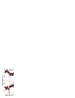
Figure 7: (color online) $B_{z}$ dependence of the PL polarization ($\rho_{c}$) for $B_{x}=0$ and fixed excitation polarization (full circles: measured data, solid line: smoothed). The dip at $B_{eff}=0$ is shifted from $B_{z}=0$ by the value of the Knight field $\tilde{B}_{e}$. Note that the sign of $\rho_{c}$ is opposite to the circular polarization of the excitation, see Eq. 1.

An identical measurement is performed in our system in the strong pumping regime, with the results shown in Fig. 7. Here, the $B_{z}$ dependence of the polarization is depicted for both excitation helicities. The PL polarization exhibits a barely discernible dip which is offset from $B_{z}=0$ and whose position is reversible with helicity. As in Ref. lai2006 , the shift corresponds to the external field which is needed to compensate the Knight field. However, the effect is very small. This is due to the fact that in an ensemble the Knight field is fairly inhomogeneous, and it is very difficult to depolarize all of the nuclear spins at the same time.

In our previous work oulton2007 we presented evidence that we achieve extremely large Overhauser fields ($>7$ T for some QDs) in our system. If this strong field is aligned along the $z$ axis, the polarization will be independent of the magnitude of $B_{N}$: as discussed in Section IV.C. As long as $B_{N}\gg B_{f}$ and aligned along the $z$-axis, the electrons do not depolarize. In order to see a visible effect when applying $B_{z}=-\tilde{B}_{e}$, one must reduce $B_{N}$ to be of the same order of magnitude as $B_{f}$. For an Overhauser field of a few Tesla, this means that $\sim 99\%$ of the nuclei contributing to this field must be depolarized simultaneously. We therefore use a method to measure the Knight field that was first reported in 1977 for electrons on donors paget1977 ; OptO , and present this method as ideal one for investigating the Knight field in QDs.

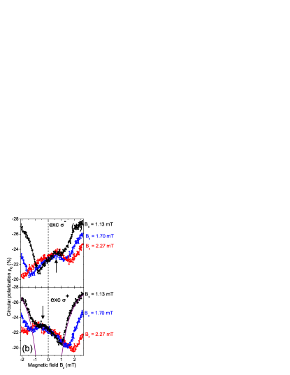
Figure 8: (color online) $B_{z}$ dependence of the PL polarization for different values of $B_{x}$: 1.13 mT, 1.7 mT and 2.27 mT. Excitation $\sigma^{-}$ (a) and $\sigma^{+}$ (b). The constant shift of the peak in the middle of the W-shaped structure (indicated by arrows) corresponds to the magnitude of the Knight field. Solid line in (b): Polarization behavior expected when the Knight field and the fluctuation field are neglected.

In order to make the Knight field more visible, we additionally apply a constant transverse magnetic field $B_{x}$, and again step the $B_{z}$ field. This technique, used extensively in paget1977 , allows one to access nuclear polarization regimes where $B_{N}$ is smaller, without significantly changing the electron spin polarization generated (as would be the case, for example, when decreasing the excitation power). In this technique, a transverse field is applied of magnitude 1.13 to 2.27 mT. The $z$-field is then swept, and the polarization is measured. By keeping the $B_{x}$ field constant and sweeping $B_{z}$, one effectively sweeps the angle, $\theta_{ext}$ that the total field $\mathbf{B}_{tot}=\mathbf{B}_{x}+\mathbf{B}_{z}$ makes with the $z$-axis, given by $\theta_{ext}=\arctan(B_{x}/B_{z})$. In fact, we will demonstrate that by using this technique, the angle that the $\mathbf{B}_{N}$ field makes with the $z$-axis may be finely tuned, and even become closer to the $x$-axis than $\theta=54\degree$, the angle at which the ensemble averaged frozen fluctuation field is generally tilted from the $z$ axis.

Let us consider what should be expected as the $B_{z}$ field is swept in the presence of a $B_{x}$ field. By sweeping the $B_{z}$ field, the angle of the total applied field is swept from $90\degree$ for $B_{z}=0$ to close to $0\degree$ when $B_{z}\gg B_{x}$. As in the rest of the work presented here, the applied field has no direct effect on the electron, but each of the nuclei will respond to this field, and in the absence of other effects, precess about the axis at an angle $\theta$.

Now let us assume that strong dynamic nuclear polarization is generated, where $B_{N}\gg B_{f}$. As we have discussed previously, the electron spin polarization is governed by this field: $S_{z}=S_{0}\cos^{2}\theta(B_{N})$. Thus sweeping the field should reveal a change in circular polarization from 0 to $-100\%$ if a strong $B_{N}$ field is created. In Fig. 8, $B_{z}$ dependencies for various applied transverse fields are shown for both $\sigma^{+}$ and $\sigma^{-}$ excitation. We do not observe the change from 0 to -100 %, despite the fact that clear changes in PL polarization occur on sweeping the field. A clear asymmetry is present, however, that is reversed upon reversal of the excitation polarization.

It is not surprising that the PL polarization does not drop to zero for low $B_{z}$ values. As in Fig. 5, for $\mathbf{S}_{0}\bot\mathbf{B}$, no nuclear polarization can occur. The electron spin, however, is still exposed to the nuclear fluctuation field which does not fully depolarize the electron spin. The value $\rho_{c}\sim$ -23 $\%$, is the same value as for $B_{x}\gg 0.22$ mT in Fig. 5, as we expect.

The solid line in Fig. 8 (b) shows the polarization behavior expected when the Knight field and the fluctuation field are neglected, and if we were to assume that $B_{N}$ is parallel to $B_{ext}$. The $B_{N}$ field direction would vary from $\theta=90\degree$ at $B_{z}=0$ T to $\theta=0\degree$ at $B_{z}\gg B_{x}$, and the time averaged electron spin $\langle\mathbf{S}\rangle$ would follow it also. In fact, as the $B_{N}$ field angle moves away from the $z$ axis, its magnitude decreases and the fluctuation field $B_{f}$ begins to dominate. For this reason the data do not follow the solid line.

The PL polarization exhibits a pronounced asymmetric W-shaped behavior on sweeping the longitudinal field, that is inverted on changing the excitation helicity. Let us consider first the points indicated by arrows in Fig. 8, corresponding to local turning points in the curve. These occur at $\sim\pm 0.5$ mT. We note that at these points, $\rho_{c}$ reaches a value of $\approx-23$ % for all the curves, and moreover, that these points, approximately correspond in magnitude and sign to the Knight field values observed in Fig. 7. At this point, the $B_{z}$ field approximately compensates the Knight field for many of the QD nuclei. Due to the cancelation of the Knight field the nuclear spins experience a purely transverse magnetic field. In this geometry nuclear polarization is not allowed to built up as $\mathbf{B}_{ext}\bot\mathbf{S}_{0}$. Thus the $\rho_{c}$ value measured corresponds to the fluctuation field value of $\approx-23$ %.

The marked asymmetry in the curves that are inverted when changing helicity allow easy determination of the compensation point, and this is indicated by the arrows in each figure. As soon as the $B_{z}$ field is swept away from the compensation point, nuclear polarization may begin to occur. Moving away from the compensation point, the magnitude of generated nuclear field $B_{N}$ increases. However, the magnitude of the $B_{N}$ field with respect to the fluctuation field $B_{f}$ and the orientation of $B_{N}$ has a complex effect on the resultant electron spin orientation, which we attempt to clarify in the next section.

V.3 Tuning the angle of the Overhauser field with milli-Tesla external fields

The experiment shown in Fig. 8 involves choosing an external $B_{x}$ field, which is kept constant, and sweeping another $B_{z}$ field, from negative to positive values, through zero. We therefore effectively sweep the angle of the external field from along the $x$-axis to along the $z$-axis, as explained previously. To further elucidate our data we have taken the same data shown in Fig. 8 (b) and replotted it, not as a function of $B_{z}$, but as a function of the angle of the total external field, as shown in Fig. 9. This angle is given by $\theta_{ext}=\arctan(B_{x}/B_{z})$. Note that $\theta_{ext}=90\degree$ and $0\degree$ corresponds to the external field along the $x$ and $z$ axes, respectively.

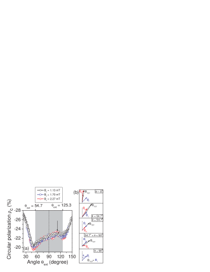
Figure 9: (a) Data from Fig.8 (b) replotted as a function of angle of applied field, $\theta_{ext}=\arctan(B_{x}/B_{z})$. Arrow shows approximate position of the Knight field compensation point. (b) series of schematics showing the magnitude and direction of the relevant nuclear fields for important regions of the applied field angle. Blue arrow: fluctuation field, $\mathbf{B}_{f}$; Red arrow: optically generated Overhauser field $\mathbf{B}_{N}$; Black arrow: resultant total nuclear field $\mathbf{B}_{tot}=\mathbf{B}_{f}+\mathbf{B}_{N}$

Upon replotting the data, it is evident that $\rho_{c}$ is dependent on $\theta_{ext}$ and not on the absolute magnitudes of $B_{x}$ or $B_{z}$. The curves for $B_{x}=$ 1.13, 1.70 and 2.27 mT obviously coincide, and show the same asymmetry as well as the W-shaped feature. The value of $\rho_{c}$ at the Knight field compensation point is $\sim$ -23 % (indicated by the arrows). Moving away from this point a reduction in $\rho_{c}$ is observed, until a turning point is reached, and $\rho_{c}$ then increases sharply. We now explain this behavior qualitatively.

In this experiment, the magnitude of the Overhauser field $B_{N}$ generated, is small, unless the applied $B_{z}$ field is very large. Therefore we are always in the regime where the Overhauser field generated is of the same order of magnitude as the fluctuation field ($B_{N}\sim B_{f}$), and the two are in direct competition. At the Knight field compensation point, the magnitude of $B_{N}$ is at its lowest, and the electron sees a pure $B_{f}$ field. The electron precesses around this fluctuation field, at $\theta_{f}=54.7\degree$ (first panel from bottom in Fig 9(b)).

Now let us consider what happens as we move away from $\theta_{ext}=90\degree$ towards the value 54.7$\degree$. We see that the polarization decreases, indicating that electron spin projection onto $z$ decreases. This appears counterintuitive. If the Overhauser field angle $\theta(\mathbf{B}_{N})$ of the polarized nuclear field is becoming closer to the $z$-axis, the electron polarization should increase. The second panel reveals why $S_{z}$ decreases in this region. The nuclear field generated for $\theta_{ext}>54.7\degree$ is much smaller in magnitude than $B_{f}$, but as $\theta_{ext}$ is decreased, the magnitude of $\mathbf{B}_{N}$ increases (due to the fact that $S_{z}$ is larger) and begins to compete more strongly with $\mathbf{B}_{f}$. It is clear from the second panel in Fig. 9(b) that for $\theta_{ext}>54.7\degree$, the total field $\mathbf{B}_{tot}=\mathbf{B}_{f}+\mathbf{B}_{N}$ is at a larger angle than $B_{f}$. This means that the stronger the Overhauser field $\mathbf{B}_{N}$ generated, the more the electron depolarizes.

At $\theta=54.7\degree$ a turning point is reached. At this point, $\mathbf{B}_{f}$ and $\mathbf{B}_{N}$ are at the same angle (see the third panel of Fig. 9(b)), and increasing $B_{N}$ is no longer detrimental. Upon increasing $\theta_{ext}$ further, any increase in $\mathbf{B}_{N}$ leads to a total field $\mathbf{B}_{tot}$ which is always at an angle smaller than $54.7\degree$. This has a positive feedback effect: the electron spin is preserved, and therefore may polarize more nuclei. As $\theta_{ext}$ is decreased further, $B_{N}$, and hence $S_{z}$ increase quickly, as depicted in the final panel at the top.

We have described the behavior shown in Fig. 8 in a quantitative way only. A qualitative description would require detailed knowledge of $\mathbf{B}_{N}$ as a function of angle, a value which is likely to be non-linear, and is beyond the scope of this paper. However, it shows clear evidence that these small external fields may be used to accurately fine-tune the angle of the Overhauser field generated. With improvements in nuclear pumping rate one may be able to control this angle over even wider ranges. The Overhauser field may therefore replace a strong external field used to manipulate electron spins, ranging from the Voigt to the Faraday geometry.

V.4 Evaluation of Knight field and nuclear field

Finally, in order to evaluate the Knight field we determine in Fig. 8 the magnetic field at which the Knight field was compensated. This compensation point has a position of

$$|\tilde{\mathbf{B}}_{e}|=0.5\pm 0.1\;\text{mT}.$$ (16)

This agrees well with the value of 0.6 mT which was measured in single QD experiments lai2006 .

From Eq. (12) in Section IV.D, it was discussed that each $i^{th}$ nucleus in the QD has an unique Knight field, $b^{i}_{e}$. In this experiment, a weighted average Knight field is measured: as discussed in Section IV.D, one may approximate this weighted average to be $\tilde{B}_{e}\sim B_{e,max}/2$ foot1 . The weighted average will clearly depend on the details of the electron confinement within the QD, which goes beyond the scope of this paper, but is not thought to deviate much from this approximation. We recall also that the measured Knight field will be reduced compared to the maximum obtainable Knight field, due to the fact that the average electron spin projection $S_{z}$ is reduced. Similarly to Eq. (12)

$$\mathbf{\tilde{B}}_{e}=-{\tilde{b}}_{e}\frac{\langle\mathbf{S}\rangle}{S}.$$ (17)

Let us now consider the compensation points $\tilde{\mathbf{B}}_{e}=-\mathbf{B}_{z}$ carefully again (arrows in Fig 8). At this point, the external field and internal Knight fields cancel, and generation of nuclear polarization is suppressed. The only field from the nuclei is now the fluctuation field $B_{f}$. As discussed before, the electron precesses about this field at $\theta=54.7\degree$, and thus, from Eq. (6), $S_{z}=S_{0}/3$. From Eq. (17), $\tilde{B}_{e}=\tilde{b}_{e}S_{z}/S_{0}$, it follows that:

$$\tilde{b}_{e}\sim 1.5\pm 0.3~{}\text{mT}.$$ (18)

The value $\tilde{b}_{e}$ gives the maximum Knight field onto the system if no depolarization of the electron spin occurs.

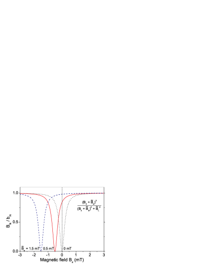
Figure 10: $(B_{z}+\tilde{B}_{e})^{2}/((B_{z}+\tilde{B}_{e})^{2}+\tilde{B}_{L}^{2})$ which is a measure for the competition between $\tilde{B}_{L}$ and $B_{e}$ concerning the ability of an Overhauser field to be generated. Values $\tilde{B}_{e}=0$, 0.5 and 1.5 mT are shown. The most important point to consider is the value at exactly $B_{z}=0$ (vertical dashed line), where no external field supports nuclear polarization.

The information we have gained about the magnitude of the Knight field and the dipole-dipole field now enable us to estimate the magnitude of the maximum achievable nuclear magnetic field using Eq. (11). In the calculations a leakage factor $f$ accounting for phenomenological losses of nuclear spin polarization not explicitly discussed here, was set to one so that the results should be understood as the maximum polarization which may be generated with the measured values $\tilde{B}_{e}=0.5$ mT and $\tilde{B}_{L}=0.22$ mT. Simply taking these values, one obtains a value for the estimated maximum field of:

$$\frac{B_{N}}{b_{N}} \approx \frac{\tilde{B}_{e}^{2}}{\tilde{B}_{e}^{2}+\tilde{B}_{L}^{2}}=0.84.$$ (19)

Thus we observe that even a moderate Knight field effectively dominates over the dipole-dipole field, and up to $84\%$ nuclear polarization may be obtained in the absence of any other leakage.

One may calculate $b_{N}$ in the case that $100\%$ of the nuclear spins are polarized. For In_0.5Ga_0.5As QDs with electron g-factor $g_{e}=0.5$ greilich2006 it was estimated that gueron1964 ; paget1977 ; oulton2007

$$b_{N,In_{0.5}} \approx -4.3\;T,$$

$$b_{N,Ga_{0.5}} \approx -1.26\;T,$$

$$b_{N,As} \approx -2.76\;T.$$ (20)

With these values we obtain a maximum nuclear field of $b_{N,max}=\sum_{i}b_{N,i}=-8.3$ T. This value is, in fact, exact for the alloy composition given and is independent of electron localization. From Eq. (19) therefore, we might expect to see an Overhauser field of $B_{N}=6.9$ T.

However, one should consider more carefully the value taken for the Knight field. In a system where little nuclear polarization has yet built up, the electron precesses around the $B_{f}$ field and, as we have shown, the residual electron spin polarization along $z$ gives rise to a Knight field of $\sim 0.5$ mT. It was in this regime that the Knight field was directly measured here. However, should a moderate Overhauser field build up in the $z$-direction that dominates over the fluctuating field, the electron does not precess about an oblique field, and both the electron spin projection and the Knight field reach their maximum values. We have already shown this maximum value to be $\tilde{b}_{e}\sim 1.5$ mT in this system. If we make the assumption that at $B_{ext}=0$ at least a moderate Overhauser field builds up in many of our QDs, we may use the maximum value of the Knight field ($B_{e}=b_{e}$)calculated from Eq. (18) to be

$$\frac{B_{N}}{b_{N}} \approx \frac{\tilde{b}_{e}^{2}}{\tilde{b}_{e}^{2}+\tilde{B}_{L}^{2}}=0.98.$$ (21)

Thus, we observe that as soon as a significant Overhauser field builds up in the QDs, the Knight field magnitude is at a maximum, and one should theoretically be able to obtain almost 100 % nuclear spin alignment (and an Overhauser field of $B_{N}=8.1$ T).

Note that the maximum projection of the Knight field onto the nuclei is not necessarily reflected in the measured $\rho_{c}$ value. The $\rho_{c}$ value is also governed by the probability of electron spin-flip from the wetting layer to the ground state during relaxation. Thus, the nuclear spins in a particular QD may be prepared with a strong alignment in the $z$ direction. An electron in the ground state therefore will not precess and lose its spin projection onto the $z$-axis. This is regardless of whether it has spin up or down. Thus while the sign of the Knight field will change if the electron is spin-flipped, the magnitude stays the same.

By way of illustration, Fig. 10. demonstrates the effect that different values of the Knight field have on the maximum obtainable nuclear polarization. In this figure, the function

$$\frac{B_{N}}{b_{N}} \approx \frac{(\mathbf{B}_{z}+\mathbf{\tilde{B}}_{e})^{2}}{(\mathbf{B}_{z}+\mathbf{\tilde{B}}_{e})^{2}+\tilde{B}_{L}^{2}}.$$ (22)

is plotted as a function of $B_{z}$ for Knight field values of $\tilde{B}_{e}=0,0.5,1.5$ mT, where $\tilde{B}_{L}$ is taken to be $0.22$ mT from Fig. 5. The vertical dashed line indicates the value $B_{z}=0$. It is clear here that for no Knight field, no nuclear polarization will occur according to this simple model, but for values of $\tilde{B}_{e}$ determined in this work, the nuclear polarization should reach large values.

In our previous work on the same sample oulton2007 strong evidence was found for high Overhauser fields, that allow the formation of a nuclear spin polaron state. The measurements here demonstrate that almost 100 % alignment should indeed be possible in these QDs. Note that we make the assumption that without dipole-dipole depolarization, 100 % alignment would be achieved. Clearly, the maximum nuclear polarization achievable is dependent on several factors, of which the Knight field magnitude is just one.

VI Summary and conclusions

We have demonstrated that the effect of negative circular polarization may be used both to polarize the spins of the resident electrons in n-doped QDs and to optically orient the nuclear spins in the QDs via spin transfer from the spin oriented electrons. Furthermore, the spin polarization of the resident electrons may be read out by measuring the circular polarization of the photoluminescence upon circularly polarized non-resonant excitation of the QDs.

The electron spin polarization at the same time serves as a sensitive detector for the state of the nuclear spin system. Milli-Tesla external magnetic fields may be used to manipulate the nuclear spins which in turn amplify the external field by orders of magnitude making it possible to detect their action via the electron polarization. Exploiting this co-dependence of electron and nuclear spins, we studied Hanle curves for excitation modulated between $\sigma^{+}$ and $\sigma^{-}$ helicity with different modulation periods. We were able to show that it takes tens of milliseconds to maximally polarize the nuclear spin system in the QDs using our polarization method. It became obvious that one has to examine thoroughly whether Hanle measurements in a specific case may be used to determine spin dephasing times of the electron. Even when nuclear polarization is suppressed by modulated excitation, the random frozen fluctuation nuclear field is still present, dominating the dynamics of the electron spins. Thus one may conclude that determining the electron spin lifetime using the Hanle effect for magnetic fields less than a few tens of milli-Tesla is incorrect due to screening either from the fluctuation field or the dynamic polarization: an alternative method must be used in QDs.

The Hanle measurements, however, allowed us to determine the dipole-dipole field $\tilde{B}_{L}\approx 0.22$ mT. Furthermore, the magnetic field dependence of the PL polarization in a combination of Faraday and Voigt geometries could be used to obtain an accurate determination of the magnitude of the Knight field $\tilde{b}_{e}\approx 1.5$ mT. It was also demonstrated that one may fine-tune the angle of $B_{N}$ to the $z$-axis.

After having determined the values of the dipole-dipole and Knight fields for this one system, the maximum nuclear field achievable may be calculated. It was found that, neglecting losses, the nuclear field at zero externally applied field may be as high as $\approx 6.9$ T, which is achievable due to the stabilizing influence of the Knight field. It was also calculated that the nuclear polarization could reach $>$ 98 % for a fully polarized electron spin, as the maximum Knight field value of $\approx$ 1.5 mT dominates over the dipole-dipole field. This nuclear field, reaching up to 8.1 T provides an explanation for the observation of polaron formation at $T=2$ K, as theoretically predicted merkulov1998 and for which some experimental evidence already has been provided oulton2006 ; oulton2007 .

The fact that we use a QD ensemble for our studies may be considered a disadvantage because of the ensemble inhomogeneities. However, the variation of the parameters of the electron-nuclear spin system we measure is not necessarily primarily due to the distribution in the ensemble but vary for a single QD due to the inhomogeneity over the dot volume. For a single QD, the nuclear configuration may be very different each time it is probed, and because the nuclear spins may remain frozen for microseconds to seconds, one must integrate over very long times to ensure true averaging effects. The fact that we do see collective effects in our sample is a proof that the ensemble broadening is relatively small concerning the parameters of the electron-nuclear spin system. On the contrary, it is a remarkable finding that the ensemble reacts collectively yielding the pronounced features we have observed.

To summarize, it is clear that the electron-nuclear system may be manipulated with just a few milli-Tesla, in stark contrast to conventional semiconductor systems. The dynamics of this complex system is only beginning to be understood, but clearly holds the key to achieving long electron spin qubit coherence times for use in applications such as quantum information processing, whilst the Knight field plays a crucial role in novel schemes for the use of QD nuclear spins as a quantum memorykurucz2009 .

References

- (1) e-mail: thomas.auer@e2.physik.uni-dortmund.de
-
(2)
Present address: Centre for Quantum Photonics, University of Bristol, Bristol BS8 1UB, United Kingdom.
e-mail: ruth.oulton@bristol.ac.uk - (3) Also in: A. F. Ioffe Physico-Technical Institute, Russian Academy of Sciences, 194021 St. Petersburg, Russia
- (4) G. Lampel, Phys. Rev. Lett. 20, 491 (1968).
- (5) A. W. Overhauser, Phys. Rev. 92, 411 (1953).
- (6) A. I. Ekimov and V. I. Safarov, ZhETF Pis. Red. 15, 453 (1972) [JETP Lett. 15, 319 (1972)].
- (7) V. L. Berkovits, A. I. Ekimov, and V. I. Safarov, Zh. Eksp. Teor. Fiz. 65, 346 (1973) [Sov. Phys. JETP 38, 169 (1974)].
- (8) M. I. D’yakonov, V. I. Perel’, V. L. Berkovits, and V. I. Safarov, Zh. Eksp. Teor. Fiz. 67, 1912 (1974) [Sov. Phys. JETP 40, 950 (1975)].
- (9) M. I. D’yakonov and V. I. Perel’, Zh. Eksp. Teor. Fiz. 65, 362 (1973) [Sov. Phys. JETP 38, 177 (1974)].
- (10) V. A. Novikov and V. G. Fleisher, Pis’ma Zh. Tekh. Fiz. 20, 935 (1975).
- (11) F. Meier and B. P. Zakharchenya (editors), Optical Orientation, Modern Problems in Condensed Matter Sciences, Vol. 8 (North-Holland, Amsterdam, 1984).
- (12) I. A. Merkulov, G. Alvarez, D. R. Yakovlev and T. C. Schulthess, arXiv:0907.2661 (2009).
- (13) D. Paget, G. Lampel, B. Sapoval, and V. I. Safarov, Phys. Rev. B 15, 5780 (1977).
- (14) A. I. Ekimov and V. I. Safarov, ZhETF Pis. Red. 15, 257 (1972) [JETP Lett. 15, 179 (1972)].
- (15) V. L. Berkovits, C. Hermann, G. Lampel, A. Nakamura, and V. I. Safarov, Phys. Rev. B 18, 1767 (1978).
- (16) S. W. Brown, T. A. Kennedy, D. Gammon, and E. S. Snow, Phys. Rev. B 54, R17339 (1996).
- (17) D. Gammon, Al. L. Efros, T.A. Kennedy, M. Rosen, D.S. Katzer, and D. Park, Phys. Rev. Lett. 86, 5176 (2001).
- (18) F.H.L. Koppens, J.A. Folk, J.M. Elzerman, R. Hanson, L.H. Willems van Beveren, I.T. Vink, H.P. Tranitz, W. Wegscheider, L.P. Kouwenhoven, and L.M.K. Vandersypen, Science 309, 1346 (2005)
- (19) I. A. Akimov, D. H. Feng, and F. Henneberger, Phys. Rev. Lett. 97, 056602 (2006).
- (20) B. Eble, O. Krebs, A. Lema tre, K. Kowalik, A. Kudelski, P. Voisin, B. Urbaszek, X. Marie, and T. Amand, Phys. Rev. B 74, 081306 (2006).
- (21) P.-F. Braun, B. Urbaszek, T. Amand, X. Marie, O. Krebs, B. Eble, A. Lemaitre, and P. Voisin, Phys. Rev. B 74, 245306 (2006).
- (22) A. I. Tartakovskii, T. Wright, A. Russell, V. I. Fal’ko, A. B. Van’kov, J. Skiba-Szymanska, I. Drouzas,1 R. S. Kolodka, M. S. Skolnick, P. W. Fry, A. Tahraoui, H.-Y. Liu, and M. Hopkinson, Phys. Rev. Lett. 98, 026806 (2007).
- (23) D. H. Feng, I. A. Akimov, and F. Henneberger, Phys. Rev. Lett. 99, 036604 (2007).
- (24) P. Maletinsky, A. Badolato, and A. Imamoglu, Phys. Rev. Lett. 99, 056804 (2007).
- (25) R. Oulton, A. Greilich, S. Yu. Verbin, R. V. Cherbunin, T. Auer, D. R. Yakovlev, M. Bayer, I. A. Merkulov, V. Stavarache, D. Reuter, and A. D. Wieck , Phys. Rev. Lett. 98, 107401 (2007).
- (26) A. Greilich, D. R. Yakovlev, A. Shabaev, Al. L. Efros, I.A. Yugova, R. Oulton, V. Stavarache, D. Reuter, A. Wieck, and M. Bayer, Science 313, 341 (2006).
- (27) R. J. Epstein, D. T. Fuchs, W. V. Schoenfeld, P. M. Petroff, and D. D. Awschalom, Appl. Phys. Lett. 78, 733 (2001).
- (28) A. S. Bracker, E. A. Stinaff, D. Gammon, M. E. Ware, J. G. Tischler, A. Shabaev, Al. L. Efros, D. Park, D. Gershoni, V. L. Korenev, and I. A. Merkulov, Phys. Rev. Lett. 94, 047402 (2005).
- (29) C. W. Lai, P. Maletinsky, A. Badolato, and A. Imamoglu, Phys. Rev. Lett. 96, 167403 (2006).
- (30) S. Fafard and C. Allen, Appl. Phys. Lett. 75, 2374 (1999).
- (31) S. Cortez, O. Krebs, S. Laurent, M. Senes, X. Marie, P. Voisin, R. Ferreira, G. Bastard, J-M. G rard, and T. Amand, Phys. Rev. Lett. 89, 207401 (2002).
- (32) S. Laurent, M. Senes, O. Krebs, V. K. Kalevich, B. Urbaszek, X. Marie, T. Amand, and P. Voisin, Phys. Rev. B 73, 235302 (2006).
- (33) M. Ikezawa, B. Pal, Y. Masumoto, I. V. Ignatiev, S. Yu. Verbin, and I. Ya. Gerlovin, Phys. Rev. B 72, 153302 (2005).
- (34) M. E. Ware, E. A. Stinaff, D. Gammon, M. F. Doty, A. S. Bracker, D. Gershoni, V. L. Korenev, S. C. Badescu, Y. Lyanda-Geller, and T. L. Reinecke, Phys. Rev. Lett. 95, 177403 (2005).
- (35) Y. Masumoto, S. Oguchi, B. Pal, and M. Ikezawa, Phys. Rev. B 74, 205332 (2006).
- (36) V. K. Kalevich, I. A. Merkulov, A. Yu. Shiryaev, K. V. Kavokin, M. Ikezawa, T. Okuno, P. N. Brunkov, A. E. Zhukov, V. M. Ustinov, and Y. Masumoto, Phys. Rev. B 72, 045325 (2005).
- (37) I. A. Akimov, K. V. Kavokin, A. Hundt, and F. Henneberger, Phys. Rev. B 71, 075326 (2005).
- (38) A. V. Khaetskii and Y. V. Nazarov Phys. Rev. B 61, 12639 (2000).
- (39) I. A. Merkulov, Al. L. Efros, and M. Rosen, Phys. Rev. B 65, 205309 (2002).
- (40) A. Imamoglu, E. Knill, L. Tian, and P. Zoller, Phys. Rev. Lett. 91, 017402 (2003).
- (41) D. Stepanenko, G. Burkard, G. Giedke, and A. Imamoglu, Phys. Rev. Lett. 96, 136401 (2006).
- (42) C. Deng, and X. Hu, Phys. Rev. B 73, 241303(R) (2006).
- (43) R. I. Dzhioev, B. P. Zakharchenya, V. L. Korenev, and M. V. Lazarev, Phys. Solid State 41, 2014 (1999).
- (44) P.-F. Braun, X. Marie, L. Lombez, B. Urbaszek, T. Amand, P. Renucci, V. K. Kalevich, K. V. Kavokin, O. Krebs, P. Voisin, and Y. Masumoto, Phys. Rev. Lett. 94, 116601 (2005).
- (45) A. Greilich, A. Shabaev, D.R. Yakovlev, Al. L. Efros, I.A. Yugova, D. Reuter, A.D. Wieck, and M. Bayer, Science 317, 1896 (2007).
- (46) A. Abragam, The Principles of Nuclear Magnetism, (Clarendon Press, Oxford, 1983)
- (47) R. V. Cherbunin, S. Yu. Verbin, T. Auer, D. R. Yakovlev, D. Reuter, A. D. Wieck, I. Ya. Gerlovin, I. V. Ignatiev, D. V. Vishnevsky and M. Bayer, Phys. Rev. 80, 035326 (2009).
- (48) R. Oulton, S. Yu. Verbin, T. Auer, R. V. Cherbunin, A. Greilich, D. R. Yakovlev, M. Bayer, D. Reuter, and A. Wieck, Phys. Stat. Sol. (b) 243, 3922 (2006).
- (49) W. D. Knight, Phys. Rev. 76, 1259 (1949).
- (50) T. Auer, PhD. Thesis: “The electron-nuclear spin system in (In,Ga)As quantum dots” (Sierke Verlag, Goettingen, 2008).
- (51) This weighted average reflects the fact that, while for a nucleus at a distance the Knight field value is , the contribution this nucleus makes to the Overhauser field is of that of a nucleus at the centre. Thus the average Knight field value measured is fairly narrow and weighted heavily towards the nuclei in the QD center.
- (52) W. Hanle, Z. Phys. 30, 93 (1924).
- (53) M. Gueron, Phys. Rev. 135, A200 (1964).
- (54) I. A. Merkulov, Phys. Solid State 40, 930 (1998).
- (55) The dominant mechanism for the evolution of the nuclear spins over this timescale is still under debate: both direct precession of the nuclear spins in the electronic field and electron mediated nuclear-nuclear spin-flip processes are thought to play a role. In any case, it is in fact the electron itself that causes nuclear spin evolution maletinsky2007 : without an electron present only the dipole-dipole interaction is important.
- (56) Note that the maximum and minimum values of vary slightly between Figs. 5 and 6, with the maximum varying from %. This is because the measurements are taken on different measurement runs. As we have demonstrated in reference oulton2007 , slight temperature variations in the bath cryostat give rise to different values of nuclear polarization decay over very long times. The behavior of the changes in polarization in this paper when a magnetic field is swept are not strongly dependent on temperature, however. Additionally, slight changes in excitation wavelength result in a change in electron spin memory preserved during energy relaxation from the wetting layer. Again, this slight variation does not affect the electron-nuclear spin dynamics here.
- (57) Z. Kurucz, M. W. Sorensen, J. M. Taylor, M. D. Lukin, M. Fleischhauer, Phys. Rev. Lett. 103, 010502 (2009).