Vortex solutions of the discrete Gross-Pitaevskii equation

Abstract

In this paper, we consider the dynamical evolution of dark vortex states in the two-dimensional defocusing discrete nonlinear Schrödinger model, a model of interest both to atomic physics and to nonlinear optics. We find that in a way reminiscent of their 1d analogs, i.e., of discrete dark solitons, the discrete defocusing vortices become unstable past a critical coupling strength and, in the infinite lattice, they apparently remain unstable up to the continuum limit where they are restabilized. In any finite lattice, stabilization windows of the structures may be observed. Systematic tools are offered for the continuation of the states both from the continuum and, especially, from the anti-continuum limit. Although the results are mainly geared towards the uniform case, we also consider the effect of harmonic trapping potentials.

, , , .

1 Introduction

The study of vortices and their existence, stability and dynamical properties has been a central theme of study in the area of Bose-Einstein condensates (BECs) [1, 2]. In particular, the remarkable experiments illustrating the generation of vortices [3, 4, 5] and of very robust lattices thereof [6, 7, 8] have stirred a tremendous amount of activity in this area in the past few years, that has by now been summarized in various reviews and books; see for example [9, 10, 11, 12, 13, 14]. Much of this activity has been centered around the robustness of vortex structures in the context of the mean-field dynamics of the BECs (which are controllably accurately described by a nonlinear Schrödinger (NLS) equation) in the presence of many of the potentials that are relevant to the trapping of atomic BECs including parabolic traps [1, 2] and periodic optical lattice ones [15, 16]. Particularly, the latter context of optical lattice potentials is quite interesting, as it has been suggested that vortices (for example of topological charge $S=1$) will be unstable when centered at a minimum of the lattice potential [17], an instability that it would be interesting to understand in more detail.

On the other hand, the BECs in the presence of periodic potentials have been argued to be well-approximated by models of the discrete nonlinear Schrödinger (DNLS) type (i.e., resembling the finite-difference discretization of the continuum equation) [18, 19, 20, 21]. In that regard, to understand the existence and stability properties of vortices in the presence of periodic potentials, it would be interesting to analyze the discrete analog of the relevant NLS equation. This is also interesting from a different perspective in this BEC context, namely that if finite-difference schemes are employed to analyze the properties of the continuum equation, it is useful to be aware of features introduced by virtue of the discretization.

However, it should be stressed that this is not a problem of restricted importance in the context of quantum fluids; it is also of particular interest in nonlinear optics where two-dimensional optical waveguide arrays have been recently systematically constructed e.g. in fused silica in the form of square lattices [22, 23] (and, more recently of even more complex hexagonal lattices [24]), whereby discrete solitons can be excited. By analogy to their one-dimensional counterparts of discrete dark solitons, which have been created in defocusing waveguide arrays with the photovoltaic nonlinearity [25], we expect that it should be possible to excite discrete dark vortices in defocusing two-dimensional waveguide arrays. An especially interesting feature of dark solitons that was observed initially in [26] (see also [27]) is that on-site discrete dark solitons are stable for sufficiently coarse lattices, but they become destabilized beyond a certain coupling strength among adjacent lattice sites and remain so until the continuum limit where they are again restabilized (as the point spectrum eigenvalue that contributes to the instability becomes zero due to the restoration of the translational invariance in the continuum problem) [26, 27]. It is therefore of interest to examine if the instability mechanisms of discrete defocusing vortices are of this same type or are potentially different and how the relevant stability picture is modified as a function of the inter-site coupling strength.

It is this problem of the existence, stability and continuation of the vortex structures as a function of coupling strength that we examine in the present work. We consider, in particular, a two-dimensional discrete non-linear Schrödinger equation

$$i\frac{d\psi_{n,m}}{dt}-|\psi_{n,m}|^{2}\psi_{n,m}+\epsilon\Delta\psi_{n,m}=0,$$ (1)

where $\Delta\psi_{n,m}=\psi_{n+1,m}+\psi_{n-1,m}+\psi_{n,m+1}+\psi_{n,m-1}-4\psi_{n,m}$ is the discrete Laplacian. We study the defocusing case when $\epsilon>0$. In that case, equation (1) is denoted as discrete Gross-Pitaevskii equation in analogy with its continuum counterpart [1, 2, 28].

We look for time-periodic solutions with frequency $\omega$. Using the ansatz $\psi_{n,m}(t)=\sqrt{\omega}\,\phi_{n,m}e^{-i\omega t}$, we obtain

$$C\,\Delta\phi_{n,m}+(1-|\phi_{n,m}|^{2})\phi_{n,m}=0,$$ (2)

where we have set $C=\epsilon/\omega$. The coupling parameter $C>0$ determines the strength of discreteness effects. The limit $C\rightarrow+\infty$ corresponds to the continuum (stationary) Gross-Pitaevskii equation:

$$\frac{\partial^{2}\phi}{\partial x^{2}}+\frac{\partial^{2}\phi}{\partial y^{2}}+(1-|\phi|^{2})\phi=0.$$ (3)

The case $C\rightarrow 0$ corresponds to the so-called anti-continuum (AC) limit [29].

When equation (2) is considered on an infinite lattice $\mathbb{Z}^{2}$, we look for solutions satisfying $|\phi_{n,m}|\rightarrow 1$ when $(n,m)\rightarrow\infty$, for which $\phi_{n,m}$ vanishes at one lattice site, e.g. at $(n,m)=(0,0)$. Such solutions are denoted as discrete vortices, or “dark” vortex solitons. If one trigonometric turn on any path $\mbox{Max}(|n|,|m|)=\rho$ around the vortex center changes the argument of $\phi_{n,m}$ by $2\pi S$ ($S\in\mathbb{Z}$), then the vortex is said to have a topological charge (or vorticity) equal to $S$.

In this paper we numerically investigate the existence and stability of such solutions on a finite lattice of size $N\times N$, $N$ being large; our analysis is performed as a function of the lattice coupling parameter $C$ and we illustrate how to perform relevant continuations both from the continuum, as well as, more importantly from the AC limit (section 2). We mainly focus on numerically computing vortex solutions with vorticity $S=1$ and $S=2$ (section 3). In section 4, we also obtain such solutions in the presence of an external harmonic trap (the latter is typically present in BEC experiments). Finally, section 5 presents our conclusions and some future directions of potential interest.

2 Numerical method

We compute vortex solutions of (2) using the Newton method and a continuation with respect to $C$. The path-following can be initiated either near the continuum limit (for $C$ large) or at the anti-continuum limit $C=0$, since in both cases one is able to construct a suitable initial guess for the Newton method.

For relatively high $C$, a suitable initial condition for a vortex with topological charge $S$ is obtained with a Padé approximation developed for the continuum limit in [28]. We set $\phi_{n,m}=\rho_{n,m}e^{iS\alpha_{n,m}}$, where

$$\rho_{n,m}=\sqrt{\frac{r_{n,m}^{2S}(a_{1}+a_{2}r_{n,m}^{2})}{1+b_{1}r_{n,m}^{2}+a_{2}r_{n,m}^{2S+2}}},\ \ \ \ r_{n,m}=\sqrt{n^{2}+m^{2}}$$ (4)

($a_{1}=11/32$, $a_{2}=a_{1}/12$, $b_{1}=1/3$, see reference [28]),

$$\alpha_{n,m}=\left\{\begin{array}[]{ll}\arctan(m/n)+\frac{3\pi}{2}&\mbox{ for }n\geq 1,\\ \arctan(m/n)+\frac{\pi}{2}&\mbox{ for }n\leq-1,\\ \frac{\pi}{2}\,(1-\mbox{sign}(m))&\mbox{ for }n=0.\end{array}\right.$$

Once a vortex is found for a given $C$, the solution can be continued by increasing or decreasing $C$. Although this method was found to be efficient, it remains limited to single vortex solutions having explicit continuum approximations. Moreover, when the Newton method is applied to continue these solutions near $C=0$, the Jacobian matrix becomes ill-conditioned (and non-invertible for $C=0$) and the iteration does not converge.

In what follows we introduce a different method having a wider applicability, and for which the above mentioned singularity is removed. We consider a finite $N\times N$ lattice with $(n,m)\in\Gamma=\{-M,\ldots,M\}^{2}$ ($N=2M+1$), equipped with fixed-end boundary conditions given below. We set $\phi_{n,m}=R_{n,m}\,e^{i\theta_{n,m}}$ and note $R=(R_{n,m})_{n,m}$, $\theta=(\theta_{n,m})_{n,m}$. One obtains the equivalent problem

$$R_{n,m}\,(1-R_{n,m}^{2})+C\,f(R,\theta)_{n,m}=0,$$ (5)

$$C\,g(R,\theta)_{n,m}=0,$$ (6)

where $f(R,\theta)=\mbox{Re }[\,e^{-i\theta}\,\Delta(R\,e^{i\theta})\,]$ and $g(R,\theta)=\mbox{Im }[\,e^{-i\theta}\,\Delta(R\,e^{i\theta})\,]$ can be rewritten

$$f(R,\theta)_{n,m} = R_{n+1,m}\cos{(\theta_{n+1,m}-\theta_{n,m})}+R_{n-1,m}\cos{(\theta_{n,m}-\theta_{n-1,m})}-4R_{n,m}$$

$$+R_{n,m+1}\cos{(\theta_{n,m+1}-\theta_{n,m})}+R_{n,m-1}\cos{(\theta_{n,m}-\theta_{n,m-1})},$$

$$g(R,\theta)_{n,m} = R_{n+1,m}\sin{(\theta_{n+1,m}-\theta_{n,m})}-R_{n-1,m}\sin{(\theta_{n,m}-\theta_{n-1,m})}$$

$$+R_{n,m+1}\sin{(\theta_{n,m+1}-\theta_{n,m})}-R_{n,m-1}\sin{(\theta_{n,m}-\theta_{n,m-1})}.$$

Now we divide equation (6) by $C$ (this eliminates the above-mentioned degeneracy at $C=0$) and consider equation (5) coupled to

$$g(R,\theta)_{n,m}=0.$$ (7)

System (5), (7) is supplemented by the boundary conditions

$$R_{n,m}=1 \mbox{Max}(|n|,|m|)=M,$$ for (8)

$$\theta_{n,m}=\theta_{n,m}^{\infty} \mbox{Max}(|n|,|m|)=M.$$ for (9)

The prescribed value $\theta_{n,m}^{\infty}$ of the angles on the boundary will depend on the type of vortex solution we look for. In particular, we use the boundary conditions $\theta_{n,m}^{\infty}=S\alpha_{n,m}$ for a single vortex with topological charge $S$ centered at $(n,m)=(0,0)$.

For $C=0$, a single vortex at $(n,m)=(0,0)$ corresponds to fixing $R_{0,0}=0$ and $R_{n,m}=1$ everywhere else. Equation (7) yields in that case

$$\begin{array}[]{l}\sin{(\theta_{n+1,m}-\theta_{n,m})}-\sin{(\theta_{n,m}-\theta_{n-1,m})}\\ +\sin{(\theta_{n,m+1}-\theta_{n,m})}-\sin{(\theta_{n,m}-\theta_{n,m-1})}=0,\\ (n,m)\in\Gamma\setminus\{\,(0,\pm 1),\,(\pm 1,0)\,,\,(\pm M,m)\,,\,(n,\pm M)\,\}\end{array}$$ (10)

supplemented by the four following relations at $(n,m)=(0,\pm 1),\,(\pm 1,0)$

$$\sin{(\theta_{1,\pm 1}-\theta_{0,\pm 1})}-\sin{(\theta_{0,\pm 1}-\theta_{-1,\pm 1})}+\sin{(\theta_{0,\pm 2}-\theta_{0,\pm 1})} = 0,$$ (11)

$$\sin{(\theta_{\pm 2,0}-\theta_{\pm 1,0})}+\sin{(\theta_{\pm 1,1}-\theta_{\pm 1,0})}-\sin{(\theta_{\pm 1,0}-\theta_{\pm 1,-1})} = 0.$$ (12)

For a vortex with topological charge $S=1$, solutions of (9)-(12) are computed by the Newton method, starting from the initial guess $\theta_{n,m}=\alpha_{n,m}$. The symmetries of the problem allow one to divide by four the size of the computational domain. Indeed one can take $(n,m)\in\{0,\ldots,M\}^{2}$ with the boundary conditions $\theta_{0,m}=\alpha_{0,m}$, $\theta_{n,0}=\alpha_{n,0}$. Solutions on the whole lattice $\Gamma$ have the symmetries

$$\theta_{n,-m}=\pi-\theta_{n,m}\,[2\pi],\ \ \ \ \theta_{-n,m}=-\theta_{n,m}\,[2\pi].$$ (13)

These conditions make (10) automatically satisfied at $(n,m)=(0,0)$ ($\theta_{0,0}$ need not being specified). Afterwards, the corresponding solution of (5), (7)-(9) can be continued to $C>0$ by the Newton method, yielding a solution $\phi_{n,m}=R_{n,m}e^{i\theta_{n,m}}$ of (2) (see section 3). For higher topological charges, the initial guess $\tilde{\phi}_{n,m}=R_{n,m}e^{iS\theta_{n,m}}$ can be used to compute a vortex solution of (2) by the Newton method. This is done in section 3 also for $S=2$. All these continuations are performed with a $10^{-8}$ accuracy.

3 Numerical computation of single vortices

In this section we analyze the existence and stability of discrete vortices centered on a single site, as a function of the coupling strength $C$ for fixed-end boundary conditions. The stability of the discrete vortex solitons is studied assuming small perturbations in the form of $\delta\psi_{m,n}=\exp(-it)[p_{n,m}\exp(-i\lambda t)+q_{n,m}\exp(i\lambda^{*}t)]$, the onset of instability indicated by the emergence of $\mathrm{Im}(\lambda)\neq 0$; $\lambda$ in this setting denotes the perturbation eigenfrequency. Note that it is sufficient to consider the case $\omega=1$ for stability computations, because this case can always be recovered by rescaling time.

Figure 1 compares the computed angles $\theta_{n,m}$ with respect to the seed angle $\alpha_{n,m}$ for fixed-end boundary conditions and $N=81$. The most significant differences arise close to the vortex center. This figure also shows the dependence on $N$ of the difference between the angles $\theta$ for a given domain size $N$ and for a larger domain of size $N+10$. This is done through $||\theta_{n,m}^{N}-\theta_{n,m}^{N+10}||$ where $||\cdot||$ is the $\infty$-norm, and $\theta_{n,m}^{N}$ represent the angles at a given lattice size $N$. The main contribution of this norm corresponds to the boundary sites. On the other hand, the decrease of this norm as a function of $N$ originates from the convergence of the configuration to an asymptotic form.

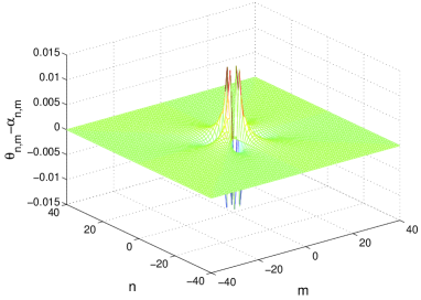
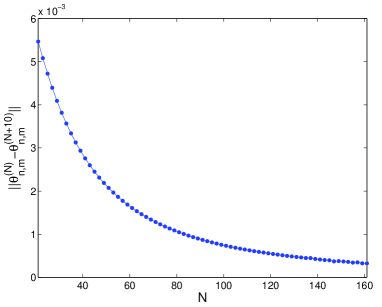
Figure 1: (Left panel) The spatial profile of the difference between the computed angles and the seed angles in a $81\times 81$ lattice at the AC-limit. (Right panel) Dependence of $||\theta_{n,m}^{N}-\theta_{n,m}^{N+10}||_{\infty}$ with respect to the lattice size $N$. In both cases, the lattice has fixed end boundary conditions.

Figure 2 shows the complementary norm of the $S=1$ and $S=2$ vortices, which is defined as [30]:

$$P=\sum_{n}\sum_{m}\left(|\phi_{\infty}|^{2}-|\phi_{n,m}|^{2}\right)$$ (14)

with $|\phi_{\infty}|^{2}$ being the background density; in our case, $|\phi_{\infty}|^{2}=1$. As it can be observed in the figure, vortices with $S=1$ and $S=2$ can be continued for couplings up to O$(1)$ and presumably for all $C$. It should be mentioned in passing that the method has also been successfully used to perform continuation in the vicinity of the anti-continuum limit, even for higher charge vortices such as $S=3$. Notice also that all the considered solutions are “black” solitons, i.e., the vortex center has amplitude $R_{0,0}=0$.

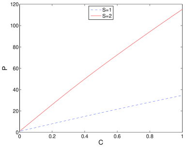
Figure 2: Dependence of the complementary norm on the coupling strength $C$ for $S=1$ and $S=2$.

Figures 3 and 4 show, for $S=1$ and $S=2$ vortices, respectively, the profile $|\psi_{n,m}|^{2}=|\phi_{n,m}|^{2}=R_{n,m}^{2}$, the angles $\theta_{n,m}$, the spectral plane of the stability eigenfrequencies and a comparison with the angles $\alpha_{n,m}$. In all cases, $C=0.2$ is shown, which corresponds to unstable vortices.

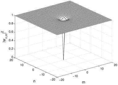
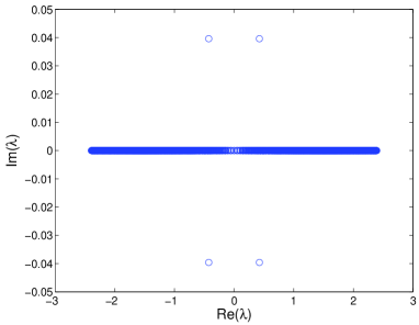
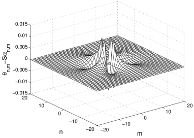
Figure 3: Vortex soliton with $S=1$ and $C=0.2$. (Top left panel) density Profile; (top right panel) angular dependence; (bottom left panel) spectral plane of stability eigenfrequencies [recall that the presence of eigenfrequencies with non-vanishing imaginary part denotes instability]; (bottom right panel) comparison of the vortex angles with $\alpha_{n,m}$.

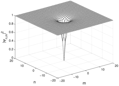
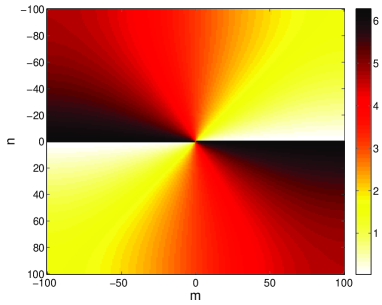
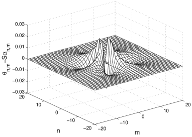
Figure 4: Same as Fig. 3 but for $S=2$.

The vortices with $S=1$ and $S=2$ are, respectively, stable for $C<C_{cr}\approx 0.0395$ and $C<C_{cr}\approx 0.0425$. This instability, highlighted in the case of the $S=1$ vortex in Fig. 5 can be rationalized by analogy with the corresponding stability calculations in the case of dark solitons [26]. In particular, the relevant linearization problem can be written in the form:

$$\lambda\left(\begin{array}[]{c}p_{n,m}\\ q_{n,m}^{\star}\end{array}\right)=\left(\begin{array}[]{cc}2|\phi_{n,m}|^{2}-1-C\Delta&\phi_{n,m}^{2}\\ -(\phi_{n,m}^{2})^{\star}&1-2|\phi_{n,m}|^{2}+C\Delta\end{array}\right)\left(\begin{array}[]{c}p_{n,m}\\ q_{n,m}^{\star}\end{array}\right).$$ (21)

However, by analogy to the corresponding 1d problem, the symmetry and the high spatial localization of the localized eigenvector at low coupling renders it a good approximation to write for the relevant perturbations that $\Delta p_{n,m}\approx-4p_{n,m}$ (and similarly for $q$), by virtue of which it can be extracted that the relevant eigenfrequency is $\lambda\approx 1-4C$. This leading order prediction (as a function of $C$) for the internal (“translational”) mode frequency is based on the anti-symmetry of both the real and the imaginary parts of the vortex configuration around its central site, in analogy with the anti-symmetry of the on-site dark soliton around its central site in the 1d analog of the problem [26, 27]. This feature (whose continuation to the $C\rightarrow\infty$ leads to a zero frequency mode due to the translational invariance of the underlying continuum model) is an example of the “negative energy” modes that both dark solitons (see e.g., [31] and references therein) and vortices (see e.g. [32]) are well-known to possess (due to the fact that, although stationary, they are not ground states of the respective 1d and 2d systems).

On the other hand, by analogy to the one dimensional calculation, it is straightforward to compute the dispersion relation characterizing the eigenfrequencies of the continuous spectrum (using $\{p_{n,m},q_{n,m}^{\star}\}=\{P,Q^{\star}\}\exp[i(k_{n}n+k_{m}m)]$, deriving a $2\times 2$ homogeneous linear system for $P$ and $Q$ and demanding that its determinant be zero) as extending through the interval $\lambda\in[-\sqrt{64C^{2}+16C},\sqrt{64C^{2}+16C}]$. Therefore, the collision of the point spectrum (negative energy) eigenvalue with the band edge of the continuous spectrum yields a prediction for the critical point of $C_{cr}\approx(2\sqrt{3}-3)/12\approx 0.0387$ in good agreement with the corresponding numerical result above. At $C=C_{cr}$ the system experiences a Hamiltonian Hopf bifurcation. In consequence, there exists an eigenvalue quartet $\{\lambda,\lambda^{*},-\lambda,-\lambda^{*}\}$. When $C$ increases, a cascade of Hopf bifurcations takes place due to the interaction of a localized mode with extended modes, as it was observed in one-dimensional dark solitons [26] (see also [33], [34] to illustrate the appearance of this phenomenon in Klein–Gordon lattices). This cascade implies the existence of stability windows between inverse Hopf bifurcations and direct Hopf bifurcations. For $S=1$ vortices, each one of the bifurcations takes place for decreasing $|{\rm Re}(\lambda)|$ when $C$ grows, and, in consequence, the bifurcations cease at a given value of $C$, as $|{\rm Re}(\lambda)|$ of the localized mode is smaller than that of the lowest extended mode frequency [however, in the infinite domain limit, this eventual restabilization would not take place but for the limit of $C\rightarrow\infty$]. This fact is illustrated in Fig. 5. A similar plot for the case of the $S=2$ vortex is shown in Fig. 6. When the lattice size tends to infinity ($N\rightarrow\infty$), the linear mode band extends from zero to infinity and becomes dense; thus, these stabilization windows should disappear at this limit. To illustrate this point, we have considered lattices of up to $201\times 201$ sites for the $S=1$ and $S=2$ vortices and have shown the growth rate of the corresponding instabilities in Fig. 7. The maximum growth rate (i.e. the largest imaginary part of the stability eigenfrequencies) takes place at $C\approx 0.115$ for $S=1$ and $S=2$ and being ${\rm Im}(\lambda)\approx 0.0845$ (0.0782) for $S=1$ ($S=2$).

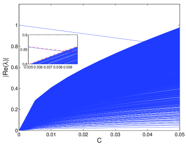
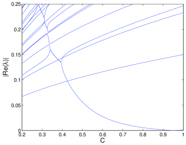
Figure 5: Real part of the stability eigenfrequencies for $S=1$. The panels show zooms of two different regions. Dashed lines correspond to the predicted eigenvalues $\lambda\approx 1-4C$ and $\lambda\approx\sqrt{64C^{2}+16C}$.

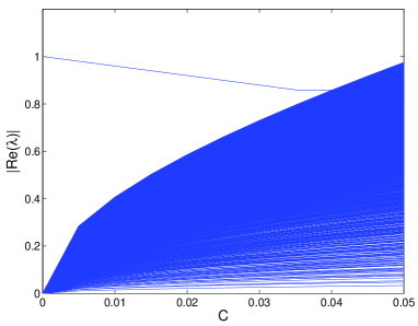
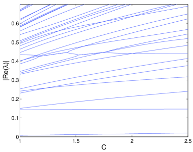
Figure 6: Real part of the stability eigenfrequencies for $S=2$. The panels show zooms of two different regions.

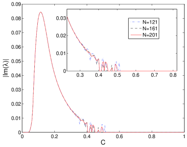
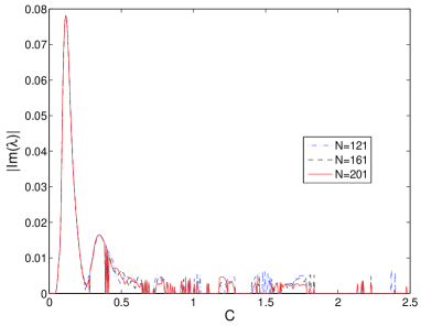
Figure 7: Imaginary part of the stability eigenfrequencies for $S=1$ (left panel) and $S=2$ (right panel), as a function of the coupling strength $C$. This corresponds to the growth rate of the corresponding instability.

4 Harmonic Trap

In this section, we consider the effect of introducing a harmonic trap. Thus, Eq. (2) is modified:

$$C\,\Delta\phi_{n,m}+(1-|\phi_{n,m}|^{2}-V_{n,m})\phi_{n,m}=0,$$ (22)

with the parabolic potential of the form

$$V_{n,m}=\frac{1}{C}\Omega^{2}r_{n,m}^{2}\ .$$ (23)

Fig. 8 shows a typical example of such a discrete vortex structure in the presence of an external trapping potential. The method presented in Section 2 is again used and converges unhindered by the presence of the magnetic trap. Notice that to include the trapping effect of the potential, we only modify the initial guess proposed in Section 2 through multiplying it by the so-called Thomas-Fermi profile of $\sqrt{\max(0,1-V_{n,m})}$ [1, 2]; the resulting guess converges even for small values of $C$ (such as the one used in Fig. 8). These vortices can be continued up to $C\rightarrow\infty$ and will converge to the corresponding continuum trapped vortices (for a recent discussion of such vortices in the presence of external potentials see e.g. [35]).

The stability of such structures is also examined in Figs. 9 and 10. The sole type of instability observed is an oscillatory one, with alternating windows of destabilization and restabilization. However, since the harmonic trap is well-known [1, 2] to discretize the spectrum of excitations, these windows of instability/restabilization are “true” ones (due to collisions of the “negative energy” mode of the vortex with the point spectrum of the background), rather than artificial ones (caused by the finite size of the computational domain). In fact, in this case, the maximum imaginary part of the eigenvalues does not depend on the number of grid points used (provided that the domain “encompasses” the harmonically trapped vortex). For high enough $C$, the charge $S=1$ vortex is always found to stabilize [32, 35]. It is interesting to also note that although the fundamental destabilization scenario indicated by the right panel of Fig. 9 has very strong parallels with its untrapped analog, the left panel of the figure indicates multiple additional collisions for smaller values of $C$. The negative Krein sign of the translational eigenvalue, discussed previously, suggests that these collisions should also result in oscillatory instabilities, although this is not discernible in the left column of Fig. 9. A relevant clarification to this apparent paradox is provided by Fig. 10 which clearly illustrates that the oscillatory instabilities do indeed arise but, in fact, emerge and disappear (the latter through inverse Hopf bifurcations) over very tiny parametric intervals of $C$ (and are, thus, apparently invisible over the scale of Fig. 9).

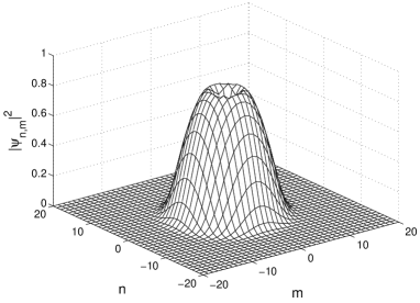
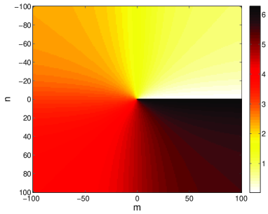
Figure 8: Vortex soliton with $S=1$ and $C=0.5$ in a harmonic trap with $\Omega=0.1$. (Left panel) density Profile; (Right panel) angular dependence.

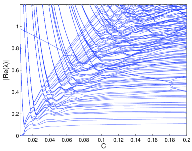
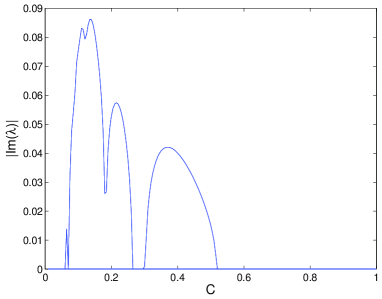
Figure 9: Real part (left panel) and imaginary part (right panel) of the stability eigenfrequencies for $S=1$ as a function of the coupling strength $C$ and a harmonic trap with $\Omega=0.1$.

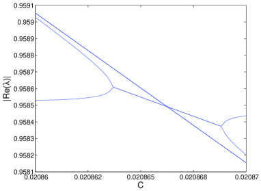
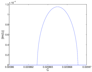
Figure 10: Same as Fig. 9 with a zoom around the first bifurcation. From this figure, it is clear that there is a Hopf bifurcation that destabilizes the vortex and an inverse Hopf. This pair of bifurcations takes place in a small interval of $C$ with a length of approximately $3\times 10^{-6}$.

5 Conclusions and Future Directions

In the present paper, we examined the discrete analog of continuum defocusing vortices which are perhaps the prototypical coherent structure in the two-dimensional nonlinear Schrödinger equation. We illustrated how to systematically obtain such structures through an appropriate continuation of the amplitude and phase profiles from the anti-continuum limit, and also discussed how to perform such a continuation from the continuum limit (at least for single core vortices). Such a continuation as a function of the coupling strength revealed significant analogies between these defocusing discrete vortices and their 1d analog of the discrete dark solitons, which are stable from coupling $C=0$ up to a critical coupling and are subsequently unstable for all higher couplings up to $C\rightarrow\infty$ (when they become restabilized). Something similar was observed and quantified in the case of discrete vortices. In addition to the most fundamental structures of topological charge $S=1$, structures of higher charge such as $S=2$ were obtained by similar means.

A natural topic for a more detailed future study arising from the present work concerns the understanding of multi-vortex bound states and their stability properties, as well as their detailed continuation as a function of the coupling and eventual disappearance as the coupling becomes sufficiently large. Another possible direction would be to examine such defocusing vortices in multi-component models (in analogy e.g., to the bright discrete vortices of [36]; see also references therein). There it would be of interest to study the similarities and differences of bound states of the same charge versus ones of, say, opposite charges. For these more demanding computations (as well as possibly ones associated with the 3d version of the present model [37]), more intensive numerical computations will be needed which may be aided by virtue of parallel implementation [38]. Such studies are currently in progress and will be reported in a future publication.

References

- [1] C.J. Pethick and H. Smith, Bose-Einstein condensation in dilute gases, Cambridge University Press (Cambridge, 2002).
- [2] L.P. Pitaevskii and S. Stringari, Bose-Einstein Condensation, Oxford University Press (Oxford, 2003).
- [3] M. R. Matthews, B. P. Anderson, P. C. Haljan, D. S. Hall, C. E. Wieman, and E. A. Cornell, Vortices in a Bose-Einstein condensate, Physical Review Letters 83, 2498-2501 (1999).
- [4] K. W. Madison, F. Chevy, W. Wohlleben, and J. Dalibard, Vortex Formation in a stirred Bose-Einstein condensate, Physical Review Letters 84, 806-809 (1999).
- [5] S. Inouye, S. Gupta, T. Rosenband, A. P. Chikkatur, A. Görlitz, T. L. Gustavson, A. E. Leanhardt, D. E. Pritchard, and W. Ketterle, Observation of vortex phase singularities in Bose-Einstein condensates, Physical Review Letters 87, 080402, 4 pages (2001).
- [6] J.R. Abo-Shaeer, C. Raman, J.M. Vogels, W. Ketterle, Observation of vortex lattices in Bose-Einstein condensates Science 292, 476-479 (2001).
- [7] J.R. Abo-Shaeer, C. Raman, W. Ketterle, Formation and decay of vortex lattices in Bose-Einstein condensates at finite temperatures Physical Review Letters 88, 070409, 4 pages (2002).
- [8] P. Engels, I. Coddington, P.C. Haljan and E.A. Cornell, Nonequilibrium effects of anisotropic compression applied to vortex lattices in Bose-Einstein condensates, Physical Review Letters 89, 100403, 4 pages (2002).
- [9] L.M. Pismen, Vortices in nonlinear fields, Oxford University Press (Oxford, 1999)
- [10] A.L. Fetter and A.A. Svidzinsky, J. Phys. Condens. Matter 13, R135 (2001).
- [11] P.G. Kevrekidis, R. Carretero-González, D.J. Frantzeskakis and I.G. Kevrekidis, Mod. Phys. Lett. B 18, 1481 (2004).
- [12] P.G. Kevrekidis, D.J. Frantzeskakis and R. Carretero-González (Eds.), Emergent Nonlinear Phenomena in Bose-Einstein Condensates, Springer-Verlag (Heidelberg, 2008).
- [13] N.G. Berloff, Quantum vortices, travelling coherent structures and superfluid turbulence, preprint available at: http://www.damtp.cam.ac.uk/user/ngb23.
- [14] R. Carretero-González, D.J. Frantzeskakis and P.G. Kevrekidis, Nonlinear waves in Bose-Einstein condensates: physical relevance and mathematical techniques, preprint available at: http://www-rohan.sdsu.edu/rcarrete/
- [15] V.A. Brazhnyi and V.V. Konotop, Mod. Phys. Lett. B 18, 627 (2004).
- [16] O. Morsch and M. Oberthaler, Rev. Mod. Phys. 78, 179 (2006).
- [17] P.G. Kevrekidis, R. Carretero-González, G. Theocharis, D.J. Frantzeskakis and B.A. Malomed, J. Phys. B 36, 3467 (2003).
- [18] A. Trombettoni and A. Smerzi, Phys. Rev. Lett. 86, 2353 (2001).
- [19] F.Kh. Abdullaev, B.B. Baizakov, S.A. Darmanyan, V.V. Konotop and M. Salerno, Phys. Rev. A 64, 043606 (2001).
- [20] G.L. Alfimov, P.G. Kevrekidis, V.V. Konotop and M. Salerno, Phys. Rev. E 66, 046608 (2002).
- [21] F.Kh. Abdullaev, Yu.V. Bludov, S.V. Dmitriev, P.G. Kevrekidis, and V. V. Konotop, Phys. Rev. E 77, 016604 (2008)
- [22] T. Pertsch, U. Peschel, F. Lederer, J. Burghoff, M. Will, S. Nolte and A. Tünnermann, Opt. Lett. 29, 468 (2004).
- [23] A. Szameit, J. Burghoff, T. Pertsch, S. Nolte, A Tünnermann, Opt. Express 14, 6055 (2006).
- [24] A. Szameit, Y. Kartashov, F. Dreisow, M. Heinrich, V.A. Vysloukh, T. Pertsch, S. Nolte, A. Tünnermann, F. Lederer and L. Torner, arXiv:0802.3196.
- [25] E. Smirnov, C.E. Rüter, M. Stepić, D. Kip and V. Shandarov, Phys. Rev. E 74, 065601 (R).
- [26] M Johansson and YuS Kivshar. Phys. Rev. Lett. 82, 85 (1999).
- [27] E.P. Fitrakis, P.G. Kevrekidis, H. Susanto and D.J. Frantzeskakis, Phys. Rev. E 75, 066608 (2007).
- [28] NG Berloff. J. Phys. A: Math. Gen. 37, 1617 (2004).
- [29] RS MacKay and S Aubry. Nonlinearity 7, 1623 (1994).
- [30] A Maluckov, L Hadžievski and BA Malomed. Phys. Rev. E 76, 046605 (2007).
- [31] G. Theocharis, P.G. Kevrekidis, M.K. Oberthaler, and D.J. Frantzeskakis, Phys. Rev. A 76, 045601 (2007).
- [32] H. Pu, C.K. Law, J.H. Eberly, and N. P. Bigelow,Phys. Rev. A 59, 1533 (1999); Y. Kawaguchi and T. Ohmi, Phys. Rev. A 70, 043610 (2004); J.A.M. Huhtamäki, M. Mötönen and S.M.M. Virtanen, Phys. Rev. A 74, 063619 (2006).
- [33] JL Marín and S Aubry. Physica D 119, 163 (1998).
- [34] A Álvarez, JFR Archilla, J Cuevas and FR Romero. New J. Phys. 4, 72 (2002).
- [35] K.J.H. Law, L. Qiao, P.G. Kevrekidis and I.G. Kevrekidis, Phys. Rev. A 77, 053612 (2008).
- [36] P.G. Kevrekidis and D.E. Pelinovsky, Proc. Roy. Soc. A 462, 2671 (2006).
- [37] P.G. Kevrekidis, B.A. Malomed, D.J. Frantzeskakis and R. Carretero-González, Phys. Rev. Lett. 93, 080403 (2004). R. Carretero-González, P.G. Kevrekidis, B.A. Malomed and D.J. Frantzeskakis, Phys. Rev. Lett. 94, 203901 (2005).
- [38] F Palmero. Breathers in Quantum Lattices. In P Alberigo, G Erbacci and F Garofalo, Eds. Science and Supercomputing in Europe (report 2005) , pages 758-762. CINECA, Bologna (Italy), 2006.