Electronic structure of edge and vortex states in chiral mesoscopic superconductor.

Abstract

We study a subgap quasiparticle spectrum in a mesoscopic disk of chiral superconductor. We find an exact expression for the spectrum of surface states localized at the disk edge. Considering an Abrikosov vortex placed at the center of a superconducting disk we investigate the spectrum transformation near the intersection points of surface and vortex anomalous energy branches . The resulting splitting of the anomalous branches due to the hybridization of edge and vortex states is determined by an external magnetic field and can lead in particular to the formation of a set of minigaps in the quasiparticle spectrum. Tuning the external magnetic field makes it possible to control the width of minigaps and the positions of corresponding density of states singularities at the minigaps edges.

1. Introduction. Recently, a considerable attention has been devoted to the investigation of a chiral superconducting state which is proposed to realize in p-wave triplet superconductor $Sr_{2}RuO_{4}$ (see Ref. Pwave and references therein). The chiral superconductivity can be associated with a formation of Cooper pairs with a non-zero orbital angular momentum. In this case a value of chirality $\chi$ is determined as a projection of the angular momentum of Cooper pairs on the $z$ axis. Generally, the superconducting order parameter is triplet (singlet) for odd (even) chirality $\chi$ and is given by $\hat{\Delta}=\Delta_{0}e^{i\chi\theta_{p}}\check{\sigma}_{z}$ and $\hat{\Delta}=\Delta_{0}e^{i\chi\theta_{p}}$ correspondinglyVolovik , where $\Delta_{0}$ is a bulk superconducting gap and $\check{\sigma}_{z}$ is a conventional spin operator. For $\chi\neq 0$ the phase of the order parameter depends on the direction of the electron momentum in $xy$ plane: ${\bf p}=p(\cos\theta_{p},\sin\theta_{p})$. The important consequence of this fact is an existence of surface Andreev bound statesHu ; Tanaka . They appear in the vicinity of scattering interfaces between a superconductor and an insulator, if the order parameter phase takes different values for the incident and reflected quasiparticles (QP) with different momentum directions. The formation of Andreev bound states increases the local density of states at the surface of a superconductor resulting in zero-bias a conductance peak anomaly observed in tunneling spectroscopy of high-$T_{c}$ cuprates with a d-wave symmetry of superconducting pairing Guy as well as in p-wave triplet superconductor $Sr_{2}RuO_{4}$ Fogel .

Under an applied magnetic field, generating screening current and vortices the spectrum of surface states acquires a Doppler shift, leading to the splitting of the zero-bias conductance peak Iniotakis1 . Recently in work Iniotakis2 it was proposed that the Doppler shift effect should lead to the chirality selective influence of the magnetic field on the surface states in chiral p-wave superconductor ($|\chi|=1$), such as $Sr_{2}RuO_{4}$. The QP density of states (DOS) near the flat surface was shown to depend on the orientation of the magnetic field with respect to the $z$ axis as well as on the vorticity in case when an Abrikosov vortex is pinned near the surface of a superconductor.

If an Abrikosov vortex is situated close to the boundary of a superconductor, then in addition to the Doppler shift effect Iniotakis2 it is necessary to take into account the hybridization of edge modes and low–energy vortex core states CdGM . In this case spectrum modification is determined by the overlapping of QP wave functions localized near the surface and near the vortex core. The characteristic localization length of subgap QP wave functions is determined by a superconducting coherence length $\xi$. Therefore the hybridization of vortex and edge states should be particularly important in mesoscopic superconducting samples of the size of several $\xi$.

Let us consider a model problem when a superconducting sample has ideal disk geometry in $xy$ plane. In this case the spectrum of edge states can be expressed in terms of the angular momentum $\mu$ which is conserved due to the axial symmetry. We assume the validity of a quasiclassical approach so that one can consider QP motion along trajectories, i.e. straight lines along the direction of QP momentum ${\bf p}=p(\cos\theta_{p},\sin\theta_{p})$. Employing analogy with a point Josephson junction the spectrum of surface states can be written as follows: $E_{s}=-\Delta_{0}\cos(\Delta\varphi/2)$, where $0<\Delta\varphi<2\pi$ is the difference between gap function phases seen by the incident and reflected QPs. Under the reflection of a trajectory at the disk boundary the angle $\theta_{p}$ transforms as $\theta_{p}\rightarrow\theta_{p}+\pi+2\arcsin(b/R)$, where $b=-\mu/k_{F}$ is a continuous impact parameter, i.e. a distance from the trajectory to the disk center, $k_{F}$ is a Fermi wave number and $R$ is a disk radius. In case when there is no circulating superconducting currents we obtain $\Delta\varphi=\left[\chi(\pi+2\arcsin(b/R))\right]\mod(2\pi)$ yielding a set of anomalous energy branches corresponding to the edge states VolovikEdge ; Stone :

$$E_{sj}(\mu)\approx-(\mu-\mu_{j})\omega_{sj},$$ (1)

where $j=1...|\chi|$ and $\mu_{j}=(k_{F}R)\sin(\pi n_{j}/2\chi)$. The integer index $n_{j}$ from the interval $-|\chi|<n_{j}<|\chi|$ is chosen so that the combination $\chi-n_{j}$ to be odd. As noted in Ref.VolovikEdge the spectrum of edge states (1) is analogous to the general spectrum of quasiparticles localized within a vortex core multi-spectrum-num . The interlevel spacing for a particular anomalous branch $\omega_{sj}=\chi\Delta_{0}/(k_{F}R\cos(\pi n_{j}/2\chi))$ is much smaller than the bulk superconducting gap $\Delta_{0}$ provided $k_{F}R\gg 1$, therefore the anomalous branches can be considered as functions of a continuous impact parameter $b=-\mu/k_{F}$. In case of even chirality $\chi$ all energy branches cross the Fermi level at finite impact parameters $b=-\mu_{j}/k_{F}$, and for the odd $\chi$ there exists an energy branch with $\mu_{j}=0$, crossing the Fermi level at $b=0$.

If an Abrikosov vortex is placed at the center of a superconducting disk there appears another anomalous energy branch associated with the spectrum of vortex states CdGM :

$$E_{v}(\mu)=-\mu\omega_{v}.$$ (2)

Here $\omega_{v}\sim\eta\Delta_{0}/(k_{F}\xi)$, where $\xi=\hbar V_{F}/\Delta_{0}$ is a superconducting coherence length and $V_{F}=\hbar k_{F}/m$ is a Fermi velocity. The value of vorticity $\eta=\pm 1$ is determined by a sign of the superfluid velocity circulation in the counterclockwise direction around the vortex core. The angular momentum $\mu$ in Eq.(2) is integer (half–integer) for the odd (even) chirality value Volovik .

Considered as continuous functions of a quasiclassical impact parameter $b=-\mu/k_{F}$ the spectrum branches $E_{v}(b)$ and $E_{sj}(b)$ intersect at the certain points $b=b_{j}$. The splitting of energy levels at the degeneracy point occurs due to the hybridization of vortex and edge states and can be estimated using the perturbation method for an almost degenerate two-level system (see Ref.LL ), which yields the secular equation:

$$[E-E_{sj}(b)][E-E_{v}(b)]=J^{2},$$ (3)

where the factor $J$ is determined by the overlapping of the corresponding wave functions. Using a Taylor expansion $E_{v}(b)=E_{v}(b_{j})+E^{\prime}_{v}(b_{j})(b-b_{j})$ and $E_{sj}(b)=E_{sj}(b_{j})+E^{\prime}_{sj}(b_{j})(b-b_{j})$ one can see that the scenario of branch splitting depends on the slopes of energy branches $E^{\prime}_{v}=dE_{v}/db$ and $E^{\prime}_{sj}=dE_{sj}/db$ at the intersection point $b=b_{j}$. In case when the signs of the slopes are opposite there appears a minigap in the QP spectrum. The minigap width i.e. the minimal energy spacing between QP levels corresponding to the different energy branches can be found from Eq.(3) as follows:

$$\delta E=2|J|\;\sqrt{|E^{\prime}_{v}E^{\prime}_{sj}|}/\left(|E^{\prime}_{v}|+|E^{\prime}_{sj}|\right).$$ (4)

Otherwise, when $E^{\prime}_{v}$ and $E^{\prime}_{sj}$ have the same sign,the minigap width is always equal to zero. Generally the energy branches $E_{v}(b)$ and $E_{sj}(b)$ cross at $|b_{j}|\sim\xi$ and $|E|\sim\Delta_{0}$, where the spectra are not described by the expressions (1,2). For the sake of simplicity further we focus on a particular case of chiral p–wave superconductor with $|\chi|=1$. Then there is only one anomalous surface energy branch $E_{s}(b)$, crossing the Fermi level at $b=0$ simultaneously with the vortex energy branch $E_{v}(b)$. Therefore the spectrum transformation takes place within a domain of small energies $|E|\ll\Delta_{0}$, where the surface and vortex states are well localized and the overlapping factor can be evaluated as follows $|J|\sim\Delta_{0}e^{-R/\xi}$. In this case the splitting of energy branches is shown schematically in Fig.(1) for the opposite and equal signs of chirality $\chi$ and vorticity $\eta$.

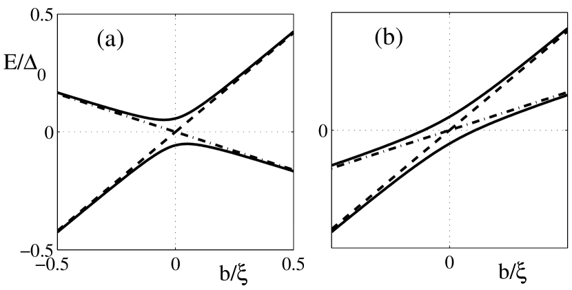
Figure 1: FIG. 1 Shown by solid lines is the spectrum transformation caused by the interaction of vortex and surface spectrum branches: (a) chirality and vorticity have different signs ($\eta=1$, $\chi=-1$); (b) chirality and vorticity have the same signs ($\eta=1$, $\chi=1$). The dash and dash-dotted curves correspond to the non–interacting vortex and surface energy branches.

Following Ref. Iniotakis2 one could expect the surface energy branch $E_{s}(b)$ to be modified due to a Doppler shift induced by a superfluid velocity circulating around the vortex core. However, it is not the case if $|\chi|=1$ when the Doppler shift is totally compensated by an additional vortex–induced difference of the order parameter phase for the incident and reflected QP. Indeed, in the presence of a vortex–induced superfluid velocity ${\bf v_{s}}$ the Doppler shifted spectrum of surface states is given by: $E_{s}=-\Delta_{0}\cos(\Delta\varphi/2)+{\bf p_{F}}\cdot{\bf v_{s}}$, where ${\bf p_{F}}\cdot{\bf v_{s}}=-\eta\Delta_{0}(b/R)$ is a Doppler shift energy at the disk edge and the phase difference is $\Delta\varphi\approx\pi+2(\chi+\eta)b/R$. It is easy to see that for $|\chi|=1$ the surface energy branch is still given by Eq.(1) with $n_{j}=0$.

2. Model. In order to investigate in detail the effects described above we proceed with a quantitative analysis of the QP spectrum in chiral superconductor on the basis of Bogoulubov - de Gennes theory:

$$\hat{H}_{0}\Psi+\left(0\quad\;\,\hat{\Delta}\atop\hat{\Delta}^{+}\quad 0\right)\Psi=E\Psi\ ,$$ (5)

where $\hat{H}_{0}=\check{\tau}_{3}[\left(i\hbar\nabla+e\check{\tau}_{3}{\bf A}/c\right)^{2}-p_{F}^{2}]/2m$, $\Psi=(u,v)$, $u$ and $v$ are the amplitudes of the electron and hole components, $\check{\tau}_{i}$ are the Pauli matrices in a particle–hole space, $\hat{\Delta}$ is a gap operator:

$$\hat{\Delta}=\left\{\Delta(\hat{\bf{r}}),e^{i\chi\theta_{p}}\right\},$$ (6)

where $\hat{\bf{r}}$ is a coordinate operator, $\Delta({\bf{r}})$ describes the spatial dependence of the gap function and $\{A,B\}=AB+BA$ is an anticommutator which provides the gauge invariance of $\hat{\Delta}$. Here we omit the spin–dependent part of the gap operator $\hat{\Delta}$, neglecting the spin–orbit interaction. Also we neglect the dispersion of QP energy in the direction perpendicular to the anisotropy plane $xy$, assuming a cylindrical Fermi surface. The magnetic field is directed along the $z$ axis ${\bf H}=-H{\bf z}_{0}$ and for extreme type-II superconductors we can consider the magnetic field to be homogeneous on the spatial scale $R$ and take the gauge ${\bf A}=[{\bf H},{\bf r}]/2$. Within the quasiclassical approach the wave function in the momentum representation can be taken in the form:

$$\Psi({\bf p})=\frac{2\pi}{k_{F}}\int\limits_{-\infty}^{+\infty}dse^{-i(|{\bf p}|-\hbar k_{F})s/\hbar}\psi(s,\theta_{p})\ ,$$ (7)

where $s$ is a coordinate along a trajectory. In $(s,\theta_{p})$ representation the expression for the coordinate operator in Eq.(6) has the following form:

$$\hat{\bf r}=s{\bf k}_{F}/k_{F}+\left\{[{\bf k}_{F},{\bf z}_{0}],\hat{\mu}\right\}/(2k_{F}^{2}),$$ (8)

where $\hat{\mu}=-i\partial/\partial\theta_{p}$ is an angular momentum operator. The equation for $\psi(s,\theta_{p})$ along a quasiclassical trajectory reads:

$$-i\check{\tau}_{3}\hbar V_{F}\frac{\partial}{\partial s}\psi+\left(0\quad\;\,\hat{\Delta}\atop\hat{\Delta}^{+}\quad 0\right)\psi=\left(E+\hat{\mu}\,\frac{\hbar\omega_{H}}{2}\right)\psi,$$ (9)

where $\omega_{H}=|e|H/mc$ is a cyclotron frequency. The terms quadratic in $H$ were neglected in (9) because we consider the distances much smaller than the cyclotron radius $r_{H}=V_{F}/\omega_{H}$. The wave function in the real space is expressed from Eq.(7) in the following way (see Refs. PRB2007 ,MS2006 ):

$$\Psi(r,\theta)=\int_{0}^{2\pi}d\theta_{p}e^{ik_{F}r\cos(\theta-\theta_{p})}\psi(r\cos(\theta-\theta_{p}),\theta_{p}).$$ (10)

For an ideal disk it is convenient to use a polar coordinate system $(r,\theta)$ with the origin at the disk center. Then, the boundary condition at the surface of a superconducting disk of the radius $R$ reads:

$$\Psi(R,\theta)=0.$$ (11)

3. Spectrum of edge states. At first we investigate the spectrum of edge states solving Eq.(9) with spatially homogeneous order parameter distribution: $\Delta({\bf r})=\Delta_{0}$ and applying the boundary condition (11). Due to the axial symmetry of the superconducting sample we separate the $\theta_{p}$ and $s$ variables in Eq.(9):

$$\psi(s,\theta_{p})=e^{i\mu\theta_{p}+i\chi\check{\tau}_{3}\theta_{p}/2}G_{\mu}(s),$$ (12)

where $\mu=n+\chi/2$ is an angular momentum, and $n$ is integer. The function $G_{\mu}$ satisfies the following equation:

$$-i\check{\tau}_{3}\hbar V_{F}\frac{\partial}{\partial s}G_{\mu}+\Delta_{0}\check{\tau}_{1}G_{\mu}=\tilde{E}G_{\mu},$$ (13)

where $\tilde{E}=E+\mu\,(\hbar\omega_{H}/2)$. In order to apply the boundary conditions (11) we evaluate the integral in (10) using the stationary phase method. For a given $\mu$ we obtain:

$$\Psi(R,\theta)=e^{i(k_{F}s^{*}-\pi/4)}\psi(s^{*},\theta_{1})+e^{i(\pi/4-k_{F}s^{*})}\psi(-s^{*},\theta_{2}),$$

where $s^{*}=\sqrt{R^{2}-(\mu/k_{F})^{2}}$ and the stationary phase points are given by $\theta_{1}=\theta+\arcsin(\mu/k_{F}R)$ and $\theta_{2}=\theta+\pi-\arcsin(\mu/k_{F}R)$. Thus, we obtain the boundary condition for the function $G_{\mu}(s)$:

$$G_{\mu}(s^{*})=e^{i\alpha-i\check{\tau}_{3}\varphi}G_{\mu}(-s^{*}),$$ (14)

where $\alpha=\mu[\pi-2\arcsin(\mu/k_{F}R)]-2k_{F}s^{*}-\pi/2$ and $\varphi=\chi[\arcsin(\mu/k_{F}R)-\pi/2]$.

The general solution of Eq.(13) can be written as follows:

$$G_{\mu}=c\left(1\atop e^{i\gamma}\right)e^{qs/\xi}+d\left(1\atop e^{-i\gamma}\right)e^{-qs/\xi},$$ (15)

where $c,d$ are the scalar coefficients, $\gamma=\arccos(\tilde{E}/\Delta_{0})$ and $q=\sqrt{\Delta_{0}^{2}-\tilde{E}^{2}}/\Delta_{0}$. Then, from the boundary condition (14) we obtain the expression for the spectrum of edge states:

$$E=\Delta_{0}M/\sqrt{1+M^{2}}-\mu(\hbar\omega_{H}/2),$$ (16)

where $M=\coth(2qs^{*}/\xi)\cot\varphi-\cos\alpha/\sinh(2qs^{*}/\xi).$ It is possible to evaluate Eq.(16) to find an explicit expression for the energy levels lying much lower than the superconducting gap. For simplicity we start our analysis with the case of a zero magnetic field. Considering the low energies $|E|\ll\Delta_{0}$ we obtain that the spectrum consists of $|\chi|$ energy branches:

$$E_{sj}(\mu)=-(\mu-\mu_{j})\omega_{sj}+\Delta_{0}\frac{(-1)^{k_{j}}\cos\alpha}{\sinh(2s^{*}/\xi)},$$ (17)

where $\omega_{sj}=\chi\Delta_{0}\coth(2s^{*}/\xi)/(k_{F}R\cos(\pi n_{j}/2\chi))$ and $\mu_{j}=(k_{F}R)\sin(\pi n_{j}/2\chi)$. The integer index $n_{j}$ from the interval $-|\chi|<n_{j}<|\chi|$ is chosen so that the combination $\chi-n_{j}$ to be odd: $\chi-n_{j}=2k_{j}+1$. From Eq.(17) one can see that the energy levels are the oscillating functions of a disk radius with a period $\delta R=\pi/k_{F}$. The amplitude of energy levels oscillations is larger than the interlevel spacing provided the disk radius is smaller than the critical value $R_{c}$ determined by the condition $\omega_{sj}\sim\Delta_{0}/\sinh(2s^{*}/\xi)$. For the typical values of the parameter $k_{F}\xi\sim 10^{2}-10^{3}$ we obtain $R_{c}/\xi\sim 3-5$. Note that in case $|\chi|=1$ Eq.(17) is completely analogous to the expression obtained in Ref.MelnikovPrl for the spectrum of vortex core states modified by the normal reflection of QP at the surface of s-wave mesoscopic superconductor. At $R\gg R_{c}$ the exponentially small oscillating term in Eq.(17) can be omitted and we obtain the low–energy spectrum of surface states consistsing of a set of anomalous branches (1), similar to the spectrum of multiquantum vortex with a vorticity equal to $\chi$ multi-spectrum-num . Then, Eq.(17) describes an appearance of an energy band due to the interaction of surface states localized at the opposite ends of a trajectory $s=\pm s^{*}$. The bandwidth $\Delta_{0}/\sinh(2s^{*}/\xi)$ is proportional to the overlap of decaying wave functions of edge states.

Applying a magnetic field $H$ along the $z$ axis one introduces the shift of surface energy levels $\mu(\hbar\omega_{H}/2)$ in Eq.(17). In fact it is a Doppler shift effect due to the Meissner current flowing along the circumference of a superconducting disk. The same effect was studied in Ref.Iniotakis2 for the flat geometry of the superconducting sample boundary. Let us consider the expression (17) in more detail for the case of $|\chi|=1$. Taking into account the finite external magnetic field we obtain that the spectrum is given by Eq.(17) with $\omega_{s1}=\omega_{s}=\chi\Delta_{0}/(k_{F}R)+\hbar\omega_{H}/2$ and the phase of energy oscillations: $\alpha(\mu)=\mu\pi-2k_{F}R-\pi/2$. Note that $\alpha(\mu+2)=\alpha(\mu)+2\pi$, therefore the spacing between levels corresponding to the angular momentum values $\mu$ and $\mu+2$ is $2\omega_{s}$ and can be neglected within the quasiclassical consideration. On the other hand, the spacing between levels corresponding to $\mu$ and $\mu+1$ is $\Delta_{0}e^{-2R/\xi}\sin(2k_{F}R)$, which can be much larger than $\omega_{s}$ if $R<R_{c}$. Thus one can consider two continuous branches corresponding to the odd and even values of $n=\mu-1/2$:

$$E_{s}(b)=\omega_{s}k_{F}b\pm 2\chi\Delta_{0}e^{-2R/\xi}\sin(2k_{F}R),$$ (18)

where $b=-\mu/k_{F}$ is an impact parameter. At $R>\xi$, the Doppler shift energy $k_{F}b(\hbar\omega_{H}/2)$ in Eq.(18) can substantially change the slope of the branches $E_{s}(b)$. Indeed, $\hbar\omega_{H}\sim(H/H_{c2})\Delta_{0}/(k_{F}\xi)$, where $H_{c2}\sim\phi_{0}/\xi^{2}$ is the upper critical field and $\phi_{0}=\pi\hbar c/e$ is the magnetic flux quantum. Therefore the magnetic field of the magnitude $|H|>(\xi/R)H_{c2}$ can reverse the slope of $E_{s}(b)$. Particularly at $H=-2\chi\phi_{0}/(\xi R)$ we obtain a dispersionless energy branches $E_{s}=\pm 2\Delta_{0}e^{-2R/\xi}\cos(2k_{F}R)$. In the Fig.(2) we show one of the spectrum branches (for $\mu=2n+1/2$) given by Eq.(16) for the different values of magnetic field. Considering the measurable characteristics of the QP spectrum we obtain that the density of states (DOS) at the Fermi level $\nu(0)=1/|\omega_{s}|$ can be controlled tuning the magnitude and direction of an external magnetic field.

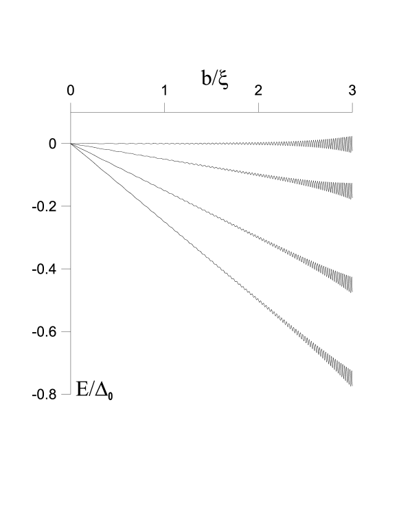
Figure 2: FIG. 1 Spectrum of surface states for $\chi=-1$ and $\mu=2n+1/2$. Curves from bottom to top correspond to the different values of magnetic field from $H=0$ to $H=2\phi_{0}/(\xi R)$ (corresponding to $\omega_{s}=0$). We choose $R=4\xi$ and $k_{F}\xi=200$.

Analyzing the influence of external magnetic field on the surface states spectrum we have neglected a magnetic field $H_{s}$ generated by the current, carried by the surface states. The density of this current is of the order of the critical one for depairing VolovikEdge ; Stone and it flows within the surface shell of the width $\xi$. Evaluating the magnetic field we obtain $H_{s}\sim(\xi/\lambda)^{2}H_{c2}$, where $\lambda$ is a London penetration length. Thus for extreme type–II superconductors ($\xi/\lambda\ll 1$) the field of the surface current can be neglected.

The considered model with a spatially homogeneous gap function $\Delta({\bf r})=\Delta_{0}$ is adequate only for not very large applied magnetic field. Generally, it does not work when the field is large enough to suppress a surface barrier preventing vortex entry $H_{c}\sim H_{c2}(\xi/R)$ Buzdin . Certainly, in our case a criterion for the vortex formation should be sensitive to the orientation of magnetic field with respect to the $z$ axis. Now we proceed with the analysis of the QP spectrum assuming that a vortex has already entered the sample and is placed at the center of a superconducting disk.

4. Vortex–induced spectrum transformation. In the vicinity of a vortex core the gap function has the following form: $\Delta({\bf r})=\Delta_{0}D_{v}(r)e^{i\eta\theta},$ where $\eta=\pm 1$ is the vorticity and $D_{v}(r)$ is a dimensionless vortex core profile. The gap operator $\hat{\Delta}$ in $(s,\theta_{p})$ representation has the following form:

$$\hat{\Delta}=\Delta_{0}\frac{D_{v}(s)}{2|s|}\left\{(s+\eta\hat{\mu}/k_{F}),e^{i(\chi+\eta)\theta_{p}}\right\}.$$ (19)

To be specific, we choose a model vortex core profile: $D_{v}(r)=r/\sqrt{r^{2}+\xi^{2}}$. Once again we can separate the $s$ and $\theta_{p}$ variables:

$$\psi(s,\theta_{p})=e^{i\mu\theta_{p}+i(\chi+\eta)\check{\tau}_{3}\theta_{p}/2}G_{\mu}(s),$$ (20)

where $\mu$ is integer. We will consider the trajectories passing close to the vortex core with impact parameters $b\ll\xi$, corresponding to $|\mu|\ll k_{F}\xi$. Then, from the boundary condition (11) we obtain Eq.(14) with $s^{*}=R$, $\alpha=\mu\pi-2k_{F}R-\pi/2$ and $\varphi=(\chi+\eta)[\mu/(k_{F}R)-\pi/2]$. The function $G_{\mu}(s)$ we satisfies the following equation:

$$-i\hbar V_{F}\check{\tau}_{3}\frac{\partial}{\partial s}G_{\mu}+{\bf U}(s)G_{\mu}=\left(\tilde{E}-\frac{\mu}{k_{F}\xi}{\bf W}(s)\right)G_{\mu}.$$ (21)

The matrices ${\bf U},{\bf W}(s)$ are defined at $-R<s<R$ as follows:

$${\bf U}(s)=\Delta_{0}D_{v}(s)\frac{s}{|s|}\check{\tau}_{1}$$

$${\bf W}(s)=\Delta_{0}D_{v}(s)\frac{\xi}{|s|}\check{\tau}_{2}$$

We assume that the size of the disk is rather large: $R>\xi$ therefore Eq.(21) together with the boundary condition (14) describe the interaction of vortex states localized near the vortex center i.e. $s=0$ and the edge states localized at $s=\pm R$. Thus, it is natural to use the tight–binding approximation of the wave function to calculate the spectrum. To this end we consider a continuation of the function $G_{\mu}(s)$ and coefficients ${\bf U},{\bf W}(s)$ of Eq.(21) to the whole axis $-\infty<s<\infty$ using the periodicity conditions:

$$G_{\mu}(s+2R)=e^{i\alpha-i\check{\tau}_{3}\varphi}G_{\mu}(s)$$

$${\bf U},{\bf W}(s+2R)=e^{-2i\check{\tau}_{3}\varphi}{\bf U},{\bf W}(s).$$

We find the solution of Eq.(21) as a superposition of the functions localized at $s_{n}=2nR$ corresponding to the vortex states and localized at $d_{n}=(2n+1)R$ corresponding to the surface states:

$$G_{\mu}=C_{1}\sum_{n}V_{n}+C_{2}\sum_{n}S_{n},$$ (22)

where $C_{1},C_{2}$ are the arbitrary coefficients and the generic terms are:

$$V_{n}(s)=e^{in(\alpha-\check{\tau}_{3}\varphi)}e^{-K_{v}(s-s_{n})}e^{i\check{\tau}_{3}\pi/4}\left(1\atop 1\right),$$

$$K_{v}(s-s_{n})=\int_{s_{n}}^{s}D_{v}(s-s_{n})\vartheta(s-s_{n})\frac{ds}{\xi}$$

and

$$S_{n}(s)=e^{in(\alpha-\check{\tau}_{3}\varphi)}e^{-K_{s}(s-d_{n})}e^{-i\check{\tau}_{3}\pi/4}\left(1\atop 1\right),$$

$$K_{s}(s-s_{n})=\int_{d_{n}}^{s}D_{v}(s-d_{n})\vartheta(s-d_{n})\frac{ds}{\xi}$$

where we have introduced the step function $\vartheta(s)=s/|s|$.

Following the standard tight binding method we substitute the solution in the form (22) into the Eq.(21), multiply by $V^{*}_{n}$ and $S^{*}_{n}$ from the left and integrate over $s$, taking into account the overlapping of the nearest neighbor functions. We omit here the details of calculation of the corresponding integrals which yields a linear system of equations for the coefficients $C_{1},C_{2}$:

$$\left[E-E_{v}(\mu)\right]C_{1}=-(i/2)e^{-R/\xi}(1-e^{-i\alpha})C_{2}$$

$$\left[E-E_{s}(\mu)\right]C_{2}=ie^{-R/\xi}(1-e^{i\alpha})C_{1}.$$ (23)

The solvability condition for this system is given by the Eq.(3) with $J=\sqrt{2}\Delta_{0}e^{-R/\xi}\sin(\alpha/2)$. The vortex energy branch $E_{v}(\mu)$ is given by (2) with $\omega_{v}\approx 0.84\eta\Delta_{0}/(k_{F}\xi)+\hbar\omega_{H}/2$ and the surface energy branch $E_{s}(\mu)$ is given by (1) with $n_{j}=0$ and $\omega_{s}\approx\chi\Delta_{0}/(k_{F}R)+\hbar\omega_{H}/2$.

According to the arguments presented in introduction in case when the vorticity $\eta$ and chirality $\chi$ are of the opposite signs [Fig.(1)a], there exists a minigap at the Fermi level. In this case the DOS has van Hove singularities at the minigap edges, i.e. at $E=\pm\delta E$. Applying the magnetic field $H$ along the $z$ axis one can change the slope of the intersecting branches $E_{v}(b)$ and $E_{s}(b)$ and therefore shift the positions of van Hove singularities according to the Eq.(4). For large enough magnetic fields $|H|>2\phi_{0}/(\xi R)$ the slope of energy branch $E_{s}(b)$ can be reversed. In this case as well as in case of the equal signs of vorticity $\eta$ and chirality $\chi$ the spectrum is gapless as shown on the [Fig.(1)b].

5. Effect of surface roughness. In conclusion we note that in previous sections we analyzed the electronic spectrum for a sample with the perfect surface. One can expect that the surface roughness would break the interference of QP waves and as a result the DOS singularity at the minigap edge would be smeared. However, it is not the case for a wide class of surface imperfections. Particularly, let us assume that the surface of the sample is described by the equation $r=R(\theta)$, where $R(\theta)$ is a smooth function fluctuating over an average value $r=R_{0}$, so that $|R(\theta)-R_{0}|\ll\xi$ and $|dR/d\theta|\ll\xi$. Then, following a procedure developed in Ref.PRB2007 one can find the solution of Eq.(9) in the form of expansion (22) with the angle–dependent coefficients $C_{1},C_{2}(\theta)$. Using a tight binding method we arrive at the system of differential equations for the functions $C_{1},C_{2}(\theta)$, which coincides with Eq.(Electronic structure of edge and vortex states in chiral mesoscopic superconductor.) if one takes $\hat{\mu}=-i\partial/\partial\theta$ and $e^{i\alpha}=-ie^{-ik_{F}(R(\theta)+R(\theta+\pi))}e^{i\pi\hat{\mu}}$. Considering the low–energy limit $|E|\ll\Delta_{0}$, it is natural to assume that the functions $C_{1,2}(\theta)$ consist of a limiting number of the lowest angular harmonics with $|\mu|\ll k_{F}\xi$. Thus, the coefficients of Eq.(Electronic structure of edge and vortex states in chiral mesoscopic superconductor.) can be averaged over the small angular interval to exclude higher angular harmonics of the rapidly oscillating exponent $e^{-ik_{F}(R(\theta)+R(\theta+\pi))}$. It is important that the right hand sides of equations in system (Electronic structure of edge and vortex states in chiral mesoscopic superconductor.) can not vanish after this averaging, in contrast to the analogous problem for the case of s–wave superconductorPRB2007 . The resulting spectrum should have the form (3) with $J=\beta\Delta_{0}e^{-R_{0}/\xi}$, where a factor $\beta\sim 1$ depends on the particular realization of the surface roughness.

I am grateful to G.E. Volovik for drawing my attention to this problem and to A.S. Melnikov for numerous stimulating discussions and help with preparation of this paper. Also it is my pleasure to thank E. Ezhova for help with numerical calculations and A. Aladyshkin for valuable remarks. The research was supported, in part, by Russian Foundation for Basic Research, by Program “Quantum Macrophysics” of RAS, and by Russian Science Support and “Dynasty” Foundations.

References

- (1) A. P. Mackenzie and Y. Maeno, Rev. Mod. Phys. 75, 657 (2003);
- (2) G. E. Volovik, JETP Lett., 70, 609 (1999);
- (3) C. R. Hu, Phys. Rev. Lett. 72, 1526 (1994).
- (4) Y. Tanaka and S. Kashiwaya, Phys. Rev. Lett. 74, 3451 (1995).
- (5) G. Deutscher, Rev. Mod. Phys., 77, 109 (2005);
- (6) F. Laube, G. Goll, H. V. Lohneysen, M. Fogelstrom, and F. Lichtenberg, Phys. Rev. Lett. 84, 1595 (2000); Z.Q. Mao, K.D. Nelson, R. Jin, Y. Liu, and Y. Maeno, Phys. Rev. Lett. 87, 037003 (2001).
- (7) S. Graser, C. Iniotakis, T. Dahm and N. Schopohl, Phys. Rev. Lett., 93, 247001 (2004);
- (8) T. Yokoyama, C. Iniotakis, Y. Tanaka, and M. Sigrist, cond-mat:0710.4204v1 (2007);
- (9) C. Caroli, P. G. de Gennes, J. Matricon, Phys. Lett. 9, 307 (1964);
- (10) G. E. Volovik, JETP Lett., 66, 522 (1997);
- (11) M. Stone and R. Roy, Phys. Rev. B 69, 184511 (2004);
- (12) D. Rainer, J. A. Sauls, and D. Waxman, Phys. Rev. B 54, 10094 (1996); S. M. M. Virtanen and M. M. Salomaa, Phys. Rev. B 60, 14581 (1999); A. S. Mel’nikov and V. M. Vinokur, Nature, 415, 60 (2002); Phys. Rev. B 65, 224514 (2002);
- (13) L. D. Landau, E. M. Lifshitz ”Quantum mechanics. Non-relativistic theory”, Pergamon Press, 1991;
- (14) N. B. Kopnin, A. S. Mel’nikov, V. I. Pozdnyakova, D. A. Ryzhov, I. A. Shereshevskii, and V. M. Vinokur, Phys. Rev. B, 75, 024514 (2007);
- (15) A. S. Mel’nikov, M.A. Silaev, JETP Lett., 83, 675 (2006);
- (16) N. B. Kopnin, A. S. Mel’nikov, V. I. Pozdnyakova, D. A. Ryzhov, I. A. Shereshevskii, and V. M. Vinokur, Phys. Rev. Lett. 95, 197002 (2005);
- (17) A. I. Buzdin, J. P. Brison, Phys. Lett. A 196, 267 (1994);