The normal distribution in some constrained sample spaces

Abstract

Phenomena with a constrained sample space appear frequently in practice. This is the case e.g. with strictly positive data and with compositional data, like percentages and the like. If the natural measure of difference is not the absolute one, it is possible to use simple algebraic properties to show that it is more convenient to work with a geometry that is not the usual Euclidean geometry in real space, and with a measure which is not the usual Lebesgue measure, leading to alternative models which better fit the phenomenon under study. The general approach is presented and illustrated both on the positive real line and on the $D$-part simplex.

1 Introduction

In general, any statistical analysis is performed assuming data to be realisations of real random vectors whose density functions are defined with respect to the Lebesgue measure, which is a natural measure in real space and compatible with its inner vector space structure. Sometimes, like in the case of observations measured in percentages, random vectors are defined on a constrained sample space, $E\subset\mathbb{R}^{D}$, and methods and concepts used in real space lead to absurd results, as it is well known from examples like the spurious correlations between proportions (Pearson, 1897). This problem can be circumvented when $E$ admits a meaningful Euclidean space structure different from the usual one (Pawlowsky and Egozcue, 2001). In fact, if $E$ is an Euclidean space, a measure $\lambda_{E}$, compatible with its structure, is obtained from the Lebesgue measure on orthonormal coordinates (Eaton, 1983; Pawlowsky-Glahn, 2003). Then, a probability density function, $f^{E}$, is defined on $E$ as the Radom-Nikodým derivative of a probability measure $\mathrm{P}$ with respect to $\lambda_{E}$. The measure $\lambda_{E}$ has properties comparable to those of the Lebesgue measure in real space. Difficulties, arising from the fact that the integral $\mathrm{P}(A)=\int_{A}f^{E}(\mathbf{x})d\lambda_{E}(\mathbf{x})$ is not an ordinary one, are solved working with coordinates (Eaton, 1983), and in particular working with coordinates with respect to an orthonormal basis (Pawlowsky-Glahn, 2003), as properties that hold in the space of coordinates transfer directly to the space $E$. For example, for $f^{E}$ a density function on $E$, call $f$ the density function of the coordinates, and then the probability of an event $A\subseteq E$ is computed as $\mathrm{P}(A)=\int_{V}f(\mathbf{v})\;d\lambda(\mathbf{v}),$ where $V$ and $\mathbf{v}$ are the representation of $A$ and $\mathbf{x}$ in terms of the orthonormal coordinates chosen, and $\lambda$ is the Lebesgue measure in the space of coordinates. Using $f$ to compute any element of the sample space, e.g. the expected value, the coordinates of this element with respect to the same orthonormal basis are obtained. The corresponding element in $E$ is then given by the representation of the element in the basis.

Every one-to-one transformation between a set $E$ and real space induces a real Euclidean space structure in $E$, with associated measure $\lambda_{E}$. Particularly interesting are those transformations related to the measure of difference between observations, as evidenced by Galton (1879) when introducing the logarithmic transformation as a mean to acknowledge Fechner’s law, according to which perception equals log(stimulus), formalised by McAlister (1879).

This simple approach has acquired a growing importance in applications, since it has been recognised that many constrained sample spaces, which are subsets of some real space—like $\mathbb{R}_{+}$ or the simplex—can be structured as Euclidean vector spaces (Pawlowsky and Egozcue, 2001). It is important to emphasise that this approach implies using a measure which is different from the usual Lebesgue measure. Its advantage is that it opens the door to alternative statistical models depending not only on the assumed distribution, but also on the measure which is considered as appropriate or natural for the studied phenomenon, thus enhancing interpretation. The idea of using not only the appropriate space structure, but also to change the measure, is a powerful tool because it leads to results coherent with the interpretation of the measure of difference, and because they are mathematically more straightforward.

2 Probability densities in Euclidean vector spaces

Let $E\subseteq\mathbb{R}^{D}$ be the sample space for a random vector $\mathbf{X}$, i.e. each realization of $\mathbf{X}$ is in $E$. Assume that there exists a one-to-one differenciable mapping $h:E\rightarrow\mathbb{R}^{d}$ with $d\leq D$. This mapping allows to define a Euclidean structure on $E$ just translating the standard properties of $\mathbb{R}^{d}$ into $E$. The existence of the mapping $h$ implies some characteristics of $E$. An important one in this context is that $E$ must have some border set so that $h$ transforms neighborhoods of this border into neighborhoods of infinity in $\mathbb{R}^{d}$. For instance, a sphere in $\mathbb{R}^{3}$ with a defined pole can be transformed into $\mathbb{R}^{2}$, but, if no pole is defined, this is no longer possible.

The inner sum $\oplus$ and the outer product $\odot$ in $E$ are defined as $\mathbf{x}\oplus\mathbf{y}=h^{-1}(h(\mathbf{x})+h(\mathbf{y}))\ ,\ \alpha\odot\mathbf{x}=h^{-1}(\alpha\cdot h(\mathbf{x}))$, where $\mathbf{x}$, $\mathbf{y}$ are in $E$ and $\alpha\in\mathbb{R}$. With these definitions $E$ is a vector space of dimension $d$. The metric structure is induced by the inner product $\langle\mathbf{x},\mathbf{y}\rangle_{E}=\langle h(\mathbf{x}),h(\mathbf{y})\rangle$, which implies the norm and the distance $\|\mathbf{x}\|_{E}=\|h(\mathbf{x})\|\ ,\ \mathrm{d}_{E}(\mathbf{x},\mathbf{y})=\mathrm{d}(h(\mathbf{x}),h(\mathbf{y}))$, thus completing the Euclidean structure of $E$, based on the inner product, norm and distance in $\mathbb{R}^{d}$, denoted as $\langle\cdot,\cdot\rangle$, $\|\cdot\|$, $\mathrm{d}(\cdot,\cdot)$ respectively. By construction, $h(\mathbf{x})$ is the vector of coordinates of $\mathbf{x}\in E$. The coordinates correspond to the orthonormal basis in $E$ given by the images of the canonical basis in $\mathbb{R}^{d}$ by $h^{-1}$. The Lebesgue measure in $\mathbb{R}^{d}$, $\lambda_{d}$ induces a measure in $E$, denoted $\lambda_{E}$, just defining $\lambda_{E}(h^{-1}(B))=\lambda_{d}(B)$, for any Borelian $B$ in $\mathbb{R}^{d}$.

In order to define pdf’s in $E$, a reference measure is needed. When $E$ is viewed as a subset of $\mathbb{R}^{D}$, the Lebesgue measure, $\lambda_{D}$, can be eventually used. However, if $d<D$ the random vector $\mathbf{X}$ cannot be absolutely continuous with respect to $\lambda_{D}$. Our proposal, and a more natural way to define a pdf for $\mathbf{X}$, is to start with a pdf for the (random) coordinates $\mathbf{Y}=h(\mathbf{X})$ in $\mathbb{R}^{d}$. Assume that $f_{\mathbf{Y}}$ is the pdf of $\mathbf{Y}$ with respect to the Lebesgue measure, $\lambda_{d}$, in $\mathbb{R}^{d}$, i.e. $\mathbf{Y}$ is absolutely continuous with respect to $\lambda_{d}$ and the pdf is the Radom-Nikodým derivative $f_{\mathbf{Y}}=dP/d\lambda_{d}$.

The random vector $\mathbf{X}$ is recovered from $\mathbf{Y}$ as $\mathbf{X}=h^{-1}(\mathbf{Y})$ but, when $D>d$, $h^{-1}$ can be restricted to only $d$ of its components; let $h_{d}^{-1}$ be such a restriction and $\mathbf{X}_{d}=h_{d}^{-1}(\mathbf{Y})$. The inverse mapping is denoted by $h_{d}(\mathbf{X}_{d})=h(\mathbf{X})$. This means that more than $d$ components result in a redundant definition of $\mathbf{X}$. When $D=d$, the restriction of $h^{-1}$ reduces to the identity $h^{-1}=h_{d}^{-1}$.

The pdf of $\mathbf{X}_{d}$ with respect to the Lebesgue measure in $\mathbb{R}^{d}$ is computed using the Jacobian rule

$$f_{\mathbf{X}_{d}}(\mathbf{x}_{d})=\frac{dP}{d\lambda_{d}}(\mathbf{x}_{d})=f_{\mathbf{Y}}(h_{d}(\mathbf{x}_{d}))\cdot\left|\frac{\partial h_{d}(\mathbf{x}_{d})}{\partial\mathbf{x}_{d}}\right|\ ,$$ (1)

where the last term is the $d$-dimensional Jacobian of $h_{d}$.

The next step is to express the pdf with respect to $\lambda_{E}$, the natural measure in the sample space $E$. The chain rule for Radom-Nikodým derivatives implies

$$f_{\mathbf{X}_{d}}^{E}(\mathbf{x}_{d})=\frac{dP}{d\lambda_{E}}(\mathbf{x}_{d})=\frac{dP}{d\lambda_{d}}(\mathbf{x}_{d})\cdot\frac{d\lambda_{d}}{d\lambda_{E}}(\mathbf{x}_{d})\ ,$$ (2)

and the last derivative is

$$\frac{d\lambda_{d}}{d\lambda_{E}}(\mathbf{x}_{d})=\left|\frac{\partial h_{d}^{-1}(h_{d}(\mathbf{x}_{d}))}{\partial\mathbf{y}}\right|=\left|\frac{\partial h_{d}(\mathbf{x}_{d})}{\partial\mathbf{x}_{d}}\right|^{-1}\ ,$$ (3)

due to the inverse function theorem. Substituting (2) and (3) into (1),

$$f_{\mathbf{X}}^{E}(\mathbf{x})=\frac{dP}{d\lambda_{E}}(\mathbf{x})=f_{\mathbf{Y}}(h(\mathbf{x}))\ ,$$ (4)

where the subscripts $d$ have been suppressed because they only play a role when computing the Jacobians.

The representation of random variables by pdf’s defined with respect to the measure $\lambda_{E}$ requires a review of the moments and other characteristics of the pdf’s. Following Eaton (1983), the expectation and variance of $\mathbf{X}$ can be defined as follows. Let $\mathbf{X}$ be a random variable supported on $E$ and $h:E\rightarrow\mathbb{R}^{d}$ the coordinate function defined on $E$. The expectation in $E$ is

$$\mathrm{E}^{E}[\mathbf{X}] = \int_{E}^{\oplus}\mathbf{x}\ f^{E}_{\mathbf{X}}(\mathbf{x})\ d\mathbf{x}=h^{-1}\left(\int_{\mathbb{R}^{d}}\mathbf{y}\ f_{h(\mathbf{X})}(\mathbf{y})\ d\mathbf{y}\right)$$ (5)

$$= h^{-1}\left(\mathrm{E}[h(\mathbf{X})]\right)\ ,$$ (6)

provided the integrals exist in the Lebesgue sense. This definition deserves some remarks. The first integral in (5) has been superscripted with $\oplus$ because the involved sum is $\oplus$ for elements in $E$. The practical way to carry out the integral is to represent the elements of $E$ using coordinates and to integrate using the pdf of the coordinates; the result is transformed back into $E$. Finally, (6) summarizes the previous equation using the standard definition of expectation of the coordinates in $\mathbb{R}^{d}$.

Variance involves only real expectations and can be identified with variance of coordinates. Special attention deserves the metric variance or total variance (Aitchison, 1986; Pawlowsky and Egozcue, 2001). Assuming the existence of the integrals, metric variability of $\mathbf{X}$ with respect to a point $\mathbf{z}\in E$ can be defined as $\mathrm{Var}[\mathbf{X},\mathbf{z}]=\mathrm{E}[\mathrm{d}_{E}^{2}(\mathbf{X},\mathbf{z})].$ The minimum metric variability is attained for $\mathbf{z}=\mathrm{E}^{E}[\mathbf{X}]$, thus supporting the definition (5)–(6). The metric variance is then

$$\mathrm{Var}[\mathbf{X}]=\mathrm{E}[\mathrm{d}_{E}^{2}(\mathbf{X},\mathrm{E}^{E}[\mathbf{X}])]\ .$$ (7)

The mode of a pdf is normally defined as its maximum value, although local maxima are normally also called modes. However, the shape and, particularly, the maximum values depend on the reference measure taken in the Radom-Nikodým derivatives of the density. Since the Lebesgue measure in the coordinate space, $\mathbb{R}^{d}$, corresponds to the measure $\lambda_{E}$, the mode can be defined as

$$\mathrm{Mode}^{E}[\mathbf{X}]=\mathrm{argmax}_{\mathbf{x}\in E}\{f_{\mathbf{X}}^{E}(\mathbf{x})\}=h^{-1}\left(\mathrm{argmax}_{\mathbf{y}\in\mathbb{R}^{d}}\{f_{h(\mathbf{X})}(\mathbf{y})\}\right)\ ,$$

where the usual remarks on multiple modes or asymptotes are in order.

3 The positive real line

The real line, with the ordinary sum and product by scalars, has a vector space structure. The ordinary inner product and the Euclidean distance are compatible with these operations. But this geometry is not suitable for the positive real line. Confront, for example, some meteorologists with two pairs of samples taken at two rain gauges, $\{5;10\}$ and $\{100;105\}$ in mm, and ask for the difference; quite probably, in the first case they will say there was double the total rain in the second gauge compared to the first, while in the second case they will say it rained a lot but approximately the same. They are assuming a relative measure of difference. As a result, the natural measure of difference is not the usual Euclidean one and the ordinary vector space structure of $\mathbb{R}$ does not behave suitably. In fact, problems might appear shifting a positive number (vector) by a negative real number (vector); or multiplying a positive number (vector) by an arbitrary real number (scalar), because results can be outside $\mathbb{R}_{+}$.

There are two operations, $\oplus$, $\odot$, which induce a vector space structure in $\mathbb{R}_{+}$ (Pawlowsky and Egozcue, 2001). In fact, given $x,y\in\mathbb{R}_{+}$, the internal operation, which plays an analogous role to addition in $\mathbb{R}$, is the usual product $x\oplus y=x\cdot y$ and, for $\alpha\in\mathbb{R}$, the external operation, which plays an analogous role to the product by scalars in $\mathbb{R}$, is $\alpha\odot x=x^{\alpha}$. An inner product, compatible with $\oplus$ and $\odot$ is $\langle x,y\rangle_{+}=\ln x\cdot\ln y$, which induces a norm, $\|x\|_{+}=|\ln x|$, and a distance, $\mathrm{d}_{+}(x,y)=|\ln y-\ln x|$, and thus the complete Euclidean space structure in $\mathbb{R}_{+}$. Since $\mathbb{R}_{+}$ is a 1-dimensional vector space there are only two orthonormal basis: the unit-vector $(e)$ and its inverse element with respect to the internal operation $(e^{-1})$. From now on the first option is considered and it will be denoted by $e$. Any $x\in\mathbb{R}_{+}$ can be expressed as $x=\ln x\odot e=e^{\ln x}$ which reveals that $h(x)=\ln x$ is the coordinate of $x$ with respect to the basis $e$. The measure in $\mathbb{R}_{+}$ can be defined so that, for an interval $(a,b)\subset\mathbb{R}_{+}$, $\lambda_{+}(a,b)=\lambda(\ln a,\ln b)=|\ln b-\ln a|$ and $d\lambda_{+}/d\lambda=1/x$ (Mateu-Figueras, 2003; Pawlowsky-Glahn, 2003). Following the notation in Section 2, all these definitions can be obtained by setting $E=\mathbb{R}_{+}$, $D=d=1$ and $h(x)=\ln x$. The generalization to $E=\mathbb{R}_{+}^{D}$ is straightforward: for $\mathbf{x}\in\mathbb{R}_{+}^{D}$, the coordinate function can be defined as $h(\mathbf{x})=\ln(\mathbf{x})$, where the logarithm applies component-wise.

3.1 The normal distribution on $\mathbb{R}_{+}$

Using the algebraic-geometric structure in $\mathbb{R}_{+}$ and the measure $\lambda_{+}$, the normal distribution on $\mathbb{R}_{+}$ is defined by Mateu-Figueras et.at. (2002) through the density function of orthonormal coordinates.

Definition 1. Let be $(\Omega,{\cal F},P)$ a probability space. A random variable $X:\Omega\longrightarrow\mathbb{R}_{+}$ is said to have a normal on $\mathbb{R}_{+}$ distribution with two parameters $\mu$ and $\sigma^{2}$, written ${\cal N}_{+}(\mu,\sigma^{2})$, if its density function is

$$f_{X}^{+}(x)=\frac{dP}{d\lambda_{+}}(x)=\frac{1}{\sqrt{2\pi}\sigma}\exp\left(-\frac{1}{2}\frac{(\ln x-\mu)^{2}}{\sigma^{2}}\right),\qquad x\in\mathbb{R}_{+}.$$ (8)

The density (8) is the usual normal density applied to coordinates $\ln x$ as implied by (4) and it is a density in $\mathbb{R}_{+}$ with respect to the $\lambda_{+}$ measure. This density function is completely restricted to $\mathbb{R}_{+}$ and its expression corresponds to the law of frequency introduced by McAlister (1879). The continuous line in Fig.1 represents the density function (8) for $\mu=0$ and $\sigma^{2}=1$.

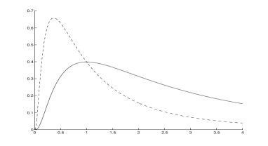
Figure 1: Density functions $\Lambda(0,1)$ (- - - -) and ${\cal N}_{+}(0,1)$ (——).

According to this approach, the normal distribution in $\mathbb{R}_{+}$ exhibits the same characteristics as the normal distribution in $\mathbb{R}$, the most relevant of which are summarized in the following properties. A complete proof of the following properties is presented in the appendix.

• Let be $X\sim{\cal N}_{+}(\mu,\sigma^{2})$, and constants $a\in\mathbb{R}_{+}$ and $b\in\mathbb{R}$. Then, the random variable $X^{*}=a\oplus(b\odot X)=a\cdot X^{b}$ is distributed as ${\cal N}_{+}(\ln a+b\mu,b^{2}\sigma^{2})$.

• Let be $X\sim{\cal N}_{+}(\mu,\sigma^{2})$ and $a\in\mathbb{R}_{+}$. Then, $f_{a\oplus X}^{+}(a\oplus x)=f_{X}^{+}(x)$,where $f_{X}^{+}$ and $f_{a\oplus X}^{+}$ represent the probability density functions of the random variables $X$ and $a\oplus X=a\cdot X$, respectively.

• If $X\sim{\cal N}_{+}(\mu,\sigma^{2})$, then $\mathrm{E}^{+}[X]=\mathrm{Med}^{+}[X]=\mathrm{Mode}^{+}[X]=e^{\mu}$.

• If $X\sim{\cal N}_{+}(\mu,\sigma^{2})$, then $\mathrm{Var}[X]=\sigma^{2}$.

Notice that Property 1 implies that the family ${\cal N}_{+}(\mu,\sigma^{2})$ is closed under the operations in $\mathbb{R}^{+}$ and Property 2 asserts the invariance under translations in $\mathbb{R}^{+}$.

The expected value, the median and the mode are elements of the support space $\mathbb{R}_{+}$, but the variance is only a numerical value which describes the dispersion of $X$. We are used to take the square root of $\sigma^{2}$ as a way to represent intervals centered at the mean and with radius equal to some standard deviations. To obtain such an interval centered at $\mathrm{E}[X]=e^{\mu}$ with length $2k\sigma$, take $(e^{\mu-k\sigma},e^{\mu+k\sigma})$ as $\mathrm{d}_{+}(e^{\mu-k\sigma},e^{\mu+k\sigma})=2k\sigma$. This kind of interval is used in practice (Ahrens, 1954) and predictive intervals in $\mathbb{R}_{+}$ taking exponential of predictive intervals computed from the log-transformed data under the hypothesis of normality are obtained. In Fig.2(a) we represent the interval $(e^{\mu-\sigma},e^{\mu+\sigma})$ for a ${\cal N}_{+}(\mu,\sigma^{2})$ density function with $\mu=0$ and $\sigma^{2}=1$. It can be shown that it is of minimum length, and it is also an isodensity interval thus, the distribution is symmetric around $e^{\mu}$. This symmetry might seem paradoxical, as one cannot see it in the shape of the density function. But still, it is symmetric within the linear vector space structure of $\mathbb{R}_{+}$, although certainly not within the Euclidean space structure of $\mathbb{R}_{+}$ as a subset of $\mathbb{R}$.

An important aspect of this approach is that consistent estimators and exact confidence intervals for the expected value are easy to obtain. We have only to take exponentials of those obtained from normal theory using log-transformed data, i.e. the coordinates with respect to the orthonormal basis. Thus, let be $x_{1},x_{2},\ldots,x_{n}$ a random sample and $y_{i}=\ln x_{i}$ for $i=1,2,\ldots,n$, then the optimal estimator for the mean of a normal in $\mathbb{R}_{+}$ population is the geometric mean $(x_{1}x_{2}\cdots x_{n})^{1/n}$ that equals to $e^{\bar{y}}$. An exact $(1-\alpha)100\%$ confidence interval for the mean is $(e^{{\bar{y}}-t_{\alpha/2}V/\sqrt{n}},e^{{\bar{y}}-t_{\alpha/2}V/\sqrt{n}})$ where $V$ denotes the logarithmic variance.

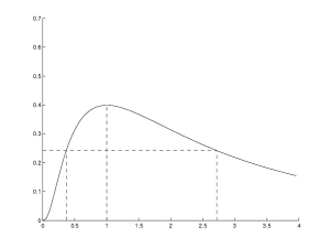
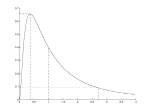
(a)	(b)

Figure 2: Interval $(e^{\mu-\sigma},e^{\mu+\sigma})$ in dashed line (a) ${\cal N}_{+}(\mu=0,\sigma^{2}=1)$, (b) $\Lambda(\mu=0,\sigma^{2}=1)$.

3.2 Normal on R+ vs lognormal

The lognormal distribution has long been recognized as a useful model in the evaluation of random phenomena whose distribution is positive and skew, and specially when dealing with measurements in which the random errors are multiplicative rather than additive. The history of this distribution starts in 1879, when Galton (1879) observed that the law of “frequency of errors” was incorrect in many groups of vital and social phenomena. This observation was based on Fechner’s law which, in its approximate and simplest form, is “sensation=log(stimulus)”. According to this law, an error of the same magnitude in excess or in deficiency (in the absolute sense) is not equally probable; therefore, he proposed the geometric mean as a measure of the most probable value instead of the arithmetic mean. This remark was followed by the memoir of McAlister (1879), where a mathematical investigation concluding with the lognormal distribution is performed. He proposed a practical and easy method for the treatment of a data set grouped around its geometric mean: “convert the observations into logarithms and treat the transformed data set as a series round its arithmetic mean”, and introduced a density function called the “law of frequency” which is the normal density function applied to the log-transformed variable i.e. density (8). In order to compute probabilities in given intervals, he introduced also the “law of facility”, nowadays known as the lognormal density function.

A unified treatment of the lognormal theory is presented by Aitchison and Brown (1957) and more recent developments are compiled by Crow and Shimizu (1988). A great number of authors use the lognormal model from an applied point of view. Their approach assumes $\mathbb{R}_{+}$ to be a subset of the real line with the usual Euclidean geometry. This is how everybody understands the sentence “an error of the same magnitude in excess or in deficiency” in the same way. One might ask oneself why there is much to say about the lognormal distribution if the data analysis can be referred to the intensively studied normal distribution by taking logarithms. One of the generally accepted reasons is that parameter estimates are biased if obtained from the inverse transformation.

Recall that a positive random variable $X$ is said to be lognormally distributed with two parameters $\mu$ and $\sigma^{2}$ if $Y=\ln X$ is normally distributed with mean $\mu$ and variance $\sigma^{2}$. We write $X\sim\Lambda(\mu,\sigma^{2})$ and its probability density function is

$$f_{X}(x)=\left\{\begin{array}[]{ll}\frac{1}{\sqrt{2\pi}\sigma x}\exp\left(-\frac{1}{2}\left(\frac{\ln x-\mu}{\sigma}\right)^{2}\right)&x>0,\\ 0&x\leq 0.\end{array}\right.$$ (9)

Comparing (9) with (8), we find some subtle differences. In fact, the expression of the lognormal density (9) includes a case for the zero and for the negative values of the random variable. This fact is paradoxical, because the lognormal model is completely restricted to $\mathbb{R}_{+}$. It is forced by the fact that $\mathbb{R}_{+}$ is considered as a subset of $\mathbb{R}$ with the same structure and, consequently, the variable is assumed to be a real random variable, hence the name “lognormal distribution in $\mathbb{R}$”. Another difference lies in the coefficient $1/x$, the Jacobian, which is necessary to work with real analysis in $\mathbb{R}$. More obvious differences are that (9) is not invariant under translations, that it is not symmetric around the mean, and that $\mathrm{E}[X]=e^{\mu+\frac{1}{2}\sigma^{2}}$, while $\mathrm{Med}[X]=e^{\mu}$, and both are different from the mode. The dashed line in Fig.1 illustrates the probability density function (9) for $\mu=0$ and $\sigma^{2}=1$. Observe that it differs from the density function (8) plotted in continuous line.

However, we can also find some coincidences between the two models. The median of a $\Lambda(\mu,\sigma^{2})$ model is equal to the median of a ${\cal N}_{+}(\mu,\sigma^{2})$ model. The same happens with any percentile and any value that involves the distribution function in its calculation. This property can be easily shown using measure theory, in particular using properties of integration with respect to the adequate measure. In fact, given a lognormal distributed variable $X$ with parameters $\mu$ and $\sigma^{2}$, the probability of any interval $(a,b)$ with $0<a<b$ is

$$P(a<X<b)=\int_{a}^{b}\frac{1}{\sqrt{2\pi}\sigma x}\exp\left(-\frac{1}{2}\left(\frac{\ln x-\mu}{\sigma}\right)^{2}\right)d\lambda(x).$$

The same probability could be computed using the normal in $\mathbb{R}_{+}$ model. Remember that in this case we work in the coordinates space, thus the probability of any interval $(a,b)$ is

$$P(a<X<b)=\int_{\ln a}^{\ln b}\frac{1}{\sqrt{2\pi}\sigma}\exp\left(-\frac{1}{2}\left(\frac{\ln x-\mu}{\sigma}\right)^{2}\right)d\lambda(\ln x).$$

Obviously the same result is obtained in both cases. Therefore we conclude that the lognormal and the normal in $\mathbb{R}_{+}$ are the same probability law over $\mathbb{R}_{+}$.

As we have made for the normal in $\mathbb{R}_{+}$ case, we could represent an interval centered at the mean and with radius equal to some standard deviations for the lognormal in $\mathbb{R}$. If we consider $\mathbb{R}_{+}$ as a subset of $\mathbb{R}$ with an Euclidean structure, these intervals are: $(\mathrm{E}[X]-k\mathrm{Stdev}[X],\mathrm{E}[X]+k\mathrm{Stdev}[X])$. But it has no sense, because the lower bound might take a negative value. For example, for $\mu=0$ and $\sigma^{2}=1$, the above interval with $k=1$ is $(-0.512,3.810)$. This is the reason why sometimes intervals $(e^{\mu-k\sigma},e^{\mu+k\sigma})$ are used, which are considered to be “non-optimal” because they are neither isodensity intervals, nor do they have minimum length. In Fig.2(b) we represent the interval $(e^{\mu-\sigma},e^{\mu+\sigma})$ for the $\Lambda(\mu,\sigma^{2})$ density function with $\mu=0$ and $\sigma^{2}=1$. It is clear that in the bounds of the interval the density function takes different values.

Consistent estimators and exact confidence intervals for the mean and the variance of a lognormal variable are difficult to compute. Early method of estimating are summarised in Aitchison and Brown (1957) and Crow and Shimizu (1988). Certainly we find in the literature and extensive number of procedures and discussions. It is not the objective of this paper to summarise all methods and to provide a complete set of formulas. But in general we could say that for the mean, the term $e^{\bar{y}}$ multiplied by a term expressed as an infinite serie or tabulated in a set of tables is obtained in most cases (Aitchison and Brown, 1957; Krige, 1981; Clark and Harper, 2000). For example, in Clark and Harper (2000) the Sichel’s optimal estimator for the mean of a lognormal population is used. This estimator is obtained as $e^{\bar{x}}\gamma$, where $\gamma$ is a bias correction factor depending on the variance and the size of the data set and tabulated in a set of tables. A similar bias correction factor is used to obtain confidence intervals on the population mean (Clark and Harper, 2000). Nevertheless, in practical situations, the geometric mean or $e^{\bar{y}}$ is used to represent the mean and in some cases also to represent the mode of a lognormal distributed variable (Herdan, 1960). But as adverted by Crow and Shimizu (1988) those affirmations cannot be justified using the lognormal theory. On the contrary, using the normal in $\mathbb{R}_{+}$ approach those affirmations are completely justified.

3.3 Example

The importance of using the normal in $\mathbb{R}_{+}$ instead of the lognormal in $\mathbb{R}$ can be best appreciated in practice.

In order to compare the classical lognormal estimators with those obtained by the normal in $\mathbb{R}_{+}$ approach, we have simulated 300 samples representing sizes of oil fields in thousands of barrels, a geological variable often lognormally modeled (Davis, 1986). Using the classical lognormal procedures and table A2 provided in Aitchison and Brown (1957) we obtain $161.96$ as an estimate for the mean. Afterwards and using tables 1,2 and 3 given in Krige (1981) we obtain $162.00$ and $(150.31,176.78)$ as an estimate and approximate $90\%$ confidence interval for the mean. Also, using tables 7, 8(b) and 8(e) provided in Clark and Harper (2000) we could apply the Sichel’s bias correction and we obtain $161.86$ and $(144.07,188.39)$ as the optimal estimator and confidence interval for the mean in the context of the lognormal approach.

Using the normal in $\mathbb{R}_{+}$ approach we easily obtain $145.04$ as the estimate for the mean and $(138.70,151.68)$ as the exact $90\%$ confidence interval for the mean. We have only to take exponentials of the mean and the $90\%$ confidence interval obtained from normal theory using log-transformed data. As can be observed, the differences from those obtained using the lognormal approach are important. With the normal in $\mathbb{R}_{+}$ a much more conservative result is obtained.

In order to compare graphically the normal in $\mathbb{R}_{+}$ and the lognormal approaches we can represent the histogram with the corresponding fitted densities. In Fig.3(a) and 3(b) the histogram with the fitted lognormal and normal in $\mathbb{R}_{+}$ densities are provided. Note that the intervals of the histogram are of equal length in both cases, as the absolute Euclidean distance is used in (a) and the relative distance in $\mathbb{R}_{+}$, $\mathrm{d}_{+}$, is used in (b) to compute them. Thus, (b) is a classical histogram but considering the structure defined in Section 2. Finally, in Fig.4 the histogram of the logtransformed data or equivalently of the coordinates with respect to the orthonormal basis with the fitted normal density is provided. This last figure is adequate using both methodologies but in this case we have chosen exactly the same intervals as in Fig.3(b). This is only possible using the normal in $\mathbb{R}_{+}$ approach because the intervals on the positive real line have the corresponding intervals in the space of coordinates.

The normal on $\mathbb{R}_{+}$ model and its properties has been recently applied in a spatial context and the results have seen compared with those obtained with the classical lognormal kriging approach (Tolosana-Delgado and Pawlowsky-Glahn, 2007). Using the proposed model and methodology, the problems of non-optimality, robustness and preservation of distribution disappear.

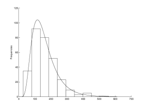
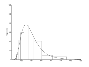
(a)	(b)

Figure 3: Simulated sample $n=300$. Histogram with (a) the fitted lognormal density and (b) with the fitted normal in $\mathbb{R}_{+}$ density.

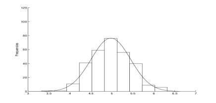
Figure 4: Simulated sample $n=300$. Histogram of the logtransformed sample with the fitted normal density.

4 The simplex

Compositional data are parts of some whole which give only relative information. Typical examples are parts per unit, percentages, ppm, and the like. Their sample space is the simplex, $\mathcal{S}^{D}=\{\mathbf{x}=(x_{1},x_{2},\ldots,x_{D})^{\prime}:x_{1}>0,x_{2}>0,\ldots,x_{D}>0;\;\sum_{i=1}^{D}x_{i}=\kappa\}$, where the prime stands for transpose and $\kappa$ is a constant (Aitchison, 1982). For vectors of proportions which do not sum to a constant, always a fill up value can be obtained.

The simplex $\mathcal{S}^{D}$ has a $(D-1)$-dimensional Euclidean space structure (Billheimer et. al., 2001; Pawlowsky and Egozcue, 2001) with the following operations. Let $\mathcal{C}(\cdot)$ denote the closure operation which normalises any vector $\mathbf{x}$ to a constant sum (Aitchison, 1982), and let be $\mathbf{x},\mathbf{x}^{*}\in\mathcal{S}^{D}$, and $\alpha\in\mathbb{R}$. Then, the inner sum, called perturbation, is defined as $\mathbf{x}\oplus{\mathbf{x}^{*}}={\cal C}\left(x_{1}x_{1}^{*},x_{2}x_{2}^{*},\ldots,x_{D}x_{D}^{*}\right)^{\prime}$; the outer product, called powering, is defined as $\alpha\odot\mathbf{x}=\mathcal{C}(x_{1}^{\alpha},x_{2}^{\alpha},\ldots,x_{D}^{\alpha})^{\prime}$; and the inner product is defined as

$$\langle\mathbf{x},\mathbf{x}^{*}\rangle_{a}=\frac{1}{D}\sum_{i<j}\ln\frac{x_{i}}{x_{j}}\ln\frac{x_{i}^{*}}{x_{j}^{*}}\ .$$ (10)

The associated squared distance is $\mathrm{d}_{a}^{2}(\mathbf{x},\mathbf{x}^{*})=(1/D)\sum_{i<j}(\ln({x_{i}}/{x_{j}})-\ln({x_{i}^{*}}/{x_{j}^{*}}))^{2}.$ This distance is relative and satisfies standard properties of a distance (Martín-Fernández et. al., 1998), i.e. $\mathrm{d}_{a}(\mathbf{x},\mathbf{x}^{*})=\mathrm{d}_{a}(\mathbf{a}\oplus\mathbf{x},\mathbf{a}\oplus\mathbf{x}^{*})$ and $\mathrm{d}_{a}(\alpha\odot\mathbf{x},\alpha\odot\mathbf{x}^{*})=\mid\alpha\mid\mathrm{d}_{a}(\mathbf{x},\mathbf{x}^{*})$. The geometry here defined is known as Aitchison geometry, and therefore the subindex $a$ is used.

The inner product (10) and its associated norm, $\|\mathbf{x}\|_{a}=\sqrt{\langle\mathbf{x},\mathbf{x}\rangle_{a}}$, ensure the existence of orthonormal basis $\{\mathbf{e}_{1},\mathbf{e}_{2},\ldots,\mathbf{e}_{D-1}\}$, which lead to a unique expression of a composition $\mathbf{x}$ as a linear combination,

$$\mathbf{x}=(\langle\mathbf{x},\mathbf{e}_{1}\rangle_{a}\odot\mathbf{e}_{1})\oplus(\langle\mathbf{x},\mathbf{e}_{2}\rangle_{a}\odot\mathbf{e}_{2})\oplus\ldots\oplus(\langle\mathbf{x},\mathbf{e}_{D-1}\rangle_{a}\odot\mathbf{e}_{D-1}).$$

Like in every inner product space, the orthonormal basis is not unique. It is not straightforward to determine which one is the most appropriate to solve a specific problem, but a promising strategy, based on binary partitions, has been developed by Egozcue and Pawlowsky (2005). Here, whenever a specific basis is needed, the basis given in Egozcue et. al. (2003) is used with respect to which the coordinates of any $\mathbf{x}\in\mathcal{S}^{D}$ are

$$y_{i}=\frac{1}{\sqrt{i(i+1)}}\ln\left(\frac{x_{1}x_{2}\cdots x_{i}}{x_{i+1}^{i}}\right)\ ,\qquad i=1,2,\ldots,D-1\;.$$ (11)

The coordinates in this particular basis are denoted $\mathrm{ilr}(\mathbf{x})$ to emphasise the similarity with the vector obtained applying the isometric log-ratio transformation to a composition $\mathbf{x}$, which is a transformation from $\mathcal{S}^{D}$ to $\mathbb{R}^{D-1}$ (Egozcue et. al., 2003). The important point is that, once an orthonormal basis has been chosen, all standard statistical methods can be applied to the coordinates and transferred to the simplex preserving their properties.

As stated in Section 2, the Lebesgue measure in the space of coordinates induces a measure in $\mathcal{S}^{D}$, denoted here as $\lambda_{a}$. This measure is absolutely continuous with respect to the Lebesgue measure on real space, and the relationship between them is $\left|{d\lambda_{a}}/{d\lambda}\right|=(\sqrt{D}\ x_{1}x_{2}\cdots x_{D})^{-1}.$

Following the notation in Section 2, all these definitions can be obtained by setting $E=\mathcal{S}^{D}$ and $d=D-1$.

For later use, the concept of subcomposition is required. For $C<D$, a $C$-part subcomposition, ${\mathbf{x}_{S}}$, from a $D$-part composition, $\mathbf{x}$, can be obtained as ${\mathbf{x}_{S}}=\mathcal{C}(\mathbf{S}\mathbf{x})$, where $\mathbf{S}$ is a $C\times D$ selection matrix with $C$ elements equal to 1 (one in each row and at most one in each column) and the remaining elements equal to 0 (Aitchison, 1986). A subcomposition can be regarded as a composition in a simplex with fewer parts, and thus as a space of lower dimension.

4.1 Some basic statistical concepts in the simplex

A random composition $\mathbf{X}$ is a random vector with $\mathcal{S}^{D}$ as domain. In the literature laws of probability over $\mathcal{S}^{D}$ can be found, defined using the standard methodology, i.e. using the Lebesgue measure. Consequently, the probabilities or any moment are computed using the classical definition. But some usual elements appear to be of little use when working with real situations. One typical example is the expected value which appears as not representative as a measure of location. As an alternative, the geometric interpretation of the expected value has been used to define the centre, $\mathrm{cen}[\mathbf{X}]$, of a random composition as that composition which minimises the expression $\mathrm{E}[\mathrm{d}_{a}^{2}(\mathbf{X},\mathrm{cen}[\mathbf{X}])]$ (Aitchison, 1997; Pawlowsky and Egozcue, 2001). The result is $\mathrm{cen}[\mathbf{X}]=\mathcal{C}(\exp(\mathrm{E}[\ln\mathbf{X}]))$, which can be rewritten as (Egozcue et. al., 2003) $\mathrm{cen}[\mathbf{X}]=\mathrm{ilr}^{-1}(\mathrm{E}[\mathrm{ilr}(\mathbf{X})])$, or, in general terms, as

$$\mathrm{cen}[\mathbf{X}]=h^{-1}\left(\mathrm{E}\left[h(\mathbf{X})\right]\right).$$ (12)

Observe that the centre of a random composition is equal to the expectation in $\mathcal{S}^{D}$ defined in Section 2. This is an important result because if a law of probability on $\mathcal{S}^{D}$ is defined using the classical approach, this equality does not hold.

As already mentioned, traditionally the simplex has been considered as a subset of real space and, consequently, the laws of probability have been defined using the standard approach. This is the case for families of distributions like the Dirichlet, the additive logistic normal (Aitchison, 1982), the additive logistic skew-normal (Mateu-Figueras et.at., 2005), or those defined using the Box-Cox family of transformations (Barceló-Vidal, 1996). Except for the Dirichlet, these laws of probability are defined using transformations from the simplex to real space. Two of these transformations will appear later in this paper, the additive log-ratio $(\mathrm{alr})$ and the centred log-ratio $(\mathrm{clr})$,

$$\mathrm{alr}(\mathbf{x})=\left(\ln\left(\frac{x_{1}}{x_{D}}\right),\ldots,\ln\left(\frac{x_{D-1}}{x_{D}}\right)\right)^{\prime},\mathrm{clr}(\mathbf{x})=\left(\ln\left(\frac{x_{1}}{g(\mathbf{x})}\right),\ldots,\ln\left(\frac{x_{D}}{g(\mathbf{x})}\right)\right)^{\prime},$$

where $g(\mathbf{x})$ is the geometric mean of composition $\mathbf{x}$. The relationship between the $\mathrm{alr}$ and the $\mathrm{clr}$ transformations is provided by Aitchison (1986) (p.92). The relationships between the $\mathrm{alr}$, $\mathrm{clr}$ and $\mathrm{ilr}$ transformations are provided by Egozcue et. al. (2003).

4.2 The normal distribution on SD

Using the algebraic-geometric structure and the measure $\lambda_{a}$ on $\mathcal{S}^{D}$, the normal distribution on $\mathcal{S}^{D}$ is defined through the density function of generic orthonormal coordinates $h(\mathbf{X})$ (Mateu-Figueras, 2003). The same strategy is used in Mateu-Figueras and Pawlowsky-Glahn (2007) to define the skew-normal in $\mathcal{S}^{D}$ law.

Definition 2. Let be $(\Omega,{\cal F},p)$ a probability space. A random composition $\mathbf{X}:\Omega\longrightarrow\mathcal{S}^{D}$ is said to have a regular normal on $\mathcal{S}^{D}$ distribution, with parameters $\mu$ and $\mathbf{\Sigma}$, if its density function is

$$f_{\mathbf{X}}^{\mathcal{S}}(\mathbf{x})=(2\pi)^{-(D-1)/2}|\mathbf{\Sigma}|^{-1/2}\exp\left(-{\frac{1}{2}}\left(h(\mathbf{x})-\mbox{\boldmath$\mu$}\right)^{\prime}\mathbf{\Sigma}^{-1}\left(h(\mathbf{x})-\mbox{\boldmath$\mu$}\right)\right),$$ (13)

where $h(.)$ stands for the generic orthonormal coordinates.

The notation $\mathbf{X}\sim\mathcal{N}_{\mathcal{S}}^{D}(\mbox{\boldmath$\mu$},\mathbf{\Sigma},\mbox{\boldmath$\alpha$})$ is used. The subscript $\mathcal{S}$ indicates that it is a model on the simplex and the superscript $D$ indicates the number of parts of the composition. Fig.5 shows the isodensity curves of two normal densities on $\mathcal{S}^{3}$ taking the particular basis given by Egozcue et. al. (2003) and using a ternary diagram as a convenient and simple way for representing 3-part compositions (see Aitchison, 1986, p.6).

The density (13) is the usual normal density applied to coordinates $h(\mathbf{x})$ as implied by (4) and it is a density in $\mathcal{S}^{D}$ with respect to the $\lambda_{a}$ measure.

The principal properties of this model follow. A complete proof of each property can be found in the appendix. The proofs are straightforward for a reader familiar with compositional data analysis.

• Let be $\mathbf{X}\sim\mathcal{N}_{\mathcal{S}}^{D}(\mbox{\boldmath$\mu$},\mathbf{\Sigma})$, $\mathbf{a}\in\mathcal{S}^{D}$ and $b\in\mathbb{R}$. Then, the $D$-part random composition $\mathbf{X}^{*}=\mathbf{a}\oplus(b\odot\mathbf{x})$ has a $\mathcal{N}_{\mathcal{S}}^{D}(h(\mathbf{a})+b\mbox{\boldmath$\mu$},b^{2}\mathbf{\Sigma})$ distribution.

• Let be $\mathbf{X}\sim\mathcal{N}_{\mathcal{S}}^{D}(\mbox{\boldmath$\mu$},\mathbf{\Sigma})$ and $\mathbf{a}\in\mathcal{S}^{D}$. Then $f_{\mathbf{a}\oplus\mathbf{X}}^{\mathcal{S}}(\mathbf{a}\oplus\mathbf{x})=f_{\mathbf{X}}^{\mathcal{S}}(\mathbf{x})$, where $f_{\mathbf{X}}^{\mathcal{S}}$ and $f_{\mathbf{a}\oplus\mathbf{X}}^{\mathcal{S}}$ represent the density functions of the random compositions $\mathbf{X}$ and $\mathbf{a}\oplus\mathbf{X}$, respectively.

• Let be $\mathbf{X}\sim\mathcal{SN}_{\mathcal{S}}^{D}(\mbox{\boldmath$\mu$},\mathbf{\Sigma})$ and $\mathbf{X}_{P}={\mathbf{PX}}$, the random composition $\mathbf{X}$ with the parts reordered by a permutation matrix ${\mathbf{P}}$. Then $\mathbf{X}_{P}\sim\mathcal{N}_{\mathcal{S}}^{D}(\mbox{\boldmath$\mu$}_{P},\mathbf{\Sigma}_{P})$ with $\mbox{\boldmath$\mu$}_{P}={\mathbf{U^{\prime}PU}}\mbox{\boldmath$\mu$}$, $\mathbf{\Sigma}_{P}=({\mathbf{U^{\prime}PU}})\mathbf{\Sigma}({\mathbf{U^{\prime}P^{\prime}U}})$, where ${\mathbf{U}}$ is a $D\times(D-1)$ matrix with the clr transformation of a generic orthonormal basis of $\mathcal{S}^{D}$ as columns.

• Let be $\mathbf{X}\sim\mathcal{N}_{\mathcal{S}}^{D}(\mbox{\boldmath$\mu$},\mathbf{\Sigma})$ and ${\mathbf{X}_{S}}=\mathcal{C}({\mathbf{S}}\mathbf{X})$, the $C$-part random subcomposition obtained from the $C\times D$ selection matrix ${\mathbf{S}}$. Then ${\mathbf{X}_{S}}\sim\mathcal{N}_{\mathcal{S}}^{C}(\mbox{\boldmath$\mu$}_{S},\mathbf{\Sigma}_{S})$, with $\mbox{\boldmath$\mu$}_{S}={{\mathbf{U}^{*}}}^{\prime}{\mathbf{SU}}\mbox{\boldmath$\mu$}$,$\mathbf{\Sigma}_{S}=({\mathbf{U}^{*}}^{\prime}{\mathbf{SU}})\mathbf{\Sigma}({\mathbf{U^{\prime}S^{\prime}}{\mathbf{U}^{*}}})$, where ${\mathbf{U}}$ is a $D\times(D-1)$ matrix with the $\mathrm{clr}$ transformation of a generic orthonormal basis of $\mathcal{S}^{D}$ as columns and ${\mathbf{U}}^{*}$ is a $C\times(C-1)$ matrix with the $\mathrm{clr}$ transformation of a generic orthonormal basis of $\mathcal{S}^{C}$ as columns.

• Let be $\mathbf{X}\sim\mathcal{N}_{\mathcal{S}}^{D}(\mbox{\boldmath$\mu$},\mathbf{\Sigma})$. Then, the expected value in $\mathcal{S}^{D}$ is

  $$\mathrm{E}_{a}[\mathbf{X}]=(\mu_{1}\odot\mathbf{e}_{1})\oplus(\mu_{2}\odot\mathbf{e}_{2})\oplus\ldots\oplus(\mu_{D-1}\odot\mathbf{e}_{D-1}).$$ (14)

• Let be $\mathbf{X}\sim\mathcal{N}_{\mathcal{S}}^{D}(\mbox{\boldmath$\mu$},\mathbf{\Sigma})$. The metric variance of $\mathbf{X}$ is $\mathrm{Var}[\mathbf{X}]=\hbox{trace}\left(\mathbf{\Sigma}\right)$.

From Property 5 we conclude that the normal on $\mathcal{S}^{D}$ law is closed under perturbation and powering. From Property 6 we see that it is also invariant under perturbation. This has important consequences, because when working with compositional data the centring operation (Martín-Fernández et. al., 1999), a perturbation using the inverse of the centre of the data set, is often applied in practice to better visualise and interpret the pattern of variability (von Eynatten et.al., 2002).

Notice that Properties 7 and 8 show that the normal on $\mathcal{S}^{D}$ family is closed under permutation and subcompositions.

Given a compositional data set the estimates of parameters $\mu$ and $\mathbf{\Sigma}$ can be computed applying the maximum likelihood procedure to the coordinates of the data set. The estimated values $\hat{\mbox{\boldmath$\mu$}}$ and $\widehat{\mathbf{\Sigma}}$ allow us to compute the estimates of the expected value and metric variance of random composition $\mathbf{X}$, as $\widehat{\mathrm{E}_{a}[\mathbf{X}]}=(\hat{\mu}_{1}\odot\mathbf{e}_{1})\oplus\cdots\oplus(\hat{\mu}_{D-1}\odot\mathbf{e}_{D-1})$ and $\widehat{\mathrm{Var}[\mathbf{X}]}=\hbox{trace}\left(\widehat{\mathbf{\Sigma}}\right)$.

To validate the distributional assumption of normality on $\mathcal{S}^{D}$, some goodness-of-fit tests of the multivariate normal distribution have to be applied to the coordinates of the sample data set. There is a large battery of possible tests but as suggested by Aitchison (1986) we could start testing the normality of each marginal using empirical distribution function tests. Unfortunately, the univariate normality of each component is a necessary but not sufficient condition for the normality of the whole vector. Also, these univariate tests depend on the orthonormal basis chosen. This difficulty does not depend on the proposed methodology, as the same problem appears when working with laws of probability defined using transformations and the Lebesgue measure in $\mathcal{S}^{D}$ (Aitchison et.al., 2003). The multivariate normal model can also be validated considering the Mahalanobis distance $(h(\mathbf{X})-\hat{\mbox{\boldmath$\mu$}})^{\prime}\widehat{\mathbf{\Sigma}}^{-1}(h(\mathbf{X})-\hat{\mbox{\boldmath$\mu$}})$ which is sampled from a $\chi^{2}_{D-1}$-distribution if the fitted model is appropriate. In this case, the dependence on the chosen orthonormal basis disappears. Here, the use of empirical distribution function tests is also suggested (Aitchison, 1986).

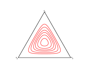
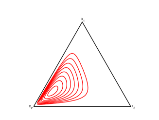
(a)	(b)

Figure 5: Isodensity plots of two $\mathcal{N}_{\mathcal{S}}^{3}(\mbox{\boldmath$\mu$},\mathbf{\Sigma})$ with (a) $\mbox{\boldmath$\mu$}=(0,0)$, (b) $\mbox{\boldmath$\mu$}=(-1,1)$ and $\mathbf{\Sigma}=Id$.

4.3 The normal on SD vs the additive logistic normal

The classical approach is used by Aitchison (1982) to define the additive logistic normal law on the simplex. The strategy is standard: transform the random composition from the simplex to the real space, define the density function of the transformed vector and finally go back to the simplex using the theorem of the change of variable. The result is a density function for the initial random composition with respect to the Lebesgue measure. Thus, a random composition is said to have an additive logistic normal distribution ($\mathrm{aln}$) when the additive log-ratio transformed vector has a normal distribution. Note that this definition does not explicitly state that the theorem of the change of variable has to be used. But this is the principal difference between this approach, based on working with transformations, with the new approach, based on working with coordinates.

The $\mathrm{aln}$ model was initially defined using the additive log-ratio transformation. Using the matrix relationship among the log-ratio transformations (Egozcue et. al., 2003) we can easily obtain the density function in terms of the isometric log-ratio transformation. Thus we can define the logistic normal distribution with parameters $\mu$ and $\mathbf{\Sigma}$, with density function:

$$f_{\mathbf{X}}(\mathbf{x})=\frac{(2\pi)^{-(D-1)/2}\mid\mathbf{\Sigma}\mid^{-1/2}}{\sqrt{D}x_{1}x_{2}\cdots x_{D}}\exp\left(-{\frac{1}{2}}\left(\mathrm{ilr}(\mathbf{x})-\mbox{\boldmath$\mu$}\right)^{\prime}\mathbf{\Sigma}^{-1}\left(\mathrm{ilr}(\mathbf{x})-\mbox{\boldmath$\mu$}\right)\right).$$ (15)

To easily compare both approaches we will use the normal model on the simplex taking the basis given in Egozcue et. al. (2003) and consequently the $\mathrm{ilr}$ vector stated in (11). Nevertheless, we could consider any orthonormal basis as we can obtain vector $\mathrm{ilr}(\mathbf{x})$ from $h(\mathbf{x})$ and the corresponding change of basis matrix. If we compare the expression of the densities (13) and (15), the only difference is the term $(\sqrt{D}x_{1}x_{2}\cdots x_{D})^{-1}$, the jacobian of the isometric log-ratio transformation that reflects the change of the measure on $\mathcal{S}^{D}$. The influence of this term can be observed in the isodensity curves in Fig.6. These curves can be directly compared with the curves in Fig.5. The differences are obvious, in particular the trimodality in Fig.6(a). This behaviour is not exclusive of the logistic normal model, we find also bimodality with Beta or Dirichlet densities when their parameters tend to 0 and when the Lebesgue measure is considered. In Fig.6(b) we observe a unique mode, nevertheless its position and the shape of the curves are not the same as in Fig.5(b), the corresponding normal on $\mathcal{S}^{3}$.

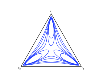
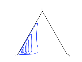
(a)	(b)

Figure 6: Isodensity plots of two logistic normal models with (a) $\mbox{\boldmath$\mu$}=(0,0)$, (b) $\mbox{\boldmath$\mu$}=(-1,1)$ and $\mathbf{\Sigma}=Id$.

Another essential difference between the two models are the moments of any order. We know that the expression of the density function plays a fundamental role when any moment is computed. The density (15) is a classical density, consequently we compute any moment using the standard definition. Obviously the results are not the same as in the normal on $\mathcal{S}^{D}$ case. For example, the expected value of an $\mathrm{aln}$ model exists, but numerical procedures have to be applied (see Aitchison, 1986, p.116) to find it and the result is not the same as in Property 9.

Also, some coincidences can be found. The closure under perturbation, powering, permutation and subcompositions of the logistic normal model is proved by Aitchison (1986), the same as those stated in Properties 5,7 and 8 for the normal on $\mathcal{S}^{D}$ model. Nevertheless the logistic normal class is not invariant under perturbation, that is, $f_{\mathrm{a}\oplus\mathbf{X}}(\mathrm{a}\oplus\mathbf{x})\neq f_{\mathbf{X}}(\mathbf{x})$.

Another coincidence is that the two models assign the same probability to the events and we can say that both models are equivalent on $\mathcal{S}^{D}$. In fact, given a logistic normal distributed random composition $\mathbf{X}$ with parameters $\mu$ and $\mathbf{\Sigma}$, the probability of any event $A\subseteq\mathcal{S}^{D}$ is

$$P(A)=\int_{A}\frac{(\sqrt{D}x_{1}x_{2}\cdots x_{D})^{-1}}{\mid\mathbf{\Sigma}\mid^{1/2}(2\pi)^{(D-1)/2}}\exp\left(-{\frac{1}{2}}\left(\mathrm{ilr}(\mathbf{x})-\mbox{\boldmath$\mu$}\right)^{\prime}\mathbf{\Sigma}^{-1}\left(\mathrm{ilr}(\mathbf{x})-\mbox{\boldmath$\mu$}\right)\right)d\lambda(\mathbf{x}),$$ (16)

where now the vector $\mathrm{ilr}(\mathbf{x})$ denotes the isometric log-ratio transformation of vector $\mathbf{x}$. The same probability using the normal on $\mathcal{S}^{D}$ model is

$$P(A)=\int_{\mathrm{ilr}(A)}\frac{1}{\mid\mathbf{\Sigma}\mid^{1/2}(2\pi)^{(D-1)/2}}\exp\left(-{\frac{1}{2}}\left(\mathbf{v}-\mbox{\boldmath$\mu$}\right)^{\prime}\mathbf{\Sigma}^{-1}\left(\mathbf{v}-\mbox{\boldmath$\mu$}\right)\right)d\lambda(\mathbf{v}),$$ (17)

with $\mathrm{ilr}(A)$ giving now the representation of event $A$ in coordinates with respect to the particular orthonormal basis given by Egozcue et. al. (2003). At this point it is important to correctly interpret the vector $\mathrm{ilr}(\mathbf{x})$ as the isometric log-ratio transformed vector or as the vector of coordinates. Therefore, to avoid possible confusions, we denote by $\mathbf{v}$ the vector of coordinates in expression (17). Certainly, the two vectors are numerically identical, but here the meaning is important.

Both expressions (16) and (17) are standard integrals of a real valued function. Thus, we can apply a change of variable in (17), taking $\mathbf{v}=\mathrm{ilr}(\mathbf{x})$ whose jacobian is $(\sqrt{D}x_{1}x_{2}\cdots x_{D})^{-1}$, and the equality

$$P(A)=\int_{A}\frac{(\sqrt{D}x_{1}x_{2}\cdots x_{D})^{-1}}{\mid\mathbf{\Sigma}\mid^{1/2}(2\pi)^{(D-1)/2}}\exp\left(-{\frac{1}{2}}\left(\mathrm{ilr}(\mathbf{x})-\mbox{\boldmath$\mu$}\right)^{\prime}\mathbf{\Sigma}^{-1}\left(\mathrm{ilr}(\mathbf{x})-\mbox{\boldmath$\mu$}\right)\right)d\lambda(\mathbf{x})$$

is obtained. This equality agrees with (16) given that $\mathrm{ilr}^{-1}(\mathrm{ilr}(A))=A$. Remember that an isometric log-ratio transformed element is equal to its coordinates with respect to the orthonormal basis given by Egozcue et. al. (2003). Then, the $\mathrm{ilr}^{-1}$ transformation gives the original element on the simplex. Therefore we conclude that the additive logistic normal law and the normal on $\mathcal{S}^{D}$ law are the same probability law over the simplex.

Concerning estimation and goodness-of-fit testing, we will obtain exactly the same results using both models. Remember that in the normal in $\mathcal{S}^{D}$ case we work with the $\mathrm{ilr}$ coordinates whereas in the logistic normal case we work with the $\mathrm{ilr}$ transformed vector.

In summary, the essential differences between both approaches are the shape of the probability density function, in some cases leading to multimodality for the standard approach; the moments which characterise the density, particularly important in practice for the expected value and the variance; and invariance under perturbation.

4.4 Example

To illustrate the differences between using a density with respect to the Lebesgue measure $\lambda$ or a density with respect to the measure $\lambda_{a}$ in $\mathcal{S}^{D}$, the Skye lavas data (Thompson et.al., 1972) will be used. It contains chemical compositions of 23 basalt specimens from the Isle of Skye in the form of percentages of 10 major oxides. This data set is used in Aitchison (1982) to discuss the adequacy of some parametric models and no significant indication of non-normality is obtained for the $\mathrm{alr}$ transformed data set. Due to the matrix relationship between the $\mathrm{alr}$ and $\mathrm{ilr}$ transformations, we can easily conclude no significant departure from normality for the $\mathrm{ilr}$ transformed data set.

Our objective in this section is to compare graphically the logistic normal and the normal on the simplex. Thus, in order to provide some useful figures a 3-part compositional data set is preferred. For this reason we take $\mathbf{X}$ as the popular AFM subcomposition (A: $Na_{2}O+K_{2}O$, F: $Fe_{2}O_{3}$ and M:$MgO$) from the Skye lavas data set. The resulting data can be found in Aitchison (1986) or in Thompson et.al. (1972). As the first component is obtained amalgamating two original parts, we cannot guarantee the adequacy of the logistic normal and the normal in $\mathcal{S}^{3}$ models. Following the suggestions by Aitchison (1986) we could test the goodness-of-fit of the model applying a battery of 12 tests, based on the Anderson-Darling, Cramér-von Mises and Watson statistics, to the coordinates of the sample data set. In particular, the tests are applied to the marginal distributions, to the bivariate angle distribution and to the radius. Taking a 1 per cent significance level only one of the marginal tests gives evidence of any departure from normality.

The fit of a normal model on $\mathcal{S}^{3}$ and of a logistic normal model (using the $\mathrm{ilr}$ transformation) gives, as noted in the previous section, exactly the same estimates of the parameters for both models:

$$\hat{\mbox{\boldmath$\mu$}}=(0.555,0.639)^{\prime},\qquad\mathbf{\hat{\Sigma}}=\left(\begin{array}[]{cc}0.126&-0.229\\ -0.229&0.456\\ \end{array}\right).$$

Here, the orthonormal basis given by Egozcue et. al. (2003) has been used, and consequently the $\mathrm{ilr}$ vector stated in (11).

The fit of the logistic normal and normal in $\mathcal{S}^{3}$ models are represented in dashed line in Fig.7(a) and 7(b) respectively. The two fitted models are quite similar.

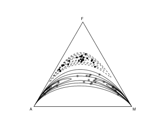
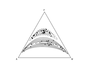
(a)	(b)

Figure 7: Skye lavas data $(\bullet)$ and linearly transformed data $(\ast)$ with isodensity curves of the fitted (a) logistic normal model and (b) normal on $\mathcal{S}^{3}$.

As both models follow Property 5, i.e. the families are closed under perturbation and powering, the transformation $\mathbf{a}\oplus(b\odot\mathbf{X})$ is applied to the data, with $\mathbf{a}=g(\mathbf{X})^{-1}$ and $b=\sqrt{3}$. This is a linear transformation in $\mathcal{S}^{3}$ and has been chosen only for illustration purposes. Note that the geometric mean of our resulting data set is the center of the simplex, composition $(1/3,1/3,1/3)$, because we first modify the variability applying the power operation but then we center our data. It is equivalent to translate the transformed data set, or the coordinates with respect to an orthonormal basis, to the origin of coordinates in the real space. For both resulting models the estimates of the parameters follow the equations stated in Property 5 i.e.

$$\hat{\mbox{\boldmath$\mu$}}=(0.000,0.000)^{\prime},\qquad\mathbf{\hat{\Sigma}}=\left(\begin{array}[]{cc}0.377&-0.688\\ -0.688&1.369\\ \end{array}\right).$$

In Fig.7(a) and 7(b) the logistic normal and the normal in $\mathcal{S}^{3}$ fitted models are represented in continuous line. As can be observed, the same linear transformation leads to a better visualisation of the normal on $\mathcal{S}^{3}$ fitted model, but in the logistic normal case a completely different model, with two modes, is obtained. In other words, perturbation and powering, which should only move the centre of the density and modify the variability, can generate arbitrary modes, an undesirable property. In Fig.8 we represent the corresponding normal densities fitted to the $\mathrm{ilr}$ coordinates or equivalently to the $\mathrm{ilr}$ transformed data set, because the same graphic is obtained using both methodologies. It is clear that the linear transformation only increase the variability and translate our data set to the origin of coordinates.

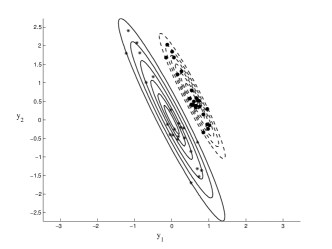
Figure 8: $\mathrm{ilr}$ coordinates of the Skye lavas data set and the corresponding fitted normal models to the original data (dashed line) and to the linear transformed data (continuous line).

5 Conclusions

A particular Euclidean vector space structure of the positive real line and of the simplex, together with the associated measure, allow us to define parametric models with desirable properties. Normal models on $\mathbb{R}_{+}$ and on $\mathcal{S}^{D}$ have been defined through their densities over the coordinates with respect to an orthonormal basis and their main algebraic properties have been studied. From a probabilistic point of view, those laws of probability are identical to the lognormal and to the additive logistic normal distribution defined using the Lebesgue measure and the standard methodology based on transformations. Nevertheless, some differences are obtained in the moments and in the shape of the density function. In particular, the expected value differs from what would be obtained with the lognormal and with the additive logistic normal distributions, something important when they are used to characterise real data using a probabilistic model.

APPENDIX

This appendix contains the proofs of properties contained in Sections 3.1 and 4.2. The construction of these proofs is done using the expected value, the covariance matrix, the linear transformation property of the multivariate normal distribution and some matrix relationships among vectors of coordinates and among log-ratio transformations.

Proof of Property 1. The coordinates of the random variable $X^{*}$ are obtained from the coordinates of the variable $X$ as $\ln(X^{*})=\ln(a)+b\ln(X)$. The density function of $\ln(X)$ is the classical normal density in the real line; thus, the linear transformation property can be used to obtain the density function of the $\ln(X^{*})$ random variable. Therefore, $X^{*}\sim{\cal N}_{+}(\ln a+b\mu,b^{2}\sigma^{2})$.

Proof of Property 2. From Property 1 we know that $a\oplus X=a\cdot X\sim{\cal N}_{+}(\ln a+\mu,\sigma^{2})$. From (8) we get

$$f^{+}_{a\oplus X}(a\oplus x)=\frac{1}{\sqrt{2\pi}\sigma}\exp\left(-\frac{1}{2}\frac{(\ln(ax)-(\ln a+\mu))^{2}}{\sigma^{2}}\right)=f^{+}_{X}(x).$$

Proof of Property 3. From (6) we known that $\mathrm{E}^{E}[X]=\exp((\mathrm{E}[\ln X])$, and from (8) we known that the density function of $\ln X$ is the normal distribution, thus $\mathrm{E}^{E}[X]=\exp(\mu)$. The same result is obtained for the median and the mode as the normal distribution is symmetric around its expected value $\mu$.

Proof of Property 4. From (7) we know that the variance can be understood as the expected value of the squared distance around its expected value, i.e. $\mathrm{Var}[X]=\\ \mathrm{E}[\mathrm{d}_{+}^{2}(X,\mathrm{E}^{+}[X])]$. Working on coordinates and using the density function of $\ln X$ we obtain $\mathrm{Var}[X]=\mathrm{E}[\mathrm{d}^{2}(\ln{X},\mathrm{E}[\ln{X}])]=\mathrm{Var}[\ln{X}]=\sigma^{2}$.

Proof of Property 5. The orthonormal coordinates of the random composition $\mathbf{X}^{*}$ are obtained from the orthonormal coordinates of the composition $\mathbf{X}$ via $h(\mathbf{X}^{*})=h(\mathbf{a})+bh(\mathbf{X})$. The density function of $h(\mathbf{X})$ random vector is the classical normal density in real space; thus, the linear transformation property can be used to obtain the density function of the $h(\mathbf{X}^{*})$ random vector. Therefore, $\mathbf{X}^{*}\sim\mathcal{N}_{\mathcal{S}}^{D}(h(\mathbf{a})+b\mbox{\boldmath$\mu$},b^{2}\mathbf{\Sigma},\mbox{\boldmath$\alpha$})$.

Proof of Property 6. Using Property 5, $\mathbf{a}\oplus\mathbf{X}\sim\mathcal{N}_{\mathcal{S}}^{D}(h(\mathbf{a})+\mbox{\boldmath$\mu$},\mathbf{\Sigma},\mbox{\boldmath$\alpha$})$. We known that $h(\mathbf{a}\oplus\mathbf{x})=h(\mathbf{a})+h(\mathbf{x})$, therefore,

$$f_{\mathbf{a}\oplus\mathbf{X}}(\mathbf{a}\oplus\mathbf{x}) =(2\pi)^{-(D-1)/2}\mid\mathbf{\Sigma}\mid^{-1/2}$$

$$\ \times\exp\left[-{\frac{1}{2}}\left(h(\mathbf{a}\oplus\mathbf{x})-(h(\mathbf{a})+\mbox{\boldmath$\mu$})\right)^{\prime}\mathbf{\Sigma}^{-1}\left(h(\mathbf{a}\oplus\mathbf{x})-(h(\mathbf{a})+\mbox{\boldmath$\mu$})\right)\right]=$$

$$=(2\pi)^{-(D-1)/2}\mid\mathbf{\Sigma}\mid^{-1/2}\exp\left[-{\frac{1}{2}}\left(h(\mathbf{x})-\mbox{\boldmath$\mu$}\right)^{\prime}\mathbf{\Sigma}^{-1}\left(h(\mathbf{x})-\mbox{\boldmath$\mu$}\right)\right]=f_{\mathbf{X}}(\mathbf{x}).$$

Proof of Property 7. For the centered log-ratio transformed vectors it is straightforward to see that $\mathrm{clr}(\mathbf{X}_{P})={\mathbf{P}}\mathrm{clr}(\mathbf{X})$ (Aitchison, 1986, p. 94). Using the matrix relationship between the centered and the isometric log-ratio vectors (Egozcue et. al., 2003) we conclude that $h(\mathbf{X}_{P})=({\mathbf{U^{\prime}PU}})h(\mathbf{X})$. Given the density of the $h(\mathbf{X})$ random vector, and applying the linear transformation property of the normal distribution in real space, a $\mathcal{N}_{\mathcal{S}}^{D}(\mbox{\boldmath$\mu$}_{P},\mathbf{\Sigma}_{P},\mbox{\boldmath$\alpha$}_{P})$ distribution is obtained for the random composition $\mathbf{X}_{P}$.

Proof of Property 8. (Aitchison, 1986, p. 119) gives the matrix relationship between $\mathrm{alr}(\mathbf{X}_{S})$ and $\mathrm{alr}(\mathbf{X})$. Using the matrix relationships between the additive, centered and isometric log-ratio vectors (Egozcue et. al., 2003), we conclude that $h(\mathbf{X}_{S})=({\mathbf{U}^{*}}^{\prime}{\mathbf{SU}})h(\mathbf{X})$. Given the density of the $h(\mathbf{X})$ vector, and applying the linear transformation property of the normal distribution in real space, the density of the $h(\mathbf{X}_{S})$ vector is obtained as that of the $\mathcal{N}_{\mathcal{S}}^{C}(\mbox{\boldmath$\mu$}_{S},\mathbf{\Sigma}_{S},\mbox{\boldmath$\alpha$}_{S})$ distribution.

Proof of Property 9. From (6) we known that $\mathrm{E}_{a}[\mathbf{X}]=h^{-1}(\mathrm{E}[h(\mathbf{X})])$, and from Definition 2 we know that the density function of $h(\mathbf{X})$ is the multivariate normal distribution; thus $\mathrm{E}[h(\mathbf{X})]=\mbox{\boldmath$\mu$}$. Finally, the composition $\mathrm{E}_{a}[\mathbf{X}]$ is obtained applying $h^{-1}$ or by the representation of this element in the basis $(\mu_{1}\odot\mathbf{e}_{1})\oplus(\mu_{2}\odot\mathbf{e}_{2})\oplus\ldots\oplus(\mu_{D-1}\odot\mathbf{e}_{D-1})$.

Proof of Property 10. From (7) we know that the variance can be understood as the expected value of the squared distance around its expected value, i.e. $\mathrm{Var}[\mathbf{X}]=\mathrm{E}[d_{a}^{2}(\mathbf{X},\mathrm{E}_{a}[\mathbf{X}])]$. Working on coordinates and using the density function of $h(\mathbf{X})$ we obtain $\mathrm{Var}[\mathbf{X}]=\mathrm{trace}(\mathbf{\Sigma})$.

References

- Ahrens (1954) Ahrens, L. (1954). The lognormal distribution of the elements.. Geochimica et Cosmochimica Acta,5, 49-73.
- Aitchison (1982) Aitchison, J. (1982). The statistical analysis of compositional data (with discussion). Journal of the Royal Statistical Society, Series B, 44(2), 139-177.
- Aitchison (1986) Aitchison, J. (1986). The Statistical Analysis of Compositional Data. Monographs on Statistics and Applied Probability. Chapman & Hall Ltd., London (UK). (Reprinted in 2003 with additional material by The Blackburn Press). 416 p.
- Aitchison (1997) Aitchison, J. (1997). The one-hour course in compositional data analysis or compositional data analysis is simple. In: Proceedings of IAMG’97, the third annual conference of the International Association for Mathematical Geology (ed: V. Pawlowsky-Glahn), vol 1, 3-35. International Center for Numerical Methods in Engineering (CIMNE), Barcelona (E).
- Aitchison and Brown (1957) Aitchison, J. and Brown, J.A.C. (1957). The lognormal distribution. Cambridge University Press. Cambridge (UK).
- Aitchison et.al. (2003) Aitchison, J., Mateu-Figueras, G. and Ng, K. (2003). Characterization of distributional forms for compositional data and associated distributional tests. Mathematical Geology,35(6), 667-680.
- Barceló-Vidal (1996) Barceló-Vidal, C. (1996). Mixturas de Datos Composicionales. Ph. D. Thesis, Universitat Politècnica de Catalunya. Barcelona (E).
- Billheimer et. al. (2001) Billheimer, D., Guttorp, P. and Fagan, W. (2001). Statistical interpretation of species composition. Journal of the American Statistical Association, 96(456), 1205-1214.
- Clark and Harper (2000) Clark, I. and Harper,W.V. (2000). Practical Geostatistics 2000. Ecosse North America Llc., Columbus Ohio, (USA).
- Crow and Shimizu (1988) Crow, E. L. and Shimizu,K. (1988). Lognormal distributions. Theory and Applications. Marcel Dekker, Inc. New York, NY (USA).
- Davis (1986) Davis, J. C. (1986). Statistics and Data Analysis in Geology. 2nd ed. John Wiley & Sons. New York, NY (USA).
- Eaton (1983) Eaton, M.L. (1983). Multivariate Statistics. A Vector Space Approach. John Wiley & Sons.
- Egozcue and Pawlowsky (2005) Egozcue, J. J. and Pawlowsky-Glahn, V. (2005). Groups of parts and their balances in compositional data analysis. Mathematical Geology, 37(7), 795-828.
- Egozcue et. al. (2003) Egozcue, J. J. Pawlowsky-Glahn, V., Mateu-Figueras, G. and Barceló-Vidal, C. (2003). Isometric logratio transformations for compositional data analysis. Mathematical Geology, 35(3), 279-300.
- Galton (1879) Galton, F. (1879). The geometric mean, in vital and social statistics. In: Proceedings of the Royal Society of London,29,365-366.
- Herdan (1960) Herdan, G. (1960). Small Particle Statistics. Butterwoths, London.
- Krige (1981) Krige, D.G. (1981). Lognormal-de Wijsian Geostatistics for Ore Evaluation. South African Inmstitute of Mining and Metallurgy, Johannesburg.
- Martín-Fernández et. al. (1998) Martín-Fernández, J.A., Barceló-Vidal, C. and Pawlowsky-Glahn, V. (1998). A critical approach to non-parametric classification of compositional data. In: Advances in Data Science and Classification (Proceedings of the 6th Conference of the International Federation of Classification Societies, IFCS’98) (eds A.Rizzi, M.Vichi, and H.-H. Bock), pp. 49-56. Springer-Verlag, Berlin.
- Martín-Fernández et. al. (1999) Martín-Fernández, J.A., Bren, M., Barceló-Vidal, C. and Pawlowsky-Glahn, V. (1999). A measure of difference for compositional data based on measures of divergence. In: Proceedings of IAMG’99, the fifth annual conference of the International Association for Mathematical Geology (eds S.J. Lippard, A. Næss and R. Sinding-Larsen), pp. 211–216. Tapir, Trondheim (N).
- Mateu-Figueras (2003) Mateu-Figueras, G. (2003). Models de distribució sobre el símplex. Ph. D. Thesis, Universitat Politècnica de Catalunya, Barcelona (E).
- Mateu-Figueras and Pawlowsky-Glahn (2007) Mateu-Figueras, G. and Pawlowsky-Glahn, V. (2007). The skew-normal distribution on the simplex. Communications in Statistics - Theory and Methods, Special Issue Skew-elliptical Distributions and their Application, 36(9),1787-1802.
- Mateu-Figueras et.at. (2002) Mateu-Figueras, G., Pawlowsky-Glahn, V. and Martín-Fernández, J.A. (2002). Normal in R+ vs lognormal in R. Terra Nostra, 3, 305–310.
- Mateu-Figueras et.at. (2005) Mateu-Figueras, G., Pawlowsky-Glahn, V. and Barceló-Vidal, C. (2005). The additive logistic skew-normal distribution on the simplex. Stochastic Environmental Research and Risk Assessment (SERRA), 19, 205-214.
- McAlister (1879) McAlister, D. (1879). The law of geometric mean. In: Proceedings of the Royal Society of London, 29, 367-376.
- Pawlowsky-Glahn (2003) Pawlowsky-Glahn, V. (2003). Statistical modelling on coordinates. In Compositional Data Analysis Workshop – CoDaWork’03 Proceedings (eds S. Thió-Henestrosa and J.A. Martín-Fernández). Universitat de Girona (E).
- Pawlowsky and Egozcue (2001) Pawlowsky-Glahn, V. and Egozcue, J. J. (2001). Geometric approach to statistical analysis on the simplex. Stochastic Environmental Research and Risk Assessment (SERRA), 15(5), 384-398.
- Pearson (1897) Pearson, K. (1897). Mathematical contributions to the theory of evolution. On a form of spurious correlation which may arise when indices are used in the measurement of organs. In: Proceedings of the Royal Society of London. LX, 489-502.
- Thompson et.al. (1972) Thompson, M.A., Esson, J. and Duncan, A.C. (1972). Major element chemical variation in the Eocene lavas of the Isle of Skye, Scotland. Journal of Petrology, 13, 219-253.
- Tolosana-Delgado and Pawlowsky-Glahn (2007) Tolosana-Delgado, R. and Pawlowsky-Glahn, V. (2007). Kriging regionalized positive variables revisited: sample space and scale considerations. Mathematical Geology, (in press)
- von Eynatten et.al. (2002) von Eynatten, H., Pawlowsky-Glahn, V., Egozcue, J.J (2002). Undestanding perturbation on the simplex: a simple method to better visualise and interpret compositional data in ternary diagrams. Mathematical Geology, 34, 249-257.