Percolation Transition in Correlated Static Model

Abstract

We introduce a correlated static model and investigate a percolation transition. The model is a modification of the static model and is characterized by assortative degree-degree correlation. As one varies the edge density, the network undergoes a percolation transition. The percolation transition is characterized by a weak singular behavior of the mean cluster size and power-law scalings of the percolation order parameter and the cluster size distribution in the entire non-percolating phase. These results suggest that the assortative degree-degree correlation generates a global structural correlation which is relevant to the percolation critical phenomena of complex networks.

I Introduction

Many systems in nature have a complex network structure. For example, the Internet is a wired network of computers and routers, the World Wide Web is a network of web pages hyperlinked to each other, a protein interaction network is a network of interacting proteins in an organism, and a social network is a network of individuals who are linked through a certain relationship. Such complex networks have a highly inhomogeneous structure. In order to characterize and understand the structure and dynamics, extensive research has been performed for the last decade Watts98 ; Albert02 ; Dorogovtsev02 ; Newman03 ; SHLee06 ; Noh06 ; Noh07c .

A degree distribution $p(k)$ for the probability of a node having degree $k$ is a quantity of primary importance. It is one of the essential characteristics that influences structural properties, dynamical behaviors, and collective phenomena of complex networks. However, the degree is a property of each individual vertex. Hence, the degree distribution by itself cannot describe correlation among different vertices. It is attracting growing interest, since many real-world networks display a certain level of correlation, which has a significant impact on network properties Newman02 ; Vazquez03 ; Serrano06 ; Rozenfeld07 .

The degree-degree (DD) correlation refers to the correlation between degrees of neighboring vertices Newman02 . The whole information on the correlation is contained in the degree correlation function $p(k^{\prime},k)$, the probability of an edge linking nodes of degree $k$ and $k^{\prime}$, and the conditional probability $p(k^{\prime}|k)\equiv p(k^{\prime},k)/(\sum_{k^{\prime\prime}}p(k^{\prime\prime},k))$, the probability of a node among neighbors of degree-$k$ nodes having degree $k^{\prime}$. The overall feature is conveniently characterized by the assortativity and the mean neighbor degree function. The assortativity coefficient $r$ is defined as the normalized Pearson correlation coefficient between degrees of neighboring vertices Newman02 , and the mean neighbor degree function is defined as $K_{NN}(k)\equiv\sum_{k^{\prime}}k^{\prime}p(k^{\prime}|k)$ Pastor-Satorras01 ; Vazquez02 . A network with a positive (negative) value of $r$ or an increasing (decreasing) function $K_{NN}(k)$ has a positive (negative) correlation and is called assortative (disassortative). A network with $r=0$ or a constant function $K_{NN}(k)$ is called uncorrelated or neutral.

Recent studies have shown that the structural correlation, as well as the degree distribution, plays an important role in percolation critical phenomena Rozenfeld07 ; Noh07a . In Ref. Noh07a , the percolation transition was studied in the exponential random graph (ERG) model. With the ERG model one can simulate assortative, neutral, or disassortative networks with the same degree distribution. The numerical study reveals that the disassortative and the neutral ERG models display the percolation transition in the same universality class. On the other hand, the assortative ERG model displays the percolation transition in a distinct universality class. The percolation transition in the assortative ERG model is similar in nature to that in the growing-network models Callaway01 ; Dorogovtsev01 ; JKim02 ; Krapivsky04 which are also assortative. It is noteworthy that the percolation transition in the assortative ERG model cannot be explained only with the DD correlation Noh07b . A possible scenario is that the assortative DD correlation may give rise to a global structural correlation that is relevant to the percolation critical phenomena.

In this work, we introduce a model for assortative networks and investigate the percolation transition of the model. The purpose is to confirm whether the assortative DD correlation is relevant to the percolation critical phenomena. Another purpose is to present an efficient stochastic model of correlated networks with degree distribution ranging from the Poisson distribution to scale-free power-law distributions. The ERG model introduced in Ref. Noh07a is based on a Monte Carlo method which takes a longer time to generate large-size networks. We present a model with which one can generate a correlated network fast and easily. This model can also be used for further studies of critical phenomena other than the percolation.

In Sec. II, we introduce a model for networks with an assortative DD correlation. This is a modification of the so-called static model Goh01 which is a model for uncorrelated scale-free networks. Our model will be referred to as the correlated static model. Basic properties of the model are also presented. In Sec. III, we investigate bond percolation transitions in the correlated static model. We summarize and conclude the paper in Sec. IV.

II Correlated static model

The static model is an efficient model for uncorrelated networks Goh01 . A static-model network with $N$ vertices and $K$ edges is constructed as follows: (i) Each vertex $i$ ($i=1,\cdots,N)$ is assigned to a weight $w_{i}=i^{-\mu}/(\sum_{j=1}^{N}j^{-\mu})$; (ii) according to the probability $\{w_{i}\}$, two vertices are chosen at random. If there is no edge between them, they are linked with an edge. The procedure (ii) is repeated until one has $K$ edges in total. A resulting network is scale-free with a power-law degree distribution $p(k)\sim k^{-\lambda}$ with the degree exponent $\lambda=1+1/\mu$. When $\mu=0$, all vertices are chosen with equal probability and the model reduces to the Erdős-Rényi random network with the Poisson degree distribution. The static-model network is uncorrelated for $\mu<1/2$ or $\lambda>3$ Lee06 . The percolation transition in this model has been thoroughly studied Lee04 .

We modify the static model to incorporate the assortative DD correlation. A network with $N$ vertices and $K$ edges in the correlated static model is constructed as follows: (i) Each vertex $i$ ($i=1,\cdots,N$) is assigned to a weight $w_{i}=i^{-\mu}/(\sum_{j=1}^{N}j^{-\mu})$; (ii) a vertex $i$ is chosen with probability $w_{i}$ at random, and then another vertex $j$ is chosen randomly among all vertices with the same degree as $i$. If there is no edge between $i$ and $j$, an edge connecting them is added. The procedure (ii) is repeated until there are $K$ edges in total. Note that the static model and the correlated static model differ in the procedure (ii). While edges are added between vertices chosen independently in the former, they are added between vertices of the same degree in the latter. This generates a positive DD correlation.

Consider the degree distribution of the correlated static model. Let $p_{i}(k,t)$ be the probability that a vertex $i$ has degree $k$ at time step $t$. Since an edge is added at each time step, the total number of edges $K$ is equal to $t$. The degree distribution is given by $p(k,t)=\frac{1}{N}\sum_{i}p_{i}(k,t)$. For the sake of convenience, we introduce $q_{k}(t)=\sum_{i}w_{i}p_{i}(k,t)$. Then, in the large-$N$ limit, the time evolution of $p_{i}(k,t)$ is governed by

$$p_{i}(k,t+1)-p_{i}(k,t) = \left[w_{i}+\frac{q_{k-1}(t)}{Np_{k-1}(t)}\right]p_{i}(k-1,t)$$

$$-\left[w_{i}+\frac{q_{k}(t)}{Np(k,t)}\right]p_{i}(k,t),$$

with the initial condition $p_{i}(k,t=0)=\delta(k,0)$. The terms in the square brackets become $2w_{i}$ for the static model. Summing up both sides over all $i$, one finds the evolution equation of the degree distribution function $p(k,t)$. This is given by

$$p(k,t+1)=p(k,t)+\frac{2}{N}\left[q_{k-1}(t)-q_{k}(t)\right].$$ (1)

Note that the correlated static model has the same evolution equation as the static model. Hence we conclude that the correlated static model has the same degree distribution as the static model. From the properties of the static model Goh01 , follows the power-law degree distribution

$$p(k)\sim k^{-\lambda}$$ (2)

with the degree exponent

$$\lambda=1+1/\mu$$ (3)

for $\mu>0$ and the Poisson distribution at $\mu=0$.

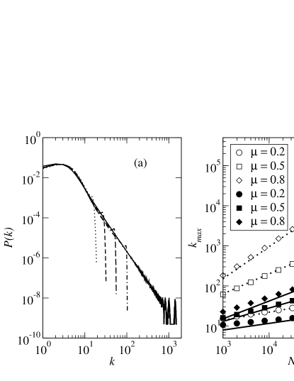
Figure 1: (a) Degree distributions of the static model (solid line) with $N=2^{9}\times 10^{3}$ and the correlated static model with $N=10^{3}$ ($\cdots$), $2^{3}\times 10^{3}$ (- - -), $2^{6}\times 10^{3}$ (– – –), and $2^{9}\times 10^{3}$ (-$\cdot$-$\cdot$-) with $\mu=0.5$ and link density $\delta=K/N=2.0$. (b) Scaling of the maximum degree at $\mu=0.2$, $0.5$, and $0.8$. Open symbols are for the static model and closed symbols are for the correlated static model. Solid lines have slope $1/\lambda=\mu/(1+\mu)$ and dotted lines have slope $1/(\lambda-1)=\mu$.

We present the degree distributions of the correlated static model and the static model with $\mu=0.5$ in Figure 1(a). This confirms the theoretical prediction that both models have the power-law degree distribution with the same degree exponent $\lambda$. However, we find that the maximum cutoff degree $k_{max}$ scales differently with the network size $N$. The maximum degree $k_{max}$ is known to scale as $k_{max}\sim N^{1/(\lambda-1)}$ in the static model Lee04 . This can be derived from the condition that the number of nodes with $k>k_{max}$ should be of the order of unity. This condition demands that $\int_{k_{max}}^{\infty}p(k)dk\sim\int_{k_{max}}^{\infty}k^{-\lambda}dk=\mathcal{O}(1/N)$, which leads to $k_{max}\sim N^{1/(\lambda-1)}$. On the other hand, as one can see in Figure 1(b), $k_{max}$ in the correlated static model is much smaller than that in the static model. The following argument explains the scaling behavior of $k_{max}$. In the correlated static model, one can add a link to a vertex only if there exists another node with the same degree. So, if a node has the maximum degree $k_{max}$, there should be another node having the same degree $k_{max}$. This leads to the constraint $p(k_{\max})=\mathcal{O}(1/N)$ instead of $\int_{k_{max}}^{\infty}p(k)dk=\mathcal{O}(1/N)$. This gives

$$k_{max}\sim N^{1/\lambda}\ .$$ (4)

The numerical data in Figure 1(b) are in good agreement with the scaling behavior in Eq. (4).

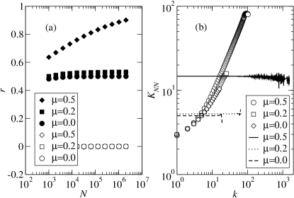
Figure 2: (a) Assortativity coefficient of the static model (open symbols) and the correlated static model (closed symbols). (b) $K_{NN}$ vs. $k$ in the static model (lines) and the correlated static model (symbols) with $N=512000$ vertices.

In order to examine the DD correlation, we measure the assortativity coefficient $r$ Newman02 . This is defined as

$$r=\frac{\langle k_{e,1}k_{e,2}\rangle_{e}-\langle(k_{e,1}+k_{e,2})/2\rangle_{e}^{2}}{\langle(k_{e,1}^{2}+k_{e,2}^{2})/2\rangle_{e}-\langle(k_{e,1}+k_{e,2})/2\rangle_{e}^{2}},$$ (5)

where $\langle(\cdot)\rangle_{e}$ represents the average over all edges, and $k_{e,1}$ and $k_{e,2}$ denote the degrees of two vertices connected with an edge $e$. It is measured and presented in Figure 2(a). While the assortativity coefficients vanish as $N$ increases in the static model, they converge to a finite value as $N$ increases in the correlated static model. Positive correlation is also observed in the mean neighbor degree $K_{NN}(k)$ presented in Figure 2(b). In the correlated static model $K_{NN}(k)\sim k$, while $K_{NN}(k)$ is a constant function in the static model. This shows that the correlated static model has the desired property.

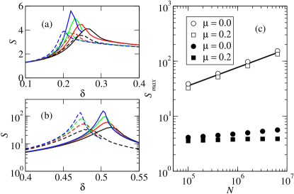
Figure 3: (a) $S$ vs. $\delta$ for the correlated static model (a) and the static model (b) at $\mu=0$ (solid lines) and $0.2$ (dotted lines). Network sizes are $N=10^{5}$, $4\times 10^{5}$, $16\times 10^{5}$, and $64\times 10^{5}$. The larger $N$ is, the higher the peak is. (c) Peak height $S_{max}$ vs. $N$. Closed symbols are for the correlated static model, and open symbols are for the static model. The solid line has slope $1/3$.

III Percolation transition

As a static-model network does Lee04 , so also a correlated model network undergoes a percolation transition as one increases the edge density $\delta\equiv K/N$. To a given value of $\delta$, vertices are decomposed into disjoint sets (called clusters) in such a way that all vertices in a cluster are mutually connected, while those in different clusters are not. The size $s$ of a cluster is defined as the number of vertices in it. When there is no edge ($\delta=0$), each vertex belongs to a cluster of size $s=1$. As edges are added, small clusters merge into large ones. A cluster configuration can be characterized by the cluster size distribution $n_{s}$, which is defined as the ratio of the number of clusters of size $s$ to $N$.

The order parameter for the percolation transition is given by

$$P_{\infty}\equiv\frac{s_{max}}{N},$$ (6)

where $s_{max}$ is the size of the largest cluster. A network is said to be in a percolating phase if $P_{\infty}$ is finite in the $N\rightarrow\infty$ limit. In that case, the largest cluster is called the infinite or giant cluster. If $P_{\infty}$ vanishes in the $N\rightarrow\infty$ limit, a network is said to be in a non-percolating phase. Another useful quantity is the mean cluster size $S$, given by

$$S\equiv\frac{\sum^{\prime}_{s}s^{2}n_{s}}{\sum^{\prime}_{s}sn_{s}},$$ (7)

where the summation is over all clusters except for the largest cluster.

In the static model, the percolation transition is characterized by power-law scalings, $P_{\infty}\sim(\delta-\delta_{c})^{\beta}$ and $S\sim|\delta-\delta_{c}|^{-\gamma}$ for $\lambda>3$, where $\delta_{c}=(1-2\mu)/(2(1-\mu)^{2})$ is the percolation threshold. The critical exponents have the values $\beta=1$ and $\gamma=1$ for $\lambda>4$, and $\beta=1/(\lambda-3)$ and $\gamma=1$ for $3<\lambda<4$ Lee04 . When $\lambda\leq 3$, the networks are always in the percolating phase.

We perform numerical studies of the percolation transition in the correlated static model and compare the results with those of the static model. A striking difference is observed in the behavior of the mean cluster size $S$. In Figure 3, we compare $S$ obtained for the static and correlated static models at $\mu=0$ and $0.2$. In the static-model cases, there are peaks in the plot of $S$ near percolation thresholds, which sharpen as $N$ increases. Theoretically, the peak heights should grow algebraically as $S_{max}\sim N^{\gamma/\bar{\nu}}$ with the finite-size-scaling exponent $\bar{\nu}=3$ for $\lambda>4$ and $\bar{\nu}=(\lambda-1)/(\lambda-3)$ for $3<\lambda<4$ Lee04 . Our data are consistent with the power-law scaling for the static model.

On the other hand, in the correlated-static-model cases, the peaks are not as sharp as in the static model. The peak heights seem to converge to a finite value or at most scale logarithmically with $N$. The weak singular behavior of $S$ suggests that the percolation transition in the correlated static model does not belong to the same universality as that in the uncorrelated static model.

In order to characterize the phase transition, we study finite-size-scaling behaviors of the order parameter $P_{\infty}$ near percolation thresholds. At criticality, we expect that $P_{\infty}$ scales algebraically as

$$P_{\infty}(N)\sim N^{-\alpha}.$$ (8)

The asymptotic value of the scaling exponent $\alpha$ is obtained from the analysis of the effective exponent $\alpha_{e}(N,\delta)\equiv-\ln(P_{\infty}(mN,\delta)/P_{\infty}(N,\delta))/\ln m$ with constant $m=4$. If $P_{\infty}$ follows the power law, then the effective exponent will converge to the scaling exponent in the $N\rightarrow\infty$ limit. Otherwise, it will converge to a trivial value of $0$ or $1$.

Figure 4: Plot of the effective exponent $\alpha_{e}(N,\delta)$ in the correlated static model with $\mu=0.0$ (a) and $\mu=0.2$ (b), and in the static model with $\mu=0.0$ (c) and $\mu=0.2$ (d). Circle, square, and diamond symbols are used for $N=(1,4,16)\times 10^{5}$, respectively.

In Figure 4, we present a plot of $\alpha_{e}(N,\delta)$ for the static model and the correlated static model. We find a significant difference in finite-size-scaling behaviors of $\alpha_{e}$. First, consider the correlated static model shown in Figure 4(a) and (b). At large values of $\delta$, $\alpha_{e}$ vanishes as $N$ increases, which indicates that the system is in the percolating phase with finite $P_{\infty}$. On the other hand, at small values of $\delta$, it converges to a nontrivial value $\alpha<1$ that varies continuously with $\delta$. This suggests that the correlated static model is critical not only at the percolation threshold but also in the entire non-percolating phase. We estimate the percolation threshold as the point at which the power-law scaling sets in. The results are $\delta_{c}=0.19(1)$ at $\mu=0.0$ and $\delta_{c}=0.15(1)$ at $\mu=0.2$. At the transition point, the scaling exponent takes the value

$$\alpha_{c}=0.5(1)$$ (9)

in both cases with $\mu=0.0$ and $0.2$.

The unusual scaling behavior of $P_{\infty}$ in the correlated static model becomes clear when one compares it with that in the static model. Figure 4(c) and (d) show that the static-model networks are critical only at the percolation thresholds, $\delta_{c}\simeq 0.50$ at $\mu=0.0$ and $\delta_{c}\simeq 0.47$ at $\mu=0.2$. The scaling exponent at the critical point is given by $\alpha_{c}\simeq 0.33$. These numerical results are in good agreement with the analytic results Lee04 .

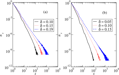
Figure 5: Cluster size distribution, $n_{s}$, in the non-percolating phase of the correlated static model with $\mu=0.0$ (a) and $0.2$ (b).

In order to investigate further the criticality in the non-percolating phase, we study the cluster size distribution, $n_{s}$. Figure 5 shows $n_{s}$ at $\delta\leq\delta_{c}$ in the correlated static model with $\mu=0.0$ and $0.2$. We find that the cluster size distribution follows a power-law distribution $n_{s}\sim s^{-\tau}$ with varying exponent $\tau$. This result also suggests that the correlated static model is critical in the entire non-percolating phase.

We also studied the percolation transition at larger values of $\mu$ (smaller value of $\lambda$). In the static model, networks are always in the percolating phase ($\delta_{c}=0$) if $\mu\geq 1/2$ or $\lambda\leq 3$ Lee04 . However, our numerical data show that the percolation threshold in the correlated static model already vanishes at $\mu=1/4$ ($\lambda=5$). This implies that the correlated static model network is more robust than the static model network.

IV Summary

We have introduced a correlated static model and investigated the nature of the percolation transition. Interestingly, the correlated static model is critical in the entire non-percolating phase below the percolation threshold. That is, the percolation order parameter scales algebraically as $P_{\infty}\sim N^{-\alpha}$ and the cluster size distribution follows the power law as $n_{s}\sim s^{-\tau}$ with varying exponents $\alpha$ and $\tau$. Such a type of percolation transition is also observed in the growing-network models and the assortative exponential random-graph model. These results support the claim that the assortative DD correlation may give rise to a structural correlation which is responsible for novel type of percolation transition.

- (1) D. J. Watts and S. H. Strogatz, Nature (London) 393, 440 (1998).
- (2) R. Albert and A.-L. Barabási, Rev. Mod. Phys. 74, 47 (2002).
- (3) S. N. Dorogovtsev and J. F. F. Mendes, Adv. Phys. 51, 1079 (2002).
- (4) M. E. J. Newman, SIAM Rev. 45, 167 (2003).
- (5) S. H. Lee and H. Jeong, J. Korean Phys. Soc. 48, 186 (2006).
- (6) J. D. Noh and S.-W. Kim, J. Korean Phys. Soc. 48, 202 (2006).
- (7) J. D. Noh, J. Korean Phys. Soc. 50, 327 (2007).
- (8) M. E. J. Newman, Phys. Rev. Lett. 89, 208701 (2002).
- (9) A. Vázquez and Y. Moreno, Phys. Rev. E 67, 015101(R) (2003).
- (10) M. Á. Serrano and M. Boguñá, Phys. Rev. Lett. 97, 088701 (2006); Phys. Rev. E 74, 056114 (2006); Phys. Rev. E 74, 056115 (2006).
- (11) H. Rozenfeld and D. ben-Avraham, Phys. Rev. E 75, 061102 (2007).
- (12) R. Pastor-Satorras, A. Vázquez and A. Vespignani, Phys. Rev. Lett. 87, 258701 (2001).
- (13) A. Vázquez, R. Pastor-Satorras and A. Vespignani, Phys. Rev. E 65, 066130 (2002).
- (14) J. D. Noh, Phys. Rev. E 76 026116 (2007).
- (15) D. S. Callaway, J. E. Hopcroft, J. M. Kleinberg, M. E. J. Newman and S. H. Strogatz, Phys. Rev. E 64, 041902 (2001).
- (16) S. N. Dorogovtsev, J. F. F. Mendes and A. N. Samukhin, Phys. Rev. E 64, 066110 (2001).
- (17) J. Kim, P. L. Krapivsky, B. Kahng and S. Redner, Phys. Rev. E 66, 055101(R) (2002).
- (18) P. L. Krapivsky and B. Derrida, Physica A 340, 714 (2004).
- (19) J. D. Noh, arXiv:0707.0560 (2007).
- (20) K.-I. Goh, B. Kahng and D. Kim, Phys. Rev. Lett. 87, 278701 (2001).
- (21) J.-S. Lee, K.-I. Goh, B. Kahng and D. Kim, Eur. Phys. J. B 49, 231 (2006).
- (22) D.-S. Lee, K.-I. Goh, B. Kahng and D. Kim, Nucl. Phys. B 696, 351 (2004).