Abstract

We consider non-standard matter effect in flavor conversion of neutrinos crossing the core of the Earth. We show that oscillation of core crossing neutrinos with $E\lower 3.01385pt\hbox{$\;\stackrel{{\scriptstyle\textstyle>}}{{\sim}}\;$}0.5$ GeV can be well described by a first order perturbation theory. We show that due to non-standard matter effect varying chemical composition in the Earth can modify the neutrino flavor conversion by $100\%$. Effects of CP violating phases in non-standard Neutral Current interactions are emphasized in particular.

PACS: 14.60.Pq, 13.15.+g

1 Introduction

It is well known that non-standard interaction(NSI) can induce non-standard matter effect for neutrino oscillation in medium. Neutrino flavor conversion induced by non-standard matter effect was proposed as a candidate solution to the solar neutrino anomaly [1]. The present experiments told us that LMA MSW solution [1, 2] with the standard interaction is the solution to the solar neutrino problem [3, 4, 5, 6]. Non-standard matter effect is small in oscillation of solar neutrinos. However non-standard matter effect can be much larger for neutrinos with high energy ($E\lower 3.01385pt\hbox{$\;\stackrel{{\scriptstyle\textstyle>}}{{\sim}}\;$}10$ GeV), e.g. for long baseline neutrinos, atmospheric neutrinos, cosmic neutrinos from the galactic or extra-galactic sources. This is because flavor conversion induced by flavor mixing in vacuum decreases as energy increases while the matter effect does not decrease with energy. Previous works on effect of NSI in neutrino oscillation include  [7, 8].

Non-standard matter effect can be induced by non-standard Neutral Current interaction of neutrinos with electron, proton and neutron. In this respect non-standard matter effect in neutrino oscillation is not only a way to probe physics beyond the Standard Model but also a way to probe chemical composition in matter. Incorporating non-standard matter effect in neutrino oscillation introduces more CP violating phases in the Hamiltonian. These CP violating phases interfere with the CP violating phase in vacuum and can give interesting phenomena. In matter with varying chemical composition these CP violating phases can contribute with different combinations in observables.

It is the purpose of the present article to study the effect of varying chemical composition in the Earth. Effects of CP violating phases in the non-standard interaction will be analyzed in particular. In section 2 we show that oscillation of core crossing neutrinos in the Earth can be well described by a first order perturbation theory which was developed in a previous paper by the author. Scenarios with different CP violating phases and varying composition in the Earth are shown. In section 3 we show the effect of non-standard interactions and CP violating phases in the non-standard interactions. We summarize and comment in section 4. We do analysis using the density profile of the Preliminary Earth Model(PREM)  [9].

2 Non-standard matter effect in the Earth

We consider oscillation of three flavors of neutrinos: $\psi=(\nu_{e},\nu_{\mu},\nu_{\tau})$. The evolution equation is

$$i\frac{d}{dx}\psi(x)=H(x)\psi(x),$$ (1)

where

$$H(x)=H_{0}+V(x),$$ (2)

$$H_{0}=\frac{1}{2E}U~{}\textrm{diag}\{0,\Delta m^{2}_{21},\Delta m^{2}_{31}\}~{}U^{\dagger}.$$ (3)

$V(x)$, a $3\times 3$ matrix, is the potential term accounting for the matter effect. $U$ is the $3\times 3$ neutrino mixing matrix in vacuum. $U$ is parameterized using standard parameters $\theta_{12}$, $\theta_{13}$, $\theta_{23}$ and $\delta_{13}$, the CP violating phase.

In the presence of non-standard NC interaction the potential term can be written as follows

$$V(x)=\textrm{diag}\{V_{e},0,0\}+\begin{pmatrix}0&V_{e\mu}&V_{e\tau}\cr V_{\mu e}&V_{\mu\mu}&V_{\mu\tau}\cr V_{\tau e}&V_{\tau\mu}&V_{\tau\tau}\end{pmatrix},$$ (4)

where $V_{e}=\sqrt{2}G_{F}N_{e}$ is the potential with standard charged current interaction. $G_{F}$ is Fermi constant and $N_{e}$ is electron number density. $V_{kl}$ is from non-standard NC interaction. $V_{lk}^{*}=V_{kl}$ because the Hamiltonian is hermitian. $x$ dependence in $V_{kl}$ has been suppressed in Eq. (4). $V_{ee}$ has been made zero in our convention. This is achieved by shifting the phases of neutrinos: $\nu_{l}\to e^{-i\int dx~{}V_{ee}}~{}\nu_{l}$.

In this convention $V_{kl}$ is

$$V_{kl} =\sqrt{2}G_{F}~{}\sum_{s=e,p,n}(f^{s}_{kl}-f^{s}_{ee})N_{s}$$ (5)

$$=V_{e}~{}[\sum_{s=e,p,n}(f^{s}_{kl}-f^{s}_{ee})+(f^{n}_{kl}-f^{n}_{ee})R_{n}],,$$

where

$$R_{n}=(N_{n}-N_{e})/N_{e}.$$ (6)

$f^{e}_{kl}$, $f^{p}_{kl}$ and $f^{n}_{kl}$ are the dimensionless strengths of non-standard four Fermion interactions $\sqrt{2}~{}f^{s}_{kl}~{}G_{F}~{}{\bar{s}}\gamma_{\mu}s~{}{\bar{\nu}_{k}}\gamma^{\mu}\nu_{l}$. $N_{p}$ and $N_{n}$ are number densities of proton and neutron in matter. In obtaining the second line of Eq. (5) $N_{e}=N_{p}$ in neutral matter has been used.

We can re-write $V(x)$ as

$$V(x)=V_{e}(x)\begin{pmatrix}1&\epsilon_{e\mu}&\epsilon_{e\tau}\cr\epsilon_{\mu e}&\epsilon_{\mu\mu}&\epsilon_{\mu\tau}\cr\epsilon_{\tau e}&\epsilon_{\tau\mu}&\epsilon_{\tau\tau}\end{pmatrix}.$$ (7)

where $\epsilon_{kl}=V_{kl}/V_{e}$. We can write

$$\epsilon_{kl}=\epsilon^{0}_{kl}(1+R_{n}~{}r_{kl}~{}e^{-i\phi_{kl}}),$$ (8)

where

$$\epsilon^{0}_{kl}=\sum_{s=e,p,n}(f^{s}_{kl}-f^{s}_{ee}),~{}r_{kl}~{}e^{-i\phi_{kl}}=(f^{n}_{kl}-f^{n}_{ee})/\epsilon^{0}_{kl}.$$ (9)

$\epsilon^{0}_{kl}$ is constant in matter. $\epsilon_{kl}$ depends on the chemical composition in matter and may have $x$ dependence in neutrino trajectory. $r_{kl}$ and $\phi_{kl}$ are real numbers. $\epsilon^{0}_{ee}=0$ and $r_{ee}=0$ in our convention. $\epsilon^{0}_{kl}=\epsilon^{0*}_{lk}$ and $\phi_{kl}=-\phi_{lk}$ because of the hermiticity of $V$.

Constraints on $\epsilon_{kl}$ come from direct test on NSI [10, 11] and the neutrino oscillation experiments. Test on NSI can not be directly translated to constraint on $\epsilon_{kl}$. These constraints have been discussed in our previous work [12]. It was shown that present constraints are $|\epsilon_{\mu\mu}|,|\epsilon_{\tau\tau}|\lower 3.01385pt\hbox{$\;\stackrel{{\scriptstyle\textstyle<}}{{\sim}}\;$}10^{-2}$ and $|\epsilon_{\mu e}|,|\epsilon_{\mu\tau}|\lower 3.01385pt\hbox{$\;\stackrel{{\scriptstyle\textstyle<}}{{\sim}}\;$}10^{-2}$, $|\epsilon_{e\tau}|\lower 3.01385pt\hbox{$\;\stackrel{{\scriptstyle\textstyle<}}{{\sim}}\;$}10^{-1}$ [12, 13, 14].

It is clear that $\epsilon^{0}_{kl}$ introduces three CP violating phases in addition to the phase $\delta_{13}$ in matrix $U$. They are phases of $\epsilon^{0}_{e\mu,e\tau,\mu\tau}$. Furthermore $\phi_{e\mu,e\tau,\mu\tau}$ become independent phases in case that chemical composition varies in matter. So in matter with varying chemical composition, i.e. $R_{n}$ not a constant, we have seven physical CP violating phases in total. They can give interesting phenomena in neutrino oscillation. In Earth matter $R_{n}$ is estimated[15]

$$R_{n}=\left\{\begin{matrix}0.024,&\textrm{~{}~{}~{}mantle}\cr 0.146,&\textrm{core}\end{matrix}\right.$$ (10)

We will use numbers in (10) in our analysis in the present article. We will concentrate on neutrinos with core crossing trajectories.

It was shown in a previous work that oscillation of neutrinos in the Earth can be well described by a first order perturbation theory [12, 16]. The theory was analyzed with the assumption that $\epsilon_{kl}$ is a constant in neutrino trajectory. We show in this section that this theory works perfectly well taking into account the fact that chemical composition in the core and in the mantle are different.

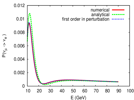
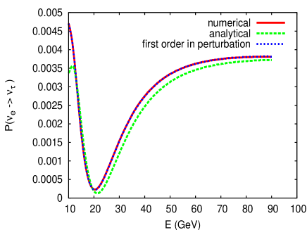
Figure 1: Left $P(\nu_{\mu}\to\nu_{e})$ versus energy; right $P(\nu_{e}\to\nu_{\tau})$ versus energy. $L=12000$ km, $\Delta m^{2}_{21}=8.\times 10^{-5}$ eV², $\Delta m^{2}_{32}=3.\times 10^{-3}$ eV². $\sin^{2}2\theta_{23}=1$, $\tan^{2}\theta_{12}=0.41$, $\sin^{2}2\theta_{13}=0.01$, $\delta_{13}=\pi/6$. $\epsilon^{0}_{e\mu}=0.01~{}e^{-i\pi/20}$, $\epsilon^{0}_{e\tau}=0.04~{}e^{-i\pi/3}$, $\epsilon^{0}_{\mu\tau}=0.01~{}e^{-i\pi/20}$. $r=5$, $\phi_{e\mu}=\phi_{\mu\tau}=\pi/2$, $\phi_{e\tau}=0$. PREM density profile is used for computation in this figure and all remaining figures in this article.

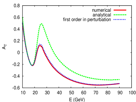
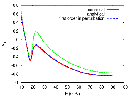
Figure 2: Time reversal asymmetry, $A_{T}$, versus energy. Left $r=5$; right $r=2$. Other parameters are the same as in Fig. 1.

We quickly review the perturbation theory. We denote $L$ as the length of neutrino trajectory in the Earth. For core crossing neutrinos($L\lower 3.01385pt\hbox{$\;\stackrel{{\scriptstyle\textstyle>}}{{\sim}}\;$}10690$ km) we write the evolution matrix $M$ as

$$M=M_{3}M_{2}M_{1},$$ (11)

where $M_{2}$ is the evolution matrix in the core and $M_{1,3}$ are evolution matrices in the mantle. $0<x<L_{1}$ and $L_{2}<x<L$ are the parts of trajectory in the mantle; $L_{1}<x<L_{2}$ is the part of trajectory in the core. We average potential in the mantle and in the core separately

$${\bar{V}}_{i}=\frac{1}{L_{i}-L_{i-1}}\int^{L_{i}}_{L_{i-1}}~{}dx~{}V(x),~{}~{}~{}i=1,2,3,$$ (12)

where $L_{3}=L$. Using ${\bar{V}}_{i}$ we define the average Hamiltonian

$${\bar{H}}_{i}=H_{0}+{\bar{V}}_{i},~{}~{}i=1,2,3$$ (13)

and get eigenvector and mixing matrix

$${\bar{H}}U_{mi}=U_{mi}~{}\frac{\Delta_{i}}{2E},~{}~{}i=1,2,3.$$ (14)

$\Delta_{i}$ is a vector. The evolution matrix $M_{i}$ is expressed as

$$M_{i} =U_{mi}~{}e^{-i\frac{\Delta_{i}}{2E}(L_{i}-L_{i-1})}(1-iC^{i})~{}U^{\dagger}_{mi},~{}~{}i=1,2,3$$ (15)

$C^{i}$ is a $3\times 3$ matrix accounting for the non-adiabatic transition:

$$C^{i}=\int^{L_{i}}_{L_{i-1}}dx~{}e^{i\frac{\Delta_{i}}{2E}x}~{}U^{\dagger}_{mi}~{}\delta V_{i}(x)~{}U_{mi}~{}e^{-i\frac{\Delta_{i}}{2E}x},$$ (16)

where

$$\delta V_{i}(x)=V(x)-{\bar{V}}_{i}.$$ (17)

It is clear that $(C^{i})^{\dagger}=C^{i}$ holds.

In [12] we have discussed in detail that this theory is indeed doing expansion using small quantities. $C^{i}_{jk}(j\neq k)$ is suppressed by small quantities for neutrinos with $E\lower 3.01385pt\hbox{$\;\stackrel{{\scriptstyle\textstyle>}}{{\sim}}\;$}0.5$ GeV. Second order effect is of order ${\cal O}(C^{2})$ and is further suppressed.

In Fig. 1 we compare the result of numerical computation with that computed in the first order perturbation theory, i.e. using Eqs. (11) and (15). For simplicity we have set

$$\epsilon_{\mu\mu}=\epsilon_{\tau\tau}=0,~{}~{}r_{e\mu}=r_{e\tau}=r_{\mu\tau}=r.$$ (18)

We see that result computed using the perturbation theory is in remarkable agreement with the numerical result.

We also show the zeroth order result, i.e. result computed by setting $C_{i}$ zero in Eq. (11). The zeroth order result is an analytical result computed using average potentials in the core and in the mantle separately. We see that the analytical result is not a bad approximation to the oscillation pattern. It qualitatively describes the neutrino oscillation pattern and can help a lot when making qualitative discussions.

In Fig 2 we show plot of time reversal asymmetry versus energy. $A_{T}$ is defined as

$$A_{T} =\frac{P(\nu_{e}\to\nu_{\mu})-P(\nu_{\mu}\to\nu_{e})}{P(\nu_{e}\to\nu_{\mu})+P(\nu_{\mu}\to\nu_{e})}.$$ (19)

Again we see that the first order perturbation theory gives a perfect description of the oscillation pattern. The analytical result gives a qualitatively good approximation to neutrino oscillation. It can help in making qualitative discussions.

3 Flavor conversion of core crossing neutrinos

In this section we illustrate the effect of CP violating phases of NSI in neutrino oscillation.

As shown in the last section, oscillation of core-crossing neutrino can be qualitatively described by approximation which uses average densities in the mantle and in the core separately. This is an analytical description. We use this description to simplify the discussion and see the effect of $\phi_{kl}$ in neutrino oscillation.

It is easier to discuss in the large energy region where we can re-write the Hamiltonian as

$$H=V_{0}+H_{1},$$ (20)

where

$$V_{0}=\textrm{diag}\{V_{e},0,0\},~{}~{}H_{1}=V-V_{0}+H_{0}.$$ (21)

$V_{0}$ is taken as the leading term in the Hamiltonian. $H_{1}$ is taken as perturbation. $V-V_{0}$ is for the non-standard matter effect and $H_{0}$ is the Hamiltonian in vacuum. $H_{0}$ decreases as energy increases.

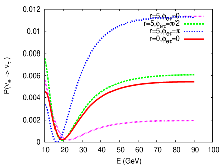
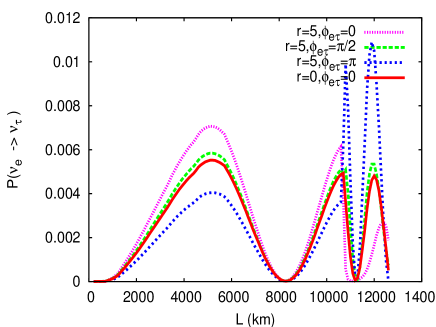
Figure 3: $P(\nu_{e}\to\nu_{\tau})$ versus energy, $L=12000$ km; $P(\nu_{e}\to\nu_{\tau})$ versus distance L, $E=50$ GeV. $\phi_{e\mu}=\phi_{\mu\tau}=\pi/2$. Other parameters are the same as in Fig. 1.

Using the average potentials in the core and in the mantle we can get the evolution matrix using perturbation in $H_{1}$. As an example, $\nu_{e}\to\nu_{\tau}$ amplitude is

$$A(\nu_{e}\to\nu_{\tau}) \approx\frac{(H^{m}_{1})_{\tau e}}{V^{m}_{e}}(e^{-i\varphi_{1}}-1)+\frac{(H^{c}_{1})_{\tau e}}{V^{c}_{e}}(e^{-i\varphi_{c}}-1)e^{-i\varphi_{1}}$$ (22)

$$+\frac{(H^{m}_{1})_{\tau e}}{V^{m}_{e}}(e^{-i\varphi_{1}}-1)e^{-i(\varphi_{c}+\varphi_{1})},$$

where $\varphi_{c}=V^{c}_{e}(L_{2}-L_{1})$ and $\varphi_{1}=V^{m}_{e}L_{1}$. $H^{m}_{1}$ and $H^{c}_{1}$ are averages of $H_{1}$ in the mantle and in the core. $V^{m}_{e}$ and $V^{c}_{e}$ are averages of $V_{e}$ in the mantle and in the core. The property of approximately symmetric density profile in the Earth has been used in Eq. (22). It can be written as

$$A(\nu_{e}\to\nu_{\tau})\approx\frac{(H^{m}_{1})_{\tau e}}{V^{m}_{e}}(e^{-i\varphi}-1)+(\frac{H^{c}_{1}}{V^{c}_{e}}-\frac{H^{m}_{1}}{V^{m}_{e}})_{\tau e}(e^{-i\varphi_{c}}-1)e^{-i\varphi_{1}},$$ (23)

where $\varphi=\varphi_{c}+2\varphi_{1}$.

Neglecting terms of order ${\cal O}(\frac{\Delta m^{2}_{21}}{2EV_{e}},\frac{\Delta m^{2}_{31}}{2EV_{e}}\sin\theta_{13})$, we get

$$A(\nu_{e}\to\nu_{\tau}) \approx\epsilon^{0}_{\tau e}~{}(1+0.024~{}r_{\tau e}~{}e^{-i\phi_{\tau e}})(e^{-i\varphi}-1)$$ (24)

$$+0.122~{}\epsilon^{0}_{\tau e}~{}r_{\tau e}~{}e^{-i\phi_{\tau e}}(e^{-i\varphi_{c}}-1)e^{-i\varphi_{1}}.$$

Eq. (10) has been used in obtaining Eq. (24). $A(\nu_{e}\to\nu_{\tau})$ is determined by $\epsilon^{0}_{\tau e}$ modulated by contribution of $r_{\tau e}$ and $\phi_{\tau e}$. For neutrinos which do not cross the core of the Earth the second term in the r.h.s. of Eq. (24) is absent.

One can see clearly in Eq. (24) that if $r_{\tau e}=0$ the transition amplitude, $A(\nu_{e}\to\nu_{\tau})$, is determined by $\epsilon^{0}_{\tau e}$ and modulated by factor $e^{-i\varphi}-1$. Hence $P_{e\tau}$ is proportional to function $\sin^{2}(\varphi/2)$. In the right panel of Fig. 3 we see plot for this case. For $r_{\tau e}=0$ and $\phi_{\tau e}=0$, $P_{e\tau}$ has three peaks with roughly equal heights, as expected. For $r_{\tau e}=5$, $P_{e\tau}$ is considerably changed. When $\varphi_{\tau e}=0$ and $\varphi_{\tau e}=\pi$, $P_{e\tau}$ is considerably modified around the third peak (for core-crossing neutrinos). The height in this peak is quite different from that in the first peak (for neutrinos crossing the mantle only). This is quite different from the case with $r_{\tau e}=0$. In the left panel of Fig. 3 we show the plots of transition probability versus energy. Again we see the effect of $r_{\tau e}$ and $\varphi_{\tau e}$. $P_{e\tau}$ is also slightly modified in the first peak when $r_{\tau e}\neq 0$. This is because of the correction by $r_{\tau e}$ to the Hamiltonian in the mantle, as shown in the first term in the r.h.s of Eq. (24). Comparing with the transition probability in neutrinos crossing the mantle, the core-crossing neutrino events encode the information of $r_{\tau e}$ and $\varphi_{\tau e}$. And effect of $\epsilon^{0}_{kl}$ and $r_{kl}$ are distinctly different in oscillation probability.

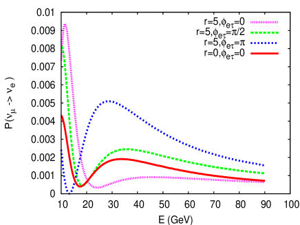
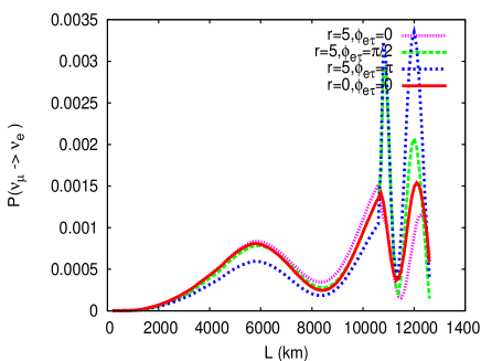
Figure 4: $P(\nu_{\mu}\to\nu_{e})$ versus energy, $L=12000$ km; $P(\nu_{\mu}\to\nu_{e})$ versus distance L, $E=50$ GeV. $\phi_{e\mu}=\phi_{\mu\tau}=\pi/2$. Other parameters are the same as in Fig. 1.

In Fig. 3 we see that when $L=12000$km $P_{e\tau}$ is reduced when $\varphi_{\tau e}=0$ and is enhanced when $\varphi_{\tau e}=\pi$. This phenomenon can be understood by considering an interesting case which happens when

$$\varphi_{c}+\varphi_{1}\approx 2n\pi,$$ (25)

where $n$ is an integral. Hence $\varphi\approx\varphi_{1}+2n\pi$. This is the region of parametric resonance for oscillation with standard matter effect [18, 19]. In the presence with non-standard matter effect we see that the amplitude is not always enhanced. Using Eqs. (24) and (25) we get

$$A(\nu_{e}\to\nu_{\tau}) \approx\epsilon^{0}_{\tau e}~{}(1-0.098~{}r_{\tau e}~{}e^{-i\phi_{\tau e}})(e^{-i\varphi}-1).$$ (26)

The amplitude is reduced for $\phi_{\tau e}=0$ and is enhanced for $\phi_{\tau e}=\pi$. When $r=5$ the transition probability is reduced or enhanced by $100\%$. When $\phi_{e\tau}=\pi/2$ $P_{e\tau}$ is not much enhanced. This is understood by noting that according to Eq. (26) $P_{e\tau}$ is enhanced by factor $1+(0.098r)^{2}\approx 1+0.01r^{2}$. It is a $25\%$ increase when $r=5$. In Fig. 4 we plot $P(\nu_{\mu}\to\nu_{e})$ versus energy and the distance L. We can also see the effect of $r_{kl}$ and $\phi_{kl}$ in this plot. In the right panel of Fig. 4 significant modifications are seen in the second and third peaks.

4 Conclusions

In summary we have analyzed non-standard matter effect in flavor conversion of neutrinos crossing the core of the Earth. We have shown that a first order perturbation theory gives a perfect description of neutrino oscillation for core-crossing trajectories. The analytical description, which uses only zeroth order result, gives a good approximation.

One interesting thing is that there are six physical CP violating phases associated with the non-standard matter effect when chemical composition changes in matter. This is what happens to core crossing neutrinos. It is different from the case when chemical composition does not change. In the latter case there are only three physical CP violating phases. We analyze effect of additional CP violating phases in neutrino oscillation.

We have shown that due to non-standard interaction different chemical composition in the core and the mantle ( different $N_{n}/N_{e}$ ) can modify neutrino flavor conversion by $100\%$. We analyze in particular the region of parametric resonance. It is shown that in this region the non-standard matter effect does not always give enhancement to the amplitude. Depending on the CP violating phases the non-standard matter effect reduce or enhance the neutrino flavor conversion. The signature of non-standard interactions lies in the dependence of the neutrino flavor conversion rate on $E$, the energy of neutrinos, and $L$, the length of neutrino trajectory in the Earth. To figure out these interactions we need neutrino sources with different energies and baselines.

The analysis presented in the present article shows that core crossing neutrino events provide an interesting way to test interactions of neutrinos beyond the Standard Model. They also provide an independent way to test chemical composition in the Earth.

Acknowledgment: The research is supported in part by National Science Foundation of China(NSFC), grant 10745003.

References

- [1] L. Wolfenstein, Phys. Rev. D 17, 2369 (1978); L. Wolfenstein, in ”Neutrino-78”, Purdue Univ. C3 - C6, (1978).
- [2] S. P. Mikheyev and A. Yu. Smirnov, Yad. Fiz. 42, 1441 (1985) [ Sov. J. Nucl. Phys. 42, 913 (1985)]; Nuovo Cim. C9, 17 (1986); S. P. Mikheyev and A. Yu. Smirnov, ZHETF, 91, (1986), [Sov. Phys. JETP, 64, 4 (1986)] (reprinted in ”Solar neutrinos: the first thirty years”, Eds. J.N. Bahcall et. al.).
- [3] Q. R. Ahmad et al., SNO collaboration Phys. Rev. Lett 87, 071301(2001); ibidem 89, 011301(2002); ibidem 89, 011302(2002).
- [4] S. N. Ahmed et al., SNO collaboration, Phys. Rev. Lett. 92, 181301(2004).
- [5] Super-Kamiokande collaboration, S. Fukuda et al., Phys. Rev. Lett. 86, 5651(2001); Phys. Rev. Lett. 86, 5656(2001); Phys. Lett. B 539, 179(2002).
- [6] K. Eguchi et al., KamLAND Coll., Phys. Rev. Lett. 90, 021802(2003).
- [7] M. C. Gonzalez-Garcia, Y. Grossman, A. Gusso, Y. Nir, Phys. Rev. D64, 096006(2001); A. M. Gago, M.M. Guzzo, H. Nunokawa, W. J. C. Teves, R. Z. Funchal, Phys. Rev. D64, 073003(2001) ; P. Huber, T. Schwetz, J. W. F. Valle, Phys. Rev. Lett. 88, 101804(2002); Phys.Rev. D66, 013006(2002); T. Ota, J. Sato, N. Yamashita, Phys. Rev. D65, 093015(2002); T. Ota, J. Sato, Phys. Lett. B545, 367(2002).
- [8] N. Kitazawa, H. Sugiyama, O. Yasuda, arXiv:hep-ph/0606013; A. Friedland, C. Lunardini, Phys. Rev. D74,033012(2006); M. Blennow, T. Ohlsson, J. Skrotzki, arXiv:hep-ph/0702059; M. Honda, N. Okamura, T. Takeuchi, arXiv:hep-ph/0603268; N. C. Ribeiro, H. Minakata, H. Nunokawa, S. Uchinami, R. Zukanovich-Funcha, JHEP0712, 002(2007); M. Blennow, T. Ohlsson, W. Winter, Eur. Phys. J.C49, 1023(2007).
- [9] A.M. Dziewonski and D.L. Anderson, Phys. Earth. Planet. Inter.25, 297(1981).
- [10] G. P. Zeller et al, NuTeV collaboration, Phys. Rev. Lett. 88, 091802 (2002); Erratum 90, 239902 (2003).
- [11] The Review of Particle Physics, W.-M. Yao et al., J. Phys. G33, 1 (2006).
- [12] W. Liao, Phys. Rev. D77, 053002(2008)[arXiv:0710.1492].
- [13] A. Friedland, C. Lunardini , M. Maltoni, Phys. Rev.D70, 111301(2004); A. Friedland, C. Lunardini, Phys. Rev. D72, 053009(2005).
- [14] N. Fornengo, M. Maltoni, R. T. Bayo, J.W.F. Valle, Phys. Rev.D65, 013010(2002); S. Bergmann, M. M. Guzzo, P. C. de Holanda, P.I. Krastev, H. Nunokawa, Phys. Rev. D62, 073001(2000).
- [15] E. Lisi, D. Montanino, Phys. Rev. D56, 1792(1997).
- [16] See also [15] and [17] for ealier works using trajectory dependent average potential.
- [17] E. K. Akhmedov, M. Maltoni, A. Yu. Smirnov, JHEP0705,077(2007).
- [18] E. Kh. Akhmedov, Sov. J. Nucl. Phys. 47, 301(1988).
- [19] Q. Y. Liu and A. Yu. Smirnov, Nucl. Phys. B524, 505(1998); Q. Y. Liu, S. P. Mikheyev, and A. Yu. Smirnov, Phys. Lett. B440, 319(1998); S. T. Petcov, Phys. Lett. B 434, 321(1998); E. Kh. Akhmedov, Nucl. Phys. B538, 25(1999); E. Kh. Akhmedov, A. Dighe, P. Lipari, A. Yu. Smirnov, Nucl. Phys. B542, 3(1999).