Quantum radiations from exciton condensate in Electron-Hole Bilayer Systems

Abstract

Superfluid has been realized in Helium-4, Helium-3 and ultra-cold atoms. It has been widely used in making high-precision devices and also in cooling various systems. There have been extensive experimental search for possible exciton superfluid (ESF) in semiconductor electron-hole bilayer (EHBL) systems below liquid Helium temperature. Exciton superfluid are meta-stable and will eventually decay through emitting photons. Here we find that the light emitted from the excitonic superfluid has unique and unusual features not shared by any other atomic or condensed matter systems. We show that the emitted photons along the direction perpendicular to the layer are in a coherent state with a single energy, those along all tilted directions are in a two modes squeezed state. We determine the two mode squeezing spectra, the angle resolved photon spectrum, the line shapes of both the momentum distribution curve (MDC) and the energy distribution curve (EDC). By studing the two photon correlation functions, we find there are photon bunching, the photo-count statistics is super-Poissonian. We also stress the important difference between the quasi-particle excitations in an equilibrium superfluid and those in a stationary state superfluid. This difference leads to the explanation of recent experimental observation of excitation spectrum of exciton-polariton inside a planar cavity. We discuss how several important parameters such as the chemical potential, the exciton decay rate, the quasiparticle energy spectrum and the dipole-dipole interaction strength between the excitons in our theory can be extracted from the experimental data and comment on available experimental data on both EDC and MDC. We suggest that all the predictions achieved in this paper can be measured by possible future angle resolved power spectrum, phase sensitive homodyne measurements, and HanburyBrown-Twiss type of experiments. We demonstrate explicitly that the photoluminescence from the exciton in EHBL systems is a very natural, feasible and unambiguous internal probe of the nature of quantum phases of excitons in EHBL such as the ground state and the quasi-particle excitations above the ground state. These remarkable features of the photoluminescence can be used for high precision measurements, quantum communication, quantum information processing and also for the development of a new generation of powerful opto-electronic devices.

I Introduction

An Exciton is a bound state of an electron and a hole. Exciton condensate was first proposed more than 3 decades ago as a possible ordered state in solids blatt . Keldysh and Kozlov kel argued that in a bulk semiconductor, in the dilute limit $n_{ex}a^{3}_{ex}\ll 1$ where $n_{ex}$ is the exciton density and $a_{ex}$ is the exciton radius, the excitons behave as weakly interacting bosons, the exciton effective mass $M$ is even smaller than an electron mass, for experimentally accessible exciton densities, the 3 dimensional Bose-Einstein condensation (BEC) critical temperature can be estimated to be $\sim K$. So in principle, the excitons can undergo BEC and become an excitonic superfluid state below a few $K$. In the dense limit $n_{ex}a^{d}_{ex}\gg 1$, the fermionic nature of the electrons and holes in the exciton will show up, the strong pairing BEC superfluid will crossover to weak pairing BCS superfluid old . However, in reality, it is very difficult to realize the BEC of excitons experimentally in a bulk system, because the short lifetime $\tau_{ex}$ and the long lattice relaxation time $\tau_{L}$ which is needed for the hot exciton gas to reach the cold temperature of the underlying lattice by emitting longitudinal acoustic phonons. Although exciton gas, bi-excitons and electron-hole plasma (EHP) phase have been observed in different bulk semi-conductors, no exciton superfluid phase has been observed in any bulk semi-conductors.

Recently, degenerate exciton systems have been produced by different experimental groups with two different methods in quasi-two-dimensional semiconductor $GaAs/AlGaAs$ coupled quantum wells structure butov ; snoke ; field1 ; field2 ; bell . When the distance between the two quantum wells is sufficiently small, an electron in one well and a hole in the other well could pair to form an exciton which behaves as a boson in dilute exciton density limit ( Fig.1a). This kind of inter-layer excitons are called in-direct excitons. In Butov and Snoke’s labs ( also Bell lab ) butov ; snoke ; bell , the excitons are created by optical pumping and then a electric field is applied along the $\hat{z}$ direction to separate electrons from holes by a distance $d\sim 30nm$. There are also the current efforts from Bell lab bell which focused on the effects of electrostatic traps to confine the excitons in a given regime. In the undoped electron-hole bilayer (EHBL) sample prepared in Mike Lilly’ lab field1 ; field2 ; excitonprl ; imbgate ; layerinter ; mag and the Cambridge group camb1 ; camb2 which is a heterostructures insulated-gate field effect transistors, separate gates can be connected to electron layer and hole layer, so the densities of electron and holes can be tuned independently by varying the gate voltages. Low densities and high mobilities regimes for both electrons and holes can be reached. Transport properties such as Coulomb drag can be performed in this experimental set-up.

The quantum degeneracy temperature of a two dimensional excitonic superfluid (ESF) can be estimated to be $T^{ex}_{d}\sim 3K$ for exciton density $n\sim 10^{10}cm^{-2}$ and effective exciton mass $m=0.22m_{0}$ where $m_{0}$ is the bare mass of an electron, so it can be reached easily by $He$ refrigerator. It was established that the indirect excitons in EHBL has at least the following advantages over the excitons in the bulk: (1) Due to the space separation of electrons and holes, the lifetime $\tau_{ex}$ of the excitons is made to be $10^{3}\sim 10^{5}$ longer than that of those in bulk semi-conductors, now it can be made as long as microseconds. Due to the relaxation of the momentum conservation along the $\hat{z}$ direction, the thermal lattice relaxation time $\tau_{L}$ of the indirect excitons can be made as $10^{-3}$ that of bulk excitons, now it can be made as short as nanoseconds. So $\tau_{ex}\gg\tau_{L}$ is well satisfied even for the direct semiconductor such as $GaAs$. (2) Because all the electric dipoles are aligned normal to the 2d plane, the repulsive dipole-dipole interaction is crucial to stabilize the excitonic superfluid against the competing phases such as bi-exciton formation and electron-hole plasma (EHP) phase. So EHBL is a very promising system to observe BEC of in-direct excitons. There are two important dimensionless parameters in the EHBL. One is the dimensionless distance $\gamma=d/a_{B}$ ( $a_{B}$ is the Bohr radius ) between the two layers. Another is $r_{s}$ where $r_{s}a_{B}$ is the typical interparticle distance in a single layer. Recently, one of the authors proposed that the EHBL maybe a more favorable system to observe a metastable excitonic supersolid (ESS) than the Helium 4 system ye . The global phase diagram at $T=0$ labeled by the two parameters is shown in Fig.3.

Figure 1: (a) In the experiments in butov ; snoke ; bell , A laser with excitation power $P_{ex}$ is used to excite electrons from the valence band ( V ) to the conduction band (C) in the semiconductor GaAs/AlGaAs electron-hole bilayer systems. Then a gate voltage $V_{g}$ is applied along the $z$ direction to separate the electrons in the conduction band from the holes in the valence band. One electron in one quantum well and one hole in the other quantum well are bound to form an indirect exciton. In the experiments in field1 ; field2 , the excitons are generated by gate voltages. (b) The geometry of the photon emission from the indirect excitons

Note that in all the previous experiments butov ; snoke ; bell , a laser beam was consistently shined on a given ’bright’ ring ( or a ’bright’ spot ), however, the excitons will move to different locations which is at the center of the ring ( or a ring ) before they annihilate and emit lights ( Fig.2 ). So in the stationary process of emitting lights, the number of the exciton condensation $N$ is kept to be a constant. The laser beam was used to photo-generated the excitons, so it plays the role of a pump, however, because the exciton condensation happens at different locations than the laser pumping point, so if the BEC of excitons indeed happens near the center of the trap, it is indeed spontaneous instead of being stimulated. Indeed, as temperature butov is decreased from $\sim 20K$ to $\sim 1.7K$, the spatially and spectrally resolved PL peak density centering around the gap in Fig.1a $E_{g}\sim 1.545eV$ increases, the exciton cloud size decreases to $L\sim 30\mu m$, the peak width shrinking to $\sim 1meV$ at the lowest temperature $\sim 1.7K$. All these facts indicate the possible formation of exciton condensate around $1.7K$. In our theoretical analysis in this paper, we assume the exciton cloud already reached the lattice temperature by interacting with lattice acoustic phonons within the thermal lattice relaxation time $\tau_{L}$ during its relaxation process to the bottom of the trap, it also become a superfluid through mutual dipole-dipole repulsive interaction and start to radiate photons at the exciton lifetime $\tau_{ex}\gg\tau_{L}$, then we will calculate all the characteristics of the photons emitted from the exciton superfluid. We will compare our theoretical results with the experimental data in Sec.IX. The transient photoluminescence from the excitons created by a short laser pulse will be discussed in a separate publication.

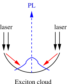
Figure 2: A laser ( black arrow ) with excitation power $P_{ex}$ is used to excite electrons which are relaxed ( red arrow ) to the bottom of the trap, then emit photons ( blue dashed arrow ) spontaneously.

In parallel to search for exciton superfluid in EHBL, extensive activities gold ; hall ; counterflow ; blqhrev ; counterflownature ; fer ; psdw ; imb ; cbtwo have also been lavished on searching for exciton superfluid in electron-electron bilayer system in the same semi-conductor material $AlGaAs/GaAs$ subject to a high magnetic field in quantum Hall regime at total filling factor $\nu_{T}=1$. When the interlayer separation $d$ is sufficiently large, the bilayer system decouples into two separate compressible $\nu=1/2$ layers. However, when $d$ is smaller than a critical distance $d_{c}$, the system may undergo a quantum phase transition into a novel spontaneous interlayer coherent exciton superfluid phase blqhrev . The exciton in this system can be considered as the pairing of an electron in top layer and the hole in the bottom layer after making a particle-hole transformation in the bottom layer. Other phases such as pseudo-spin density wave phase in some intermediate distance regimes was also proposed psdw ; imb ; cbtwo . At low temperature, with extremely small interlayer tunneling amplitude, Spielman et al discovered a very pronounced narrow zero bias peak in this possible exciton superfluid state gold . M. Kellogg et al also observed quantized Hall drag resistance at $h/e^{2}$ hall . In the counterflow experiments, it was found that both linear longitudinal and Hall resistances take activated forms and vanish only in the zero temperature limit counterflow . However, despite the intensive theoretical research blqhrev in the past, there are still many serious discrepancies between theory and the experiments. It remains unclear if the excitonic superfluid was indeed realized in the BLQH system.

It is instructive to compare the measurements to detect possible exciton superfluid in the BLQH and EHBL In the BLQH, there are mainly three kinds of transport experimental measurements (1) Quantum Hall resistance (2) Interlayer tunneling (3) Counterflow. In contrast to these quantum phases in BLQH which are stable ones, all these excitonic phases in EHBL in the Fig.3 are just meta-stable states which will eventually decay by emitting lights. So the most natural experimental measurement for photo generated EHBL is the photoluminescence (PL) which is quite different from all the transport measurements in the BLQH. The geometry of the photoluminescence from EHBL systems is shown in Fig.1b. In fact, the photon emission in EHBL plays a similar role as the interlayer tunneling the BLQH, so the theoretical results achieved in both systems should shed on and transfer lights to each other. Very recently, transport experiments such as Coulomb drag were also performed in EHBL generated by gate voltages field1 ; field2 ; excitonprl ; imbgate ; layerinter ; mag . It is possible to also perform counterflow experiment in the near future. The PL experiment can also be performed in this gate voltage generated EHBL, although the emitted lights are weaker than those from the photo generated EHBL private .

Figure 3: Zero temperature phase diagram of electron and hole bilayer at the balanced case $n_{e}=n_{h}$ ( but $m_{e}\neq m_{h}$ ). The very important effects of spins, traps and disorders are not taken into account. The $d$ is interlayer distance. $r_{s}a_{B}$ where $a_{B}$ is the Bohr radius is the average inter-particle distance in a single layer. At high densities ( low $r_{s}$ ), along the dashed line (I), there is a transition from the weak pairing ( or BCS ) ESF to the electron-hole plasma ( EHP ) phase. At low densities ( high $r_{s}$ ), along the dashed line (II), there is a transition from the strong pairing ( or BEC ) ESF to the excitonic supersolid (ESS), then to excitonic normal solid ( ENS ). Inside the ESF, there is a BCS ( weak-pairing ) to BEC ( strong pairing ) cross-over tuned by $r_{s}$ denoted by the dashed line. The EHP phase is a conducting phase, while the ENS is an insulating phase, so the EHP to ENS transition can be considered as a metal to insulator transition. Thick line is 1st order transition, the thin one is second order. The EHP to the weak pairing BCS transition may also be 1st order.

In parallel to the experimental search for the exciton superfluid in the EHBL, there are also extensive experimental activities to search for exciton-polariton superfluid inside a planar micro-cavity. Although exciton condensation in a single quantum well ( SQW ) has not been observed so far, there are some evidences for the observation of Exciton-polariton (EP) condensation in SWQ enclosed inside a planar microcavity exp1 ; exp2 ; exp3 ; exppi ; expp ; expv ; huig2 ; gan ; gan2 ; laseing ; revmicro . These evidences include macroscopic occupation of the ground state, spectral and spatial narrowing, a peak at zero momentum in the momentum distribution ( see Fig.8b ) and spontaneous linear polarization of the light emission and so on. The elementary excitation spectrum of exciton-polariton was also found expp to be very similar to that in an equilibrium superfluid with notable exceptions near $k=0$. This puzzle will be resolved in Sec.VII-6. Recently, several ultra-cold atom experiments qedbec01 ; qedbec02 ; qedbec1 ; qedbec2 successfully achieved the strong coupling of a BEC of $N\sim 10^{5}$ ${}^{87}Rb$ atoms inside a cavity. Motivated by these achievements of SQW and atomic BEC embedded inside a cavity, we suggest that in near future experiments, the EHBL can also be enclosed in a planar micro-cavity, so one can search for possible superfluid of indirect exciton polartion (IEP). One advantage of the EHBL over the SQW is that as shown in the previous paragraph, the dipoles of the indirect excitons are all aligned along the $\hat{z}$ direction, so the dipole-dipole interaction is repulsive, this also guarantees the IEP-IEP interaction is repulsive which is a sufficient and necessary condition to stabilize a superfluid against other possible states. This strong coupling regime in a planar micro-cavity will be investigated in separate publications.

Although there exist extensive experiment measurements on photoluminescence from presumably achieved exciton BEC in the electron-hole bilayer (EHBL) system field1 ; field2 ; bell , so far, there is no systematic theory on how photons interact with the indirect excitons in different quantum phases in the EHBL system and how the characteristics of photons can reflect the nature of the quantum phases in the Fig.3. In this paper, we will study three dimensional photons interacting with the two dimension indirect excitons in the excitonic superfluid phase in the BEC side in the EHBL. We will work out how the photoluminescence from this phase can reflect the properties of both the condensate and the Bogoliubov quasi-particle excitations above the condensate at zero temperature $T=0$. We find that due to the non-vanishing order parameter in the ESF phase, the emitted photons along the direction perpendicular to the layers ( namely with zero in-plane momentum ) are in a coherent state, while the non-vanishing anomalous Green function in the ESF lead to a two mode squeezed state of the emitted photon along all tilted directions ( namely, at finite in-plane momenta ) as shown Fig. 1b. We determine the angle resolved power spectrum, squeezing spectrum, one and two photon correlation functions along all the possible directions including normal and tilted directions. From the two point correlation function, we can identify the quantum nature of the emitted photons such as photon bunching, anti-bunching, also the photo-count statistics such as super-Poissonian, Poissonian and sub-Poissonian book1 ; book2 . We will also determine the momentum distribution curve (MDC) and energy distribution curve (EDC) which are the integrated angle resolved power spectrum at fixed energy and fixed momentum respectively and then compare with the available experimental data on EDC. We will suggest that all our predictions can be measured by possible future angle resolved power spectrum, phase sensitive homodyne measurements, and HanburyBrown-Twiss type of experiments. We will also elucidate the physical reasons why the angle resolved power spectrum takes the super-radiant form even in the thermodynamic limit when the exciton decay rate is sufficiently large, why the characters of the light emitted from the ESF phase can reflect both the nature of the ground state and the Bogoliubov quasi-particle excitations above the ground state even at $T=0$. The photoluminescence from the other phases in EHBL system will be studied in subsequent works. In this paper, we did not consider the very important effects of spins of electrons and holes which lead to the formation of the bright excitons with $J=\pm 1$ and the dark excitons with $J=\pm 3/2$ spin , the effects of the trap, finite thickness and disorders in the sample trap . All these will be discussed in separate publications.

The rest of the paper was organized as follows, in section II, we will derive the interaction between the 3 dimensional photons with 2 dimensional indirect excitons in the exciton gas phase in EHBL with a distance $d$. In section III, we will derive the total Hamiltonian in the ESF phase on the BEC side, separating the interaction into the coupling to the condensate at zero in-plane momentum $\vec{k}=0$ and to the Bogolubov quasi-particle at non-zero in-plane momentum $\vec{k}\neq 0$. Then we will show how a coherent state is emitted at $\vec{k}=0$ and discuss several remarkable properties of power spectrum along the normal direction in section IV. In Section V, we will develop systematically an input- output formalism for a stationary state. Then by using the input-output formalism, we will calculate various emitted photon characteristics in the follow sections. In Section VI, by calculating the squeezing spectrum, we show that the ESF phase of the excitons play a similar role as a two mode squeezing operator which squeeze the input vacuum state into a two mode squeezed state, so the emitted photons at non-zero $\vec{k}$ are always in a two mode squeezed state even off the resonance. In section VII, we evaluate the angle resolved power spectrum, the line shapes of both MDC and EDC. We find that the angle resolved power spectrum takes a stationary super-radiant form even in the thermodynamic limit when the exciton decay rate is sufficiently large compared to the energy of the Bogoliubov excitation. We also compare with the Dicke model on super-radiance of finite $N$ atoms in conventional quantum optics. By working out the special nature of excitation spectrum in an non-equilibrium superfluid, we resolve the puzzle observed in expp . We also resolve the In section VIII, we compute the one and two photon correlation functions at non-zero in-plane momentum $\vec{k}\neq 0$ and find the photon statistics at any non-zero $\vec{k}$. In section IX, we will compare our theoretical results on EDC and MDC achieved in the last section with the previous experimental PL data in butov ; coherence and also discuss possible future experimental set-up such as angle resolved power spectrum measurement, phase sensitive homodyne measurement, and HanburyBrown-Twiss type of experiments to test the predictions achieved in sections IV-VIII. In the final section X, we summarize the main results on the coherent, squeezed and macroscopic super-radiant nature of the emitted photons and point out their crucial difference than the previous coherent and squeezed states generated by pumps in non-linear media. In the appendix A, we will explain how the exciton superfluid emit photons in terms of a intuitive Radiation Zone picture. In the appendix B which supplement section VI, we give a more intuitive proof that all the emitted photons along the tilted directions are in a two mode squeezed state even off the resonance. In the appendix C, we clarify the relation between the quantities calculated in the main text and experimental measurable quantities. In the appendix D, we will perform a Golden rule calculations to second order at both $\vec{k}=0$ and $\vec{k}\neq 0$ by using the many body exciton BEC ground and excited states with Bogoliubov quasi-particles and compare with the results achieved in section IV by Heisenberg equation of motion at $\vec{k}=0$ and in section VI-VIII by the non-perturbation input-output formalism calculations at $\vec{k}\neq 0$.

II The interaction of exciton with photon in the BEC side of EHBL: a microscopic point of view

In this section, we will derive the coupling constant between the three dimensional photons with two dimensional indirect excitons from microscopic point of view. The second quantization Hamiltonian consists of three parts $H=H_{A}+H_{ex}+H_{int}$ where the first part is the Hamiltonian of free photons:

$$H_{A}=\sum_{k\mathbf{,}\lambda}\omega_{k}a_{k,\lambda}^{\dagger}a_{k,\lambda}$$ (1)

where $a_{k,\lambda}$ ($a_{k,\lambda}^{\dagger}$) is the annihilation (creation) operator of the photon, it has polarization $\lambda$ and three dimension momentum $k=(\vec{k},k_{z})$ where $\vec{k}$ is the two dimensional in-plane momentum. The frequency of the photon is $\omega_{k}=v_{g}\sqrt{k_{z}^{2}+\vec{k}^{2}}$, where $v_{g}=c/\sqrt{\epsilon}$. Here, $c$ is the light speed in the vacuum and $\epsilon\sim 12$ is dielectric constant of $GaAs$.

In EHBL, we can decompose the electron field into two parts:

$$\psi(\vec{r},z)=\psi_{1}(\vec{r},z)\Phi_{1}(z)+\psi_{2}(\vec{r},z)\Phi_{2}(z).$$ (2)

where $\vec{r}$ stands for two dimensional positions in the EHBL, $\Phi_{1}(z)$ and $\Phi_{2}(z)$ are strongly localized around $z=0$ and $z=d$ respectively. Then $\psi_{1}(\vec{r},z)\simeq\psi_{1}(\vec{r},z=0)\equiv\psi_{1}(\vec{r})$ and $\psi_{2}(\vec{r},z)\simeq\psi_{2}(\vec{r},z=d)\equiv\psi_{2}(\vec{r})$ are electron operators in top and bottom layers in Fig.1a. The second part is the Hamiltonian of the exciton:

$$H_{ex} = H_{0}+V_{int}$$

$$H_{0} = \int d^{2}r\psi_{1}^{\dagger}(\vec{r})[\frac{-\hbar^{2}\vec{\nabla}^{2}}{2m_{0}}+V_{1c}(\vec{r})]\psi_{1}(\vec{r})$$

$$+\int d^{2}r\psi_{2}^{\dagger}(\vec{r})[\frac{-\hbar^{2}\vec{\nabla}^{2}}{2m_{0}}+V_{2c}(\vec{r})]\psi_{2}(\vec{r})$$

$$V_{int} = \frac{1}{2}\int d^{2}rd^{2}r^{\prime}\delta\rho_{i}(\vec{r})V_{ij}(\vec{r}-\vec{r}^{\prime})\delta\rho_{j}(\vec{r^{\prime}})$$ (3)

where $V_{1c}$ and $V_{2c}$ are periodic crystal potentials in the two layers, $\delta\rho_{i}(\vec{r})=\psi_{i}^{\dagger}(\vec{r})\psi_{i}(\vec{r})-n_{i},i=1,2$ are normal ordered electron densities on each layer. The intralayer interactions are $V_{11}=V_{22}=e^{2}/\epsilon|\vec{r}|$, while interlayer interaction is $V_{12}=V_{21}=e^{2}/\epsilon\sqrt{\left|\vec{r}\right|^{2}+d^{2}}$ where $\epsilon$ is the dielectric constant.

Considering the effects of the crystal potentials $V_{1c}$ and $V_{2c}$ in the two layers, the electron field operators in the two layers can be expanded in terms of Bloch waves:

$$\psi_{1}(\vec{r}) = \frac{1}{\sqrt{S}}\sum_{\vec{k}}u_{c,\vec{k}}(\vec{r},z_{1}=0)e^{i\vec{k}\mathbf{\cdot}\vec{r}}c_{1\vec{k}},$$

$$\psi_{2}(\vec{r}) = \frac{1}{\sqrt{S}}\sum_{\vec{k}}u_{v,\vec{k}}(\vec{r},z_{2}=d)e^{i\vec{k}\mathbf{\cdot}\vec{r}}c_{2\vec{k}},$$ (4)

where $S$ is the area of the layers and the Bloch wave functions satisfy $H_{0}u_{i,\vec{k}}(\vec{r})e^{i\vec{k}\mathbf{\cdot}\vec{r}}=E_{i}u_{i,\vec{k}}(\vec{r})e^{i\vec{k}\mathbf{\cdot}\vec{r}}$ with $i=c,v$. For direct semi-conductor such as $GaAs$, there is a minimum $\epsilon_{i}$ in the conduction band $i=1$ and a maximum $\epsilon_{v}$ at the valance band $i=2$. We will set $\epsilon_{v}=0$ below, then the band gap is $E_{g}=\epsilon_{i}-\epsilon_{v}=\epsilon_{v}$.

It is convenient to perform the particle-hole transformation in the valence band $c_{1\vec{k}}=e_{\vec{k}}$ and $c_{2\vec{k}}=h_{-\vec{k}}^{\dagger}$, then $e_{\vec{k}}$ ($h_{\vec{k}}$) is annihilation operator of the electron (hole), then the exciton Hamiltonian can be rewritten as

$$H_{ex}=\sum_{\vec{k}}[E_{c}(\vec{k})e_{\vec{k}}^{\dagger}e_{\vec{k}}+E_{v}(\vec{k})h_{\vec{k}}^{\dagger}h_{\vec{k}}]+V_{ij},$$ (5)

In the rest of the paper, we consider the dilute limit along the path II in Fig.3 where the size of the exciton is of the order of distance between the two layers. The interaction between electron and electron (or hole and hole) in the same layer will just renormalize the masses of the electron (hole) in the same layer SS . Then the Hamiltonian of the exciton can be further simplified to

$$H_{ex}=\sum_{\vec{k}}[(\frac{\vec{k}^{2}}{2m_{e}}+E_{g})e_{\vec{k}}^{\dagger}e_{\vec{k}}+\frac{\vec{k}^{2}}{2m_{h}}h_{\vec{k}}^{\dagger}h_{\vec{k}}]+V_{e-h},$$ (6)

where $m_{e}$ ($m_{h}$) is the effective mass of the electron (hole). The exciton creation operator is defined as $b_{\vec{k}}^{\dagger}=\sum_{\vec{p}}\varphi_{0}(\vec{p}-m_{e}\vec{k}\mathbf{/}M)e_{\vec{p}}^{\dagger}h_{\vec{k}-\vec{p}}^{\dagger}$, where the exciton mass $M=m_{e}+m_{h}$ and $\varphi_{0}(\vec{p})$ is the Fourier transformation of the wave function $\phi_{0}(\vec{r})$ which satisfies

$$[-\frac{1}{2m_{r}}\nabla_{\vec{r}}^{2}-\frac{e^{2}}{\epsilon\sqrt{\left|\vec{r}\right|^{2}+d^{2}}}]\phi_{0}(\vec{r})=-E_{b}\phi_{0}(\vec{r})$$ (7)

where the reduced mass is $1/m_{r}=1/m_{e}+1/m_{h}$.

For a direct exciton in a single quantum well, $d=0$ in Eqn.7, the size of an exciton is $a_{ex}=\hbar^{2}\epsilon/e^{2}m_{r}=\epsilon\frac{m_{0}}{m_{r}}a_{B}\sim 100a_{B}\sim 50\AA$ where $a_{B}=\hbar^{2}/e^{2}m_{0}\sim 0.53\AA$ is the bare Bohr radius with the $S$-wavefunction $\phi_{0}(r)=(\frac{8}{\pi a^{2}_{ex}})^{1/2}e^{-2r/a_{ex}}$. The binding energy was known to be $E_{b}=-e^{2}/2a_{ex}\epsilon=-\frac{m_{r}}{m_{0}}\frac{1}{\epsilon^{2}}\frac{e^{2}}{2a_{B}}\sim-10meV$. For an indirect exciton in the EHBL, $d>0$, the exact form of the solution of Eqn.7 is not known, but it is not needed in the following discussions. Taking the exciton density $n\sim 10^{10}cm^{-2}$, we can see that the average spacing between excitons $a\sim 100nm\gg a_{ex}\sim 5nm$, so the sample is in the dilute limit. The exciton operators satisfy the commutation relation $[b_{\vec{k}},b_{\vec{k}}^{\dagger}]=1$ approximately in the dilute limit along the path II in Fig.3. This approximation is valid when the electron and hole form a tight bound state, the pair breaking process into electron and hole is at very high energy and can be neglected at low temperature, the excitonic system is essentially a bosonic system. Finally the Hamiltonian of the free exciton reads

$$H^{0}_{ex}=\sum_{\vec{k}}E_{\vec{k}}^{ex}b_{\vec{k}}^{\dagger}b_{\vec{k}},$$ (8)

where $E_{\vec{k}}^{ex}=\hbar^{2}\vec{k}^{2}/2M+E_{g}-E_{b}$. The third part is the interaction between excitons and photons which can be separated into one photon and two photon parts:

$$H_{int}^{(a)} = -e/m_{0}\int d^{3}r\psi^{\dagger}(r)\vec{A}(r)\cdot\vec{p}\psi(r),$$

$$H_{int}^{(b)} = e^{2}/2m_{0}\int d^{3}r\psi^{\dagger}(r)\vec{A}^{2}(r)\psi(r),$$ (9)

where $r=(\vec{r},z)$ stands for the three dimensional position, $m_{0}$ is the bare mass of an electron, the vector potential of the photon is:

$$\vec{A}(r)=\sum_{k,\lambda}\vec{\epsilon}_{k\lambda}\sqrt{1/2\epsilon\omega_{k}V}(a_{k,\lambda}e^{ik\mathbf{\cdot}r}+a_{k,\lambda}^{\dagger}e^{-ik\mathbf{\cdot}r})$$ (10)

where $V=L^{2}\times L_{z}$ is the normalization volume of the whole 3-dimensional system and the $\vec{\epsilon}_{k\lambda}$ is polarization of the photon with three dimensional momentum $k$.

By inserting the vector potential $\vec{A}(r)$ and the electron (hole) field into the interaction Hamiltonian $H_{int}^{(b)}$, the approximate relation SS $\int d^{2}\vec{r}u_{c,0}^{\ast}(\vec{r})u_{v,0}(\vec{r})\simeq 0$ leads to $H_{int}^{(b)}\simeq 0$ in the Hilbert space of the exciton. Then we can project the interaction Hamiltonian $H_{int}^{(a)}$ into the Hilbert space of the excitons $\left|\vec{k}_{ex}\right\rangle=b_{\vec{k}}^{\dagger}\left|0_{ex}\right\rangle$ where the $\vec{k}$ is the two dimensional momentum of the exciton. In this subspace of the exciton, the interaction Hamiltonian is

$$H_{int}^{(a)} \simeq \sum_{\vec{k}}[\left\langle\vec{k}_{ex}\right|H_{int}^{(a)}\left|0_{ex}\right\rangle\left|\vec{k}_{ex}\right\rangle\left\langle 0_{ex}\right|+h.c.]$$ (11)

$$\simeq \sum_{\vec{k}}[\left\langle\vec{k}_{ex}\right|H_{int}^{(a)}\left|0_{ex}\right\rangle b_{\vec{k}}^{\dagger}+h.c.].$$

By utilizing the electron field operator and the relation $[\vec{r}\mathbf{,}H_{0}]=i\vec{p}/m_{0}$, we find the matrix element $\left\langle\vec{k}_{ex}\right|H_{int}^{(a)}\left|0_{ex}\right\rangle=i\sum_{k_{z}}g(k)a_{k}$ where the coupling constant is

$$g(k)=-(1/2\epsilon\omega_{k}L_{z})^{1/2}E_{\vec{k}}^{ex}\mu_{cv}(k)\phi(0)\sim L^{-1/2}_{z}$$ (12)

where $L_{z}$ is the normalization length along the $z$ direction, $\mu_{cv}(k)=\vec{\epsilon}_{k\lambda}\cdot\vec{D}_{k}$ where the transition dipole moment between the conduction band and the valence band is $\vec{D}_{k}=(\vec{D}_{xy},D_{z})$:

$$\vec{D}^{k}_{xy} = \int d^{3}re^{ik_{z}z}u_{c,\vec{k}}^{\ast}(\vec{r},z)e\vec{r}u_{v,\vec{k}}(\vec{r},z)\Phi^{*}_{1}(z)\Phi_{2}(z),$$

$$D^{k}_{z} = \int d^{3}re^{ik_{z}z}u_{c,\vec{k}}^{\ast}(\vec{r},z)ezu_{v,\vec{k}}(\vec{r},z)\Phi^{*}_{1}(z)\Phi_{2}(z).$$ (13)

Both are essentially the overlap between the wavefunction of the electron in conduction band in one quantum well and the wavefunction of the hole in valence band in the other quantum well which lead to a small interlayer tunneling.

For a given photon momentum with $k$, the polarization $\vec{\epsilon}_{k2}=\vec{k}\times\vec{D}_{k}$ in Fig.1b is normal to the transition dipole moment, so can be dropped out, we need only consider the single polarization $\vec{\epsilon}_{k1}$ which is in the plane determined by $\vec{k}$ and $\vec{D}_{k}$ in Fig.1b, then $\mu_{cv}(k)=D_{k}\sin\theta_{k}$. Note that the transition dipole moment $\vec{D}_{k}$ from the conduction band to the valence band at a momentum $k$ is completely different from the static dipole moment $\vec{D}_{s}=e\int d^{2}\vec{r}[|\psi_{2}|^{2}-|\psi_{1}|^{2}]$ in the dipole-dipole interaction $V_{d}(\vec{q})$ in Eqn. 15. Although $\vec{D}_{s}$ is completely along the z-direction in the dilute limit along the path II in the Fig.3, the $\vec{D}_{k}$ is along a general direction depending on $k$ shown in Fig.1b. For example, in the absence of interlayer tunneling, $\vec{D}_{k}=0$, but $\vec{D}_{s}\neq 0$.

Finally, the interaction Hamiltonian is simplified to

$$H_{int}^{(a)}=\sum_{k}[ig(k)a_{k}b_{\vec{k}}^{\dagger}+h.c.],$$ (14)

where there is a in-plane momentum comservation between emitted photons and the excitons.

In the summary of this section, we derived the Hamiltonian $H=H_{A}+H_{ex}+H_{int}^{(a)}$ of the indirect exciton + photon Hamiltonian in the EHBL system given by Eqns.1,8,14.

III The coupling between the photon and the condensate, the photon and the Bogoliubov quasi-particles in the excitonic superfluid

In this section, we will consider the effective interaction between the photon and the Bogoliubov quasi-particle excitations in the excitonic superfluid phase in the BEC side in Fig.4. The total Hamiltonian in grand canonical ensemble is the sum of excitonic superfluid part, photon part and the coupling between the two parts $H_{t}=H_{sf}+H_{ph}+H_{int}$ where :

$$H_{sf} = \sum_{\vec{k}}(E_{\vec{k}}^{ex}-\mu)b_{\vec{k}}^{\dagger}b_{\vec{k}}+\frac{1}{2S}\sum_{\vec{k}\vec{p}\vec{q}}V_{d}(q)b_{\vec{k}-\vec{q}}^{\dagger}b_{\vec{p}+\vec{q}}^{\dagger}b_{\vec{p}}b_{\vec{k}}$$

$$H_{ph} = \sum_{k}\omega_{k}a_{k}^{\dagger}a_{k}$$

$$H_{int} = \sum_{k}[ig(k)a_{k}b_{\vec{k}}^{\dagger}+h.c.].$$ (15)

where $E_{\vec{k}}^{ex}=\hbar^{2}\vec{k}^{2}/2M+E_{g}-E_{b}$, $S$ is the area of the sample, $V_{d}(\vec{q})=\frac{2\pi e^{2}}{\epsilon q}(1-e^{-qd})$ is the dipole-dipole interaction between the excitons ye , $V_{d}(\left|\vec{r}\right|\gg d)=e^{2}d^{2}/\left|\vec{r}\right|^{3}$ and $V_{d}(0)=\frac{2\pi e^{2}d}{\epsilon}$ which is a finite constant leading to a capacitive term for the density fluctuation ye . It is important to stress that in a stationary state, the chemical potential $\mu$ for the excitons in Eqn.15 is kept fixed by the off-resonant pumping which is the laser pumping in butov ; snoke ; bell ; light and the gate voltage pumping in field1 ; field2 ; excitonprl ; imbgate ; layerinter ; mag . Very similar point was also stressed in andrei in the context of non-equilibrium stationary transport through a quantum dot.

In the dilute limit, $V_{d}$ is relatively weak, so we can apply standard Bogoloubov approximation to this system, this is in contrast to Helium 4 system which is a strongly interacting system. The phase $\theta$ representation used in ye is very useful to study vortex anti-vortex excitations and Kosterlitz-Thouless transition at finite temperature. In this paper, we focus only at $T=0$, so we can ignore the topological excitations in the phase winding $\theta$ and just use the Bogoloubov approximation to treat the non-topological low energy excitations. So in the ESF phase, one can decompose the exciton operator into the condensation part and the quantum fluctuation part above the condensation $b_{\vec{k}}=\sqrt{N}\delta_{\vec{k}0}+\tilde{b}_{\vec{k}}$. Note that we ignored the zero point fluctuation above the condensate which is justified in the thermodynamic limit. In the real experimental situation where finite number of excitons are trapped inside a trap, its importations will be addressed in a separate publication diffusion .

In the stationary state, the chemical potential is fixed at

$$\mu=E_{0}^{ex}+\bar{n}V_{d}(0)=(E_{g}-E_{b})+\bar{n}V_{d}(0)$$ (16)

which is determined by eliminating the linear term of $\tilde{b}_{0}$ in the Hamiltonian $H_{sf}$. So the chemical potential is increased ( or called ” blue shifted” ) from the single exciton energy $E_{g}-E_{b}$ by the dipole-dipole interaction $\bar{n}V_{d}(0)$. In the experimental set-up shown in the Fig.1a, $E_{g}-E_{b}=E^{0}_{g}-E_{b}-eEd$ where $E^{0}_{g}-E_{b}$ is the bare conduction-valence band gap at zero gate voltage $V_{g}=0$ and $E$ is the electric field due to the applied voltage $V_{g}$ in Fig.1b. The exciton density $\bar{n}$ is determined by the laser excitation power $P_{ex}$. So the chemical potential can be tuned by the two experimental parameters $V_{g}$ and $P_{ex}$.

Then the Hamiltonian of exciton BEC upto the quadratic terms is

$$H_{sf}=\sum_{\vec{k}}[(\epsilon_{\vec{k}}+V_{d}(\vec{k})\bar{n})\tilde{b}_{\vec{k}}^{\dagger}\tilde{b}_{\vec{k}}+(\frac{V_{d}(\vec{k})\bar{n}}{2}\tilde{b}_{\vec{k}}^{\dagger}\tilde{b}_{-\vec{k}}^{\dagger}+h.c.)],$$ (17)

where the density of the condensate $\bar{n}=N/S$. For studying the quasi-particle excitation spectrum of the exciton BEC, we utilize the Bogoliubov transformation

$$\beta_{\vec{k}}=u_{\vec{k}}\tilde{b}_{\vec{k}}+v_{\vec{k}}\tilde{b}_{-\vec{k}}^{\dagger}$$ (18)

to diagonize the Hamiltonian $H_{sf}$, where the transformation coefficients are

$$u_{\vec{k}}^{2} = \frac{\epsilon_{\vec{k}}+\bar{n}V_{d}(\vec{k})}{2E(\vec{k})}+\frac{1}{2},$$

$$v_{\vec{k}}^{2} = \frac{\epsilon_{\vec{k}}+\bar{n}V_{d}(\vec{k})}{2E(\vec{k})}-\frac{1}{2}$$ (19)

with $u_{\vec{k}}^{2}-v_{\vec{k}}^{2}=1$ and $u_{\vec{k}}v_{\vec{k}}=\frac{\bar{n}V_{d}(\vec{k})}{2E(\vec{k})}$ which is completely due to the exciton dipole-dipole interaction. The quasi-particle creation and annihilation operators $\beta_{\vec{k}}$ and $\beta^{\dagger}_{\vec{k}^{\prime}}$ satisfy the Bose commutation relation $[\beta_{\vec{k}},\beta^{\dagger}_{\vec{k}^{\prime}}]=\delta_{\vec{k},\vec{k}^{\prime}}$. Finally, the Hamiltonian of exciton BEC is given by

$$H_{sf}=E(0)+\sum_{\vec{k}}E(\vec{k})\beta_{\vec{k}}^{\dagger}\beta_{\vec{k}}$$ (20)

in terms of the quasi-particle creation and annihilation operators $\beta_{\vec{k}}$ and $\beta_{\vec{k}}^{\dagger}$ and $E(0)$ is the condensation energy. The spectrum of quasi-particle excitation is

$$E(\vec{k})=\sqrt{\epsilon_{\vec{k}}[\epsilon_{\vec{k}}+2\bar{n}V_{d}(\vec{k})]},$$ (21)

As $\vec{k}\rightarrow 0$, $E(\vec{k})=u\left|\vec{k}\right|$ where the velocity of the quasi-particle is:

$$u=\sqrt{\bar{n}V_{d}(0)/M}=\sqrt{\frac{2\pi e^{2}d\bar{n}}{\epsilon M}}$$ (22)

Plugging $\bar{n}\sim 10^{10}cm^{-2},d\sim 30nm,M\sim 0.22m_{0}$ into Eqn.22, we find $u\sim 5\times 10^{5}cm/s$. The quasi-particle spectrum is shown in Fig. 3 where the roton mode is due to the long-range dipole-dipole interaction ye . Even at $T=0$, the number of excitons out of the condensate is:

$$n^{\prime}(T=0)=\frac{1}{S}\sum_{\vec{k}}\langle\tilde{b}^{\dagger}_{\vec{k}}\tilde{b}_{\vec{k}}\rangle=\int\frac{d^{2}\vec{k}}{(2\pi)^{2}}v_{\vec{k}}^{2}$$ (23)

which is the quantum depletion of the condensate due to the dipole-dipole interaction. From Eqn.19, we can see $v_{\vec{k}}^{2}\rightarrow 1/k$, as $k\rightarrow 0$ and $\rightarrow 1/k^{6}$, as $k\rightarrow\infty$, so Eqn.23 is well defined.

For studying the effects of the condensate and the quasi-particle excitation to the emitted light separately, we decompose the interaction Hamiltonian $H_{I}$ into the coupling to the condensate part

$$H_{I}^{c}=\sum_{k_{z}}[ig(k_{z})\sqrt{N}a_{k_{z}}+h.c.],$$ (24)

and the coupling to the quasi-particle part:

$$H_{I}^{q}=\sum_{k}[ig(k)a_{k}\tilde{b}_{\vec{k}}^{\dagger}+h.c.].$$ (25)

In the following two sections, we discuss the properties of emitted photons with the zero in-plane momentum $\vec{k}=0$ and the non-zero in-plane momentum $\vec{k}\neq 0$ respectively. Note that due to the electron-hole asymmetry, we do not expect there is a up-down $Z_{2}$ symmetry. However, for the simplicity of notations, we assume there is such a $Z_{2}$ symmetry, so we can treat the radiations in the upper and down half space on the equal footing. All our calculations can be generalized straightforwardly to take into account the asymmetry quantitatively in the real EHBL system.

In the following, in order to keep the relative energy difference between the exciton and the photon intact, we made a rotation $a=\tilde{a}(t)e^{-i\mu t}$, so we can focus on the slowly varying $\tilde{a}(t)$ and neglect the $\tilde{}$ in the following sections.

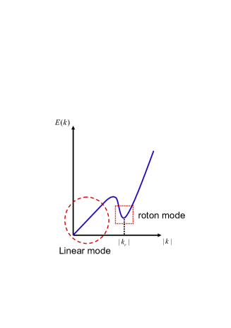
Figure 4: The spectrum of the quasi-particle in exciton BEC where there exist the linear mode and roton mode. This spectrum only holds when teh lifetime of the exciton $\tau_{ex}\rightarrow\infty$. The spectrum will be changed to Fig.6b when $\tau_{ex}$ is large, but finite.

IV The coherent state, line width and power spectrum in the normal direction at $\vec{k}=0$.

Because the condensate carries no in-plane momentum $\vec{k}=0$, so from $H_{int}^{c}$ in Eqn.24, the Heisenberg equation of motion of the photon annihilation operator is

$$i\partial_{t}a_{k_{z}}=(\omega_{k_{z}}-\mu-i\kappa)a_{k_{z}}-ig^{\ast}(k_{z})\sqrt{N}+iF(t)$$ (26)

where we have dropped the zero mode fluctuation of the zero momentum condensate which is negligible in the thermodynamic limit. The $\kappa$ is the decay rate of the photon due to its coupling to a reservoir ( or bath ), its value and physical meaning will be determined self-consistently in the following. The $F(t)$ is the fluctuation of the reservoir satisfying $\left\langle b\right|F(t)\left|b\right\rangle=0$ where $\left\langle O\right\rangle_{b}=Tr(\rho_{b}O)$ denotes the mean value of the operator $O$ at the bath state and $\rho_{b}$ is the density matrix of bath. From Eqn.26, one can see the exciton condensation $\sqrt{N}$ plays the role of an effective pump on the photon part. As shown in the Eqn.12, $g(k_{z})\sim L^{-1/2}_{z}$.

Following the standard laser theory, we decompose the operator as its mean plus its fluctuation: $a_{k_{z}}=\left\langle a_{k_{z}}\right\rangle_{in}+\delta a_{k_{z}}$ where the initial state $\left|{}\right\rangle_{in}$ in Fig.2 is taken to be $\left|BEC\right\rangle\left|0\right\rangle_{ph}\left|b\right\rangle$. Here, $\left|BEC\right\rangle$ denotes the ground state of the condensation; the initial photon state $\left|0\right\rangle_{ph}$ satisfies $a_{k_{z}}(0)\left|0\right\rangle_{ph}=0$ where $a_{k_{z}}(0)$ is the photon operator $a_{k_{z}}$ at the initial time $t=0$; $\left|b\right\rangle$ denotes the state of the photon reservoir. From Eqn.26, it is easy to see that

$$i\partial_{t}\left\langle a_{k_{z}}\right\rangle=(\omega_{k_{z}}-\mu-i\kappa)\left\langle a_{k_{z}}\right\rangle-ig^{\ast}(k_{z})\sqrt{N}.$$ (27)

The stationary solution is

$$\left\langle a_{k_{z}}\right\rangle=\frac{ig^{\ast}(k_{z})\sqrt{N}}{(\omega_{k_{z}}-\mu-i\kappa)}$$ (28)

which is the photon condensation induced by the exciton condensation at $\vec{k}=0$. So the output state along the normal direction is a coherent state.

The fluctuation $\delta a_{k_{z}}$ obeys:

$$i\partial_{t}\delta a_{k_{z}}=(\omega_{k_{z}}-\mu-i\kappa)\delta a_{k_{z}}+iF(t),$$ (29)

When $t>>1/\kappa$, the photon fluctuation is completely determined by the fluctuations of the reservoir:

$$\delta a_{k_{z}}(t)=\int_{0}^{t}d\tau F(\tau)e^{-i(\omega_{k_{z}}-\mu)(t-\tau)-\kappa(t-\tau)}.$$ (30)

Where the fluctuation-dissipation relation dictates that $\left\langle F^{\dagger}(t)F(t^{\prime})\right\rangle=\kappa\bar{n}_{\omega_{k_{z}}}\delta(t-t^{\prime}),\left\langle F(t)F^{\dagger}(t^{\prime})\right\rangle=\kappa(\bar{n}_{\omega_{k_{z}}}+1)\delta(t-t^{\prime}),\left\langle F(t)F(t^{\prime})\right\rangle=\left\langle F^{\dagger}(t)F^{\dagger}(t^{\prime})\right\rangle=0$.

From Eqn.30, we find:

$$\left\langle\delta a_{k_{z}}^{\dagger}(t)\delta a_{k_{z}}(t^{\prime})\right\rangle=\frac{1}{2}\bar{n}_{k_{z}}e^{-\kappa\left|t-t^{\prime}\right|}e^{i(\omega_{k_{z}}-\mu)(t-t^{\prime})}$$ (31)

The power spectrum of the fluctuation is given by the Fourier transformation of the correlation function:

$$S(\omega)=\int_{-\infty}^{+\infty}\left\langle\delta a_{k_{z}}^{\dagger}(t)\delta a_{k_{z}}(t^{\prime})\right\rangle e^{-i(\omega-\mu)(t-t^{\prime})}dt$$ (32)

where we have defined the photon frequency with respect to the chemical potential $\mu$.

By inserting Eqn. 31 into Eqn.32, we get and the power spectrum

$$S(\omega)=\frac{1}{2}\frac{\bar{n}_{\omega_{k_{z}}}\kappa}{(\omega-\omega_{k_{z}})^{2}+\kappa^{2}},$$ (33)

where the particle distribution of the photon reservoir is $\bar{n}_{\omega}=1/(e^{\omega/T}-1)$ and $T$ is the temperature of the reservoir. The result Eqn.33 is consistent with the Wiener-Khintchine theorem.

The number of the emitted photon is

$$n_{\omega_{k_{z}}}=\left\langle a_{k_{z}}^{\dagger}a_{k_{z}}\right\rangle=\frac{N\left|g(\mu/c)\right|^{2}}{(\omega_{k_{z}}-\mu)^{2}+\kappa^{2}}+\bar{n}_{\omega_{k_{z}}}/2,$$ (34)

where we have set $g^{\ast}(k_{z})$ around $\omega_{k_{z}}=\mu$. Because the condensate $N$ is much larger than the particle distribution of the bath $\bar{n}_{\omega_{k_{z}}}$, so when the temperature of the reservoir $T\rightarrow 0$ which is the case considered in this paper, the number of the emitted photon is dominated by the first term.

Now we will determine the value of $\kappa$ self-consistently. The total number of photons is

$$N_{ph}=\sum_{k_{z}}n_{\omega_{k_{z}}}=N(|g|^{2}D)/\kappa$$ (35)

where $D=L_{z}/v_{g}$ is the photon density of states at $\vec{k}=0$. Note that the exciton decay rate $\gamma_{0}=|g|^{2}D$ at $\vec{k}=0$ is independent of $L_{z}$ ( see Eqn. 44 and 48 for general expressions of the density of state $D_{\vec{k}}(\omega_{k})$ and the exciton decay rate $\gamma_{\vec{k}}$ at any $\vec{k}$ ). The $N_{ph}$ has to be proportional to $L_{z}$ in order to get a finite photon density in a given volume $L^{2}\times L_{z}$ in a stationary state. This self-consistency condition sets $\kappa=v_{g}/L_{z}\rightarrow 0$ so that

$$N_{ph}=N\gamma_{0}L_{z}/v_{g}\sim L_{z}$$ (36)

Plugging this value of $\kappa$ into Eqn.34 leads to:

$$n_{\omega_{k_{z}}}=N\gamma_{0}\delta(\omega_{k_{z}}-\mu)$$ (37)

which is independent of $L_{z}$ as required ! We showed that the power spectrum emitted from the exciton condensate has zero width. This conclusion is robust and is independent of any macroscopic details such as how photons are coupled to reservoirs.

The radiation rate from the condensate is:

$$P^{rd}_{0}=N\gamma_{0}\mu$$ (38)

which is also independent of $L_{z}$ as required. In fact, in the limit $\kappa=v_{g}/L_{z}\rightarrow 0$, Eqns. 33 becomes $S(\omega)=\bar{n}_{\omega_{k_{z}}}\delta(\omega-\omega_{k_{z}})$ which is negligible at low temperature. From the Eqn.27, one can see that both the pumping term $ig^{*}\sqrt{N}\sim L^{-1/2}_{z}$ and the dumping term $i\kappa\sim L^{-1}_{z}$ approach zero as $L_{z}\rightarrow\infty$ limit in such a way that a stationary state is reached.

From the experimental data in section IX, taking $N\sim 10^{5},\gamma_{0}\sim 0.1\mu eV,\mu\sim 1.54eV$, we find $P^{rd}_{0}\sim 1\mu W$.

In summary, the coherent light emitted from the condensate has the following remarkable properties: (1) highly directional: along the normal direction (1) highly monochromatic: pinned at a single energy given by the chemical potential $\mu$ (3) high power: proportional to the total number of excitons. These remarkable properties are independent of any microscopic details as such as the excitation power $P_{ex}$ and the line width of the pumping laser as long as they can generate excitons across the band gap. This fact could be useful to build highly powerful opto-electronic device. In the appendix D, we will give a more intuitive derivation of these results from a golden rule calculation.

V The input-output formalism for a stationary state at $\vec{k}\neq 0$

In this section, we consider the photons with in-plane momentum $\vec{k}\neq 0$. From Eqn.25, it is easy to see that due to the in-plane momentum conservation, the exciton with a fixed in-plane momentum $\vec{k}$ coupled to 3 dimensional photons with the same $\vec{k}$, but with different momenta $k_{z}$ along the $z$-direction, so we can view these photon acting as the bath of the exciton by defining $\Gamma_{\vec{k}}=\sum_{k_{z}}g(k)a_{k}$. As shown in Eqn.23, due to the dipole-dipole repulsion, even at $T=0$, there are also excitons depleted from the condensate. These excitons will emit photons at non-zero $\vec{k}$. By using the standard input-output formalism for a stationary state discussed in book1 , we will achieve the squeezed spectrum, angle resolved power spectrum and photon correlation functions of the emitted photon in the following sections.

The Heisenberg equations of motions of the photons and excitons are

$$\partial_{t}a_{k} = -i(\omega_{k}-\mu)a_{k}-g^{\ast}(k)\tilde{b}_{\vec{k}},$$

$$\partial_{t}B_{\vec{k}} = -i\Sigma B_{\vec{k}}+A_{\vec{k}},$$ (39)

where $B_{\vec{k}}=(\tilde{b}_{\vec{k}},\tilde{b}_{-\vec{k}}^{\dagger})^{T}$, $A_{\vec{k}}=(\Gamma_{\vec{k}},\Gamma_{-\vec{k}}^{\dagger})^{T}$ and

$$\Sigma=\left(\begin{array}[]{cc}\epsilon_{\vec{k}}+\bar{n}V_{d}(\vec{k})&\bar{n}V_{d}(\vec{k})\\ -\bar{n}V_{d}(\vec{k})&-\epsilon_{\vec{k}}-\bar{n}V_{d}(\vec{k})\end{array}\right).$$ (40)

The formal solution of $a_{k}$ can be written either as the initial state at $t_{0}<t$ or the final state at $t_{1}>t$:

$$a_{k}(t) = a_{k}(t_{0})e^{-i(\omega_{k}-\mu)(t-t_{0})}$$ (41)

$$-g^{\ast}(k)\int_{t_{0}}^{t}dt^{\prime}\tilde{b}_{\vec{k}}(t^{\prime})e^{-i(\omega_{k}-\mu)(t-t^{\prime})}$$

and

$$a_{k}(t) = a_{k}(t_{1})e^{-i(\omega_{k}-\mu)(t-t_{1})}$$ (42)

$$+g^{\ast}(k)\int_{t}^{t_{1}}dt^{\prime}\tilde{b}_{\vec{k}}(t^{\prime})e^{-i(\omega_{k}-\mu)(t-t^{\prime})},$$

When plugging Eqns. 41 and 42 into Eqn.39, we find it is convenient to define the input and output fields as:

$$a_{\vec{k}}^{in}(t) = \sum_{k_{z}}\frac{1}{\sqrt{D_{\vec{k}}(\omega_{k})}}a_{k}(t_{0})e^{-i(\omega_{k}-\mu)(t-t_{0})},$$

$$a_{\vec{k}}^{out}(t) = -\sum_{k_{z}}\frac{1}{\sqrt{D_{\vec{k}}(\omega_{k})}}a_{k}(t_{1})e^{-i(\omega_{k}-\mu)(t-t_{1})},$$ (43)

where the density of states of the photon with a given in-plane momentum $\vec{k}$ is

$$D_{\vec{k}}(\omega_{k})=\frac{\omega_{k}L_{z}}{v_{g}\sqrt{\omega_{k}^{2}-v_{g}^{2}\left|\vec{k}\right|^{2}}}$$ (44)

which is proportional to $L_{z}$. It can be shown that if $v_{g}|\vec{k}|\ll\mu$, the input and output fields obey the Bose commutation relations:

$$[a_{\vec{k}}^{in}(t),a_{\vec{k}^{\prime}}^{in\dagger}(t^{\prime})]=[a_{\vec{k}}^{out}(t),a_{\vec{k}^{\prime}}^{out\dagger}(t^{\prime})]=\delta_{\vec{k},\vec{k}^{\prime}}\delta(t-t^{\prime})$$ (45)

In term of the input field $\mathbf{a}_{\vec{k}}^{in}(t)=(a_{\vec{k}}^{in}(t),a_{-\vec{k}}^{in\dagger}(t))^{T}$, the exciton operator $B_{k}$ obeys

$$\partial_{t}B_{\vec{k}}=(-i\Sigma-\frac{\gamma_{\vec{k}}}{2})B_{\vec{k}}+\sqrt{\gamma_{\vec{k}}}\mathbf{a}_{\vec{k}}^{in},$$ (46)

In terms of the output field $\mathbf{a}_{\vec{k}}^{out}(t)=(a_{\vec{k}}^{out}(t),a_{-\vec{k}}^{out\dagger}(t))^{T}$, it obeys

$$\partial_{t}B_{\vec{k}}=(-i\Sigma+\frac{\gamma_{\vec{k}}}{2})B_{\vec{k}}-\sqrt{\gamma_{\vec{k}}}\mathbf{a}_{\vec{k}}^{out},$$ (47)

where the effects of photon-exciton coupling are completely encoded in the exciton decay rate $\gamma_{\vec{k}}=D_{\vec{k}}(\mu)\left|g_{\vec{k}}(\omega_{k}=\mu)\right|^{2}$:

$$\gamma_{\vec{k}}=\frac{E_{\vec{k}}^{ex2}\left|D_{k}\right|^{2}\sin^{2}\theta_{k}\phi^{2}(0)}{2\epsilon v_{g}(\mu^{2}-v_{g}^{2}\left|\vec{k}\right|^{2})^{1/2}},$$ (48)

where $\theta_{k}$ is the angle between the transition dipole moment $\vec{D}_{k}$ and the 3 dimensional photon vector $k$ shown in Fig.1b. Note that $\gamma_{\vec{k}}$ is independent $L_{z}$, so is an experimentally measurable quantity as shown in section IX-1. From the rotational invariance in the Fig.1b, we can conclude that $\gamma_{\vec{k}}\sim const.+|\vec{k}|^{2}$ as $\vec{k}\rightarrow 0$ as shown in Fig.6..

When comparing Eqn.46 and 47 with Eqn.26, we can see that input photon field $\sqrt{\gamma_{\vec{k}}}\mathbf{a}_{\vec{k}}^{in}$ ( or the output photon field $\sqrt{\gamma_{\vec{k}}}\mathbf{a}_{\vec{k}}^{out}$ ) which are summation of continuous spectral of photons at a given in-plane momentum $\vec{k}$, but with different $k_{z}$ as shown in Eqn.43 plays the role of the reservoir $F(t)$ for the excitons, while the exciton decay rate $\gamma_{\vec{k}}$ due to the photon-exciton coupling plays the role of $\kappa$. However, there is no similar source ( or pumping ) term like $-ig^{*}(k_{z})\sqrt{N}$.

When deriving Eqn.46 and 47, we have assumed the density of state $D_{\vec{k}}(\omega_{k})$ at a given in-plane momentum $\vec{k}$ varies slowly around the characteristic frequency $\omega_{k}=\mu$. Indeed as shown later in Figs.7.8.10, the maximum of squeezing spectrum and power spectrum is very narrowly peaked around $\omega_{k}=\mu$, so it is reasonable to set $\omega_{k}=\mu$ in $D_{\vec{k}}(\omega_{k})$. This approximation is essentially a Markov approximation which is valid only when the in-plane momentum $\left|\vec{k}\right|$ is much smaller than $\mu/v_{g}$ in Eqn.48. In fact, as to be shown in section VI-1, the maximum in-plane momentum $\left|\vec{k}_{max}\right|=\mu/v_{g}$. This is also the same approximation for the commutation relations Eqn.45 hold. However, when the emitted photon is along the plane, namely with $k_{z}=0$, the Markov approximation becomes in-valid. So all our following calculations are valid as long as the emitted photons are not too close to along the $xy$ plane.

The relation

$$\mathbf{a}_{\vec{k}}^{in}+\mathbf{a}_{\vec{k}}^{out}=\sqrt{\gamma_{\vec{k}}}B_{\vec{k}},$$ (49)

is derived from Eqn.46 and Eqn.47. The Fourier transformations of Eq. (46), Eq. (47) and Eq. (49) lead to input-output relation:

$$\mathbf{a}_{\vec{k}}^{out}(\omega)=W^{-1}(\omega)W^{\ast}(\omega)\mathbf{a}_{\vec{k}}^{in}(\omega)$$ (50)

where $W(\omega)=-\gamma_{\vec{k}}I/2+i(\omega I-\Sigma)$ and $\mathbf{a}_{\vec{k}}^{out}(\omega)$ and $\mathbf{a}_{\vec{k}}^{in}(\omega)$ are the Fourier transformation of $\mathbf{a}_{\vec{k}}^{out}(t)$ and $\mathbf{a}_{\vec{k}}^{in}(t)$. Then the component $a_{\vec{k}}^{out}(\omega)$ of the output field $\mathbf{a}_{\vec{k}}^{out}(\omega)$ is related to the input fields by:

$$a_{\vec{k}}^{out}(\omega) = [-1+\gamma_{\vec{k}}G_{n}(\vec{k},\omega+i\frac{\gamma_{k}}{2})]a_{\vec{k}}^{in}(\omega)$$ (51)

$$+\gamma_{\vec{k}}G_{a}(\vec{k},\omega+i\frac{\gamma_{k}}{2})a_{-\vec{k}}^{in\dagger}(-\omega),$$

where the normal Green function $G_{n}(\vec{k},\omega)$ and the anomalous Green function $G_{a}(\vec{k},\omega)$ are

$$G_{n}(\vec{k},\omega) = i\frac{\omega+\epsilon_{\vec{k}}+\bar{n}V_{d}(\vec{k})}{\omega^{2}-E^{2}(\vec{k})},$$

$$G_{a}(\vec{k},\omega) = \frac{i\bar{n}V_{d}(\vec{k})}{\omega^{2}-E^{2}(\vec{k})},$$ (52)

which are determined by the properties of the quasi-particle in the exciton BEC. In fact, they are just the retarded Green functions after making the analytic continuation $i\omega_{n}\rightarrow\omega+i\delta$ in the corresponding imaginary time Green functions. The exciton decay rate $\gamma_{\vec{k}}$ in the two Green functions in Eqn.51 just stand for the fact that the excitons are decaying into photons. Note that the Fourier transformation of the Eq. (43) leads to

$$\omega=\omega_{k}-\mu$$ (53)

In fact, Eqn.51 can be viewed as a $S$ matrix relating the input photon field at $t_{0}\rightarrow-\infty$ to the output photon field at $t_{1}\rightarrow\infty$. In the following sections, we will calculate the squeezed spectrum, angle resolved power spectrum and photon correlation functions of the emitted photons respectively..

VI Two mode Squeezing spectrum with $\vec{k}\neq 0$

Eqn. 51 suggests that the output field is the two mode squeezed state between $\vec{k}$ and $-\vec{k}$, so it is convenient to define $A_{\vec{k},\pm}^{out}(\omega)=[a_{\vec{k}}^{out}(\omega)\pm a_{-\vec{k}}^{out}(\omega)]/\sqrt{2}$ and $A_{\vec{k},\pm}^{in}(\omega)=[a_{\vec{k}}^{in}(\omega)\pm a_{-\vec{k}}^{in}(\omega)]/\sqrt{2}$. Then:

$$A_{\vec{k},\pm}^{out}(\omega) = [-1+\gamma_{\vec{k}}G_{n}(\vec{k},\omega+i\frac{\gamma_{k}}{2})]A_{\vec{k},\pm}^{in}(\omega)$$ (54)

$$\pm\gamma_{\vec{k}}G_{a}(\vec{k},\omega+i\frac{\gamma_{k}}{2})A_{\vec{k},\pm}^{in\dagger}(-\omega)$$

The position and momentum ( quadrature phase ) operators of the output field is defined by

$$X_{\pm} = A_{\vec{k},\pm}^{out}(\omega)e^{i\phi_{\pm}(\omega)}+A_{\vec{k},\pm}^{out\dagger}(-\omega)e^{-i\phi_{\pm}(-\omega)}$$

$$iY_{\pm} = A_{\vec{k},\pm}^{out}(\omega)e^{i\phi_{\pm}(\omega)}-A_{\vec{k},\pm}^{out\dagger}(-\omega)e^{-i\phi_{\pm}(-\omega)}$$ (55)

The squeezing spectra book1 which measure the fluctuation of the canonical position and momentum are defined by

$$S_{\vec{k},X_{\pm}}(\omega) = \left\langle X_{\pm}(\omega)X_{\pm}(-\omega)\right\rangle_{in},$$

$$S_{\vec{k},Y_{\pm}}(\omega) = \left\langle Y_{\pm}(\omega)Y_{\pm}(-\omega)\right\rangle_{in}.$$ (56)

where the $\delta(\omega+\omega^{\prime})$ function was omitted for notational simplicity, the in-state is the vacuum state of the input field $|BEC\rangle|0\rangle$ shown in Fig.4. Because the average $\left\langle X_{\pm}(\omega)\right\rangle_{in}=\left\langle Y_{\pm}(\omega)\right\rangle_{in}=0$, then the squeezing spectrums are $S_{X_{\pm}}(\omega)=|\Delta X_{\pm}(\omega)|^{2}$ and $S_{Y_{\pm}}(\omega)=|\Delta Y_{\pm}(\omega)|^{2}$. It can be shown that

$$S_{\vec{k},X_{\pm}}(\omega) = 1+\left\langle:X_{\pm}(\omega)X_{\pm}(-\omega):\right\rangle_{in},$$

$$S_{\vec{k},Y_{\pm}}(\omega) = 1+\left\langle:Y_{\pm}(\omega)Y_{\pm}(-\omega):\right\rangle_{in}.$$ (57)

where $:AB:$ denotes the normal order of the $A$ and $B$ with respect to the $A_{\vec{k},\pm}^{out}(\omega)$, but the average is taken with the incoming vacuum state.

For notational conveniences, we set $\phi_{-}(\omega)=\pi/2+\phi_{+}(\omega)$ and just set $\phi_{+}(\omega)\equiv\phi(\omega)$. Then we find $S_{X_{+}}(\omega)=S_{X_{-}}(\omega)=S_{X}(\omega)$ and $S_{Y_{+}}(\omega)=S_{Y_{-}}(\omega)=S_{Y}(\omega)$. The phase $\phi(\omega)$ in the Fig.5 is chosen to achieve the largest possible squeezing, namely, by setting $\partial S_{X}(\omega)/\partial\omega=0$ which leads to:

$$\cos 2\phi(\omega)=\frac{\gamma_{\vec{k}}(\epsilon_{\vec{k}}+\bar{n}V_{d}(\vec{k}))}{\sqrt{\Omega^{2}(\omega)+\gamma_{\vec{k}}^{2}E^{2}(\vec{k})+(\bar{n}V_{d}(\vec{k})\gamma_{\vec{k}})^{2}}},$$ (58)

where $\Omega(\omega)=\omega^{2}-E^{2}(\vec{k})+\gamma_{\vec{k}}^{2}/4$, the $\epsilon_{\vec{k}}$ and $E(\vec{k})$ are related by Eqn.21.

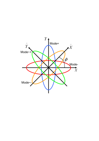
Figure 5: The two mode squeezed state in the quadrature phase space. Only when the photon frequency resonates with the quasi-particle energy at $E(\vec{k})>\gamma_{k}/2$, the two mode squeezed states are mode + and mode -. All the other cases have non-zero squeezing angles shown as mode $\tilde{}\pm$. See also Fig.9.

Substituting Eqns.51,54 and 55 into Eq. (56) leads to

$$S_{X}(\omega) = 1-\frac{2\gamma_{\vec{k}}\bar{n}V_{d}(\vec{k})}{\mathcal{N}(\omega)+\gamma_{\vec{k}}\bar{n}V_{d}(\vec{k})}$$

$$S_{Y}(\omega) = 1+\frac{2\gamma_{\vec{k}}\bar{n}V_{d}(\vec{k})}{\mathcal{N}(\omega)-\gamma_{\vec{k}}\bar{n}V_{d}(\vec{k})}$$ (59)

where $\mathcal{N}(\omega)=\sqrt{\Omega^{2}(\omega)+\gamma_{\vec{k}}^{2}E^{2}(\vec{k})+(\bar{n}V_{d}(\vec{k})\gamma_{\vec{k}})^{2}}$

Obviously:

$$S_{X}(\omega)S_{Y}(\omega)=\Delta X_{\pm}\Delta Y_{\pm}=1$$ (60)

The results show that for a given in-plane momentum $\vec{k}$ and a given individual photon frequency $\omega$ with respect to the chemical potential $\mu$, there always exists a two mode squeezing state which can be decomposed into two squeezed states along two normal angles: one squeezed along the angle $\phi(\omega)$ and the other along the angle $\phi(\omega)+\pi/2$ in the quadrature phase space ($X,Y$) as shown in Fig.5.

In the following, we discuss two cases $|\vec{k}|<k^{\ast}$ and $|\vec{k}|>k^{\ast}$ respectively. For this purpose, we draw the exciton energy $E(\vec{k})$ and the decay rate $\gamma_{\vec{k}}/2$ in the same plot in Fig.6. When $|\vec{k}|<k^{\ast}$, the excitons decay very fast into photons, so they are not well defined quasi-particles. However, when $|\vec{k}|\gg k^{\ast}$, the excitons decay into photons very slowly, so they are well defined quasi-particles.

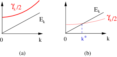
Figure 6: The energy spectrum and the decay rate of the exciton versus in-plane momentum $\vec{k}$. The direct exciton is always in case (a), the quasi-particles in Fig.4 are not well defined in any momentum scales. However, as argued in section IX, due to its large lifetime $\tau_{ex}$, the indirect exciton is in case (b). When $|\vec{k}|<k^{\ast}$, the quasi-particles in Fig.4 are not well defined . However, when $|\vec{k}|\gg k^{\ast}$, they are well defined quasi-particles. Compare with Fig.4 which is the case with $\tau_{ex}\rightarrow\infty$.

(1) Strong coupling case $|\vec{k}|<k^{\ast}$: $E(\vec{k})<\gamma_{\vec{k}}/2$.

From Eqn.59, we can see that the maximum squeezing happens at $\omega_{\min}=0$ which means at $\omega_{k}=\mu$:

$$S_{X}(\vec{k},\omega=0) = 1-\frac{2\gamma_{\vec{k}}\bar{n}V_{d}(\vec{k})}{\mathcal{N}(0)+\bar{n}V_{d}(\vec{k})\gamma_{\vec{k}}}$$

$$\cos 2\phi(\vec{k},\omega=0) = \frac{\gamma_{\vec{k}}(\epsilon_{\vec{k}}+\bar{n}V_{d}(\vec{k}))}{\mathcal{N}(0)}$$ (61)

where $\mathcal{N}(0)\equiv\mathcal{N}(\omega=0)=\sqrt{[E^{2}(\vec{k})+\gamma_{\vec{k}}^{2}/4]^{2}+(\bar{n}V_{d}(\vec{k})\gamma_{\vec{k}})^{2}}$which is defined below Eqn.59. In sharp contrast to the weak coupling case $E(\vec{k})>\gamma_{\vec{k}}/2$ to be discussed in the following, the resonance position $\omega_{k}=\mu$ is independent of the value of $\vec{k}$, this is because the quasiparticle is not even well defined in the strong coupling case. The $\omega$ dependence of $S_{X}(\omega)$ in Eqn.59 is drawn in Fig.7. The line width of the single peak in Fig. 7 is:

$$\delta_{1}(\vec{k})=2\sqrt{E^{2}(\vec{k})-\frac{\gamma_{\vec{k}}^{2}}{4}+O_{\vec{k}}},$$ (62)

where $O_{\vec{k}}=\sqrt{4\mathcal{N}(0)[\mathcal{N}(0)+\bar{n}V_{d}(\vec{k})\gamma_{\vec{k}}]-\gamma_{\vec{k}}^{2}E^{2}(\vec{k})}$.

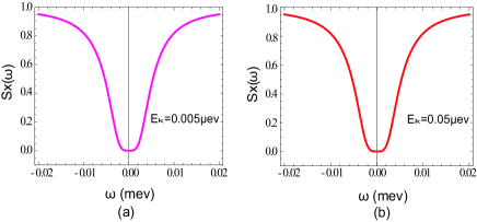
Figure 7: The squeezing spectrum at a given in-plane momentum $\vec{k}$ when $E(\vec{k})<\gamma_{\vec{k}}/2$. The $nV_{d}(\vec{k})$ and $\gamma_{\vec{k}}/2$ are fixed at $50\mu eV$ and $0.1\mu eV$ respectively as determined from experimental data in section IX. They are also used in the following figures 9,10,12-16. There exists only one minimal when the photon frequency equals to the chemical potential with the width $\delta_{1}(\vec{k})$ given by Eqn.62. Near the resonance, the squeezing ratio is so close to zero that it can not be distinguished in the figure. There are very little difference between the two energies $E(\vec{k})=0.005\mu eV$ and $E(\vec{k})=0.05\mu eV$. This is because the quasi-particles are not well defined in this case, the squeezing spectrum is mainly determined by $nV_{d}(\vec{k})$ and $\gamma_{\vec{k}}/2$.

(2) Weak coupling case $k>k^{\ast}$: $E(\vec{k})>\gamma_{\vec{k}}/2$.

As shown in Fig.6, in this case, $|\vec{k}|>k^{\ast}$. From Eqn.59, we can see that the maximum squeezing happens at the resonance frequency $\omega_{\min}=\pm[E^{2}(\vec{k})-\gamma_{\vec{k}}^{2}/4]^{1/2}$. Recall that the Fourier transformation of the Eq. (43) gives $\omega=\omega_{k}-\mu$, so the resonance condition becomes $\omega_{k}=\mu\pm[E^{2}(\vec{k})-\gamma_{\vec{k}}^{2}/4]^{1/2}$ where

$$S_{X}(\vec{k},\omega_{\min}) = (\frac{\epsilon_{\vec{k}}}{E(\vec{k})})^{2}=\frac{\hbar k^{2}}{\hbar^{2}k^{2}+4M\bar{n}V_{d}(\vec{k})}$$

$$\cos 2\phi(\vec{k},\omega_{\min}) = 1$$ (63)

In this case, $\phi(\vec{k},\omega_{\min})=0$, so the two squeezing modes are mode + and mode - respectively shown in Fig.5. In sharp contrast to the strong coupling case discussed above, the resonance positions depend on the value of $\vec{k}$, this is because the quasiparticle is well defined in the weak coupling case. The squeezing ratio is independent of $\gamma_{\vec{k}}$ at the resonances ! Of course, away from the resonances, it will always depends on $\gamma_{\vec{k}}$. From Eqn.63, we can see that increasing the exciton mass, the density and the exciton dipole interaction will all benefit the squeezing.

The $\omega$ dependence of $S_{X}(\omega)$ in Eqn.59 is drawn in Fig.8. When $E(\vec{k})>(Q_{\vec{k}}+\sqrt{1+Q_{\vec{k}}})\gamma_{\vec{k}}/2$, the line width of the each peak in Fig.8 is

$$\delta_{2}(\vec{k}) = \sqrt{E^{2}(\vec{k})-\frac{\gamma_{\vec{k}}^{2}}{4}+\gamma_{\vec{k}}Q_{\vec{k}}E(\vec{k})}$$

$$-\sqrt{E^{2}(\vec{k})-\frac{\gamma_{\vec{k}}^{2}}{4}-\gamma_{\vec{k}}Q_{\vec{k}}E(\vec{k})}$$

where $Q_{\vec{k}}=\sqrt{3+\frac{4\bar{n}V_{d}(\vec{k})}{\epsilon_{\vec{k}}}}$. It is easy to see that $\delta_{2}\sim\gamma_{\vec{k}}Q_{\vec{k}}$ which is equal to the exciton decay rate $\gamma_{\vec{k}}$ multiplied by a prefactor $Q_{\vec{k}}$.

When $E(\vec{k})<(Q_{\vec{k}}+\sqrt{1+Q_{\vec{k}}})\gamma_{\vec{k}}/2$, the two peaks are too close to be distinguished.

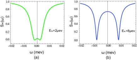
Figure 8: The squeezing spectrum at a given in-plane momentum $\vec{k}$ when $E(\vec{k})>\gamma_{\vec{k}}/2$. There exist two minima in the spectrum when the photon frequency resonate with the well defined quasi-particles. Near the resonance, the squeezing ratio is so close to zero that it can not be distinguished in the figure. When $E(\vec{k})=2\mu eV$, the two peaks are still not clearly separated. When $E(\vec{k})=8\mu eV\gg\gamma_{\vec{k}}/2$, the quasi-particles are well defined which lead to the two well defined resonances with width $\delta_{2}(\vec{k})$ in Eqn.VI.

In short, for a given in-plane momentum, there always exists a two mode squeezed state. When $E(\vec{k})<\gamma_{\vec{k}}/2$, the squeezing spectrum reaches its minimum Eq. 61 at $\omega_{k}=\mu$ and the squeezed angle is always non zero $\phi(\omega)\neq 0$. On the other hand, when $E(\vec{k})>\gamma_{\vec{k}}/2$, the squeezing spectrum reaches its minimum Eq. 63 at $\omega_{k}=\mu\pm[E^{2}(\vec{k})-\gamma_{\vec{k}}^{2}/4]^{1/2}$ and the squeezed angle $\phi(\omega_{\min})=0$. In sharp contrast to the widths in the ARPS and EDC in Fig.11,13 to be discussed in the Sec.VII which depend only on $\gamma_{\vec{k}}$, the two widths in Eqn.62 and VI in the squeezing spectra also depend on the interaction! The angle dependence of Eqn.58 in both the strong coupling $E(\vec{k})<\gamma_{\vec{k}}/2$ and the weak coupling $E(\vec{k})>\gamma_{\vec{k}}/2$ cases are drawn in the same plot Fig.9 for comparison. From Eq. 61 which is valid at $E(\vec{k})<\gamma_{\vec{k}}/2$ ( $|\vec{k}|<k^{\ast}$ ) and Eq. 63 which is valid at $E(\vec{k})>\gamma_{\vec{k}}/2$ ( $|\vec{k}|>k^{\ast}$ ) at the resonance, we can find that the squeezing ratio and the angle dependence at the resonance on the whole in-plane momentum $\vec{k}$ regime.

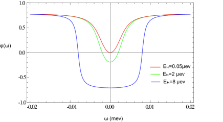
Figure 9: The squeezing angle dependence on the frequency when $E(\vec{k})<\gamma_{\vec{k}}/2$ and $E(\vec{k})>\gamma_{\vec{k}}/2$. When $E(\vec{k})<\gamma_{\vec{k}}/2$ the squeezing angle is always non-zero. Near the resonance, the angle is so close to zero that it can not be distinguished in the figure. Only when $E(\vec{k})>\gamma_{\vec{k}}/2$ and the photon frequency resonate with the well defined quasi-particles, the squeezing angle is zero. Away from the resonance, the angle becomes negative.

(3) Phase sensitive Homodyne measurement to measure the squeezing spectrum and the rotating phase $\phi(\omega)$

Usual measurements are just intensity measurement such as power spectrum experiment and intensity-intensity correlation measurement such as HBT experiment book1 ; book2 , so contain no phase information. Detection of squeezed states, on the other hand, requires a phase sensitive scheme that measures the variance of a quadrature of the photon field. This can be achieved the phase sensitive homodyne detection. The experimental set-up of this kind of experiment was explained in detail in book1 ; book2 , here we just briefly explain the main points of a single mode phase sensitive homodyne detection by a schematic Fig.10. This figure need to be connected with the homodyne outputs of the Fig.16 to detect the two modes squeezing spectrum Eqn.59 and squeezing angle Eqn.58. It is essentially a phase interference experiment between the input light beam A and a local oscillator (LO) beam B which is used as a reference beam. Both input beam A and LO beam B are incident on a beam splitter and are reflected and transmitted, there is a $\pi/2$ phase shift between the reflected and the transmitted beam. so there are two beams C and D coming out the splitter, both C and D are linear combination of A and B. If one fixed the LO beam B to be a strong coherent field with phase $\phi$, a balanced detection is to use a 50/50 beam splitter, the output signal detected by the coincidence measurement in the Fig.10 is taken to be the difference between the counting of C photons and that of D photons, so it is just the interference between the quadrature of the input beam A and the strong LO beam B subject to a rotation by angle $\phi+\pi/2$. The variance of the output can also be measured which is just the squeezing spectrum Eqn.56. By tuning the angle $\phi$, both $X$ quadrature and $Y$ quadrature or its any linear combination quadrature of the input beam can be measured. Then the rotated phase $\phi$ in Eqn.58 shown in Fig.5 and drawn in Fig.9 is just this phase $\phi$ of the local oscillator, so they are completely experimental measurable quantities in the phase sensitive homodyne experiments.

Figure 10: The balanced homodyne experiment to measure a single mode squeezing spectrum.

VII One photon correlation function, Power spectrum and Macroscopic super-radiance

The one photon correlation function of the output field is $G_{\pm}(\tau)=\left\langle a_{\pm\vec{k}}^{out\dagger}(t+\tau)a_{\pm\vec{k}}^{out}(t)\right\rangle_{in}$ and the angle resolved power spectrum (ARPS) of the output field is $S_{\pm}(\vec{k},\omega)=\int_{-\infty}^{+\infty}d\tau e^{-i\omega\tau}G_{\pm}(\tau)$. The normalized first order correlation function is defined by $g_{\pm}(\tau)=G_{\pm}(\tau)/G_{\pm}(0)$. In the following, we will evaluate these quantities respectively.

(1) The angle resolved power spectrum (ARPS)

By inserting Eqn.51, one obtains the photon number spectrum $S_{\pm}(\vec{k},\omega)=S_{1}(\vec{k},\omega)$ and

$$S_{1}(\vec{k},\omega) = \frac{1}{4}(S_{X}(\omega)+S_{Y}(\omega)-2)$$ (65)

$$= \frac{\gamma_{\vec{k}}^{2}\bar{n}^{2}V_{d}^{2}(\vec{k})}{\Omega^{2}(\omega)+\gamma_{\vec{k}}^{2}E^{2}(\vec{k})}.$$

where $\Omega(\omega)=\omega^{2}-E^{2}(\vec{k})+\gamma_{\vec{k}}^{2}/4$. From Eqn.60, one can see that $S_{X}(\omega)+S_{Y}(\omega)\geq 1$, so the more squeezing, the stronger the power spectrum. If there is no squeezing $S_{X}(\omega)=S_{Y}(\omega)=1$, then there is no power emitted, this is just the input vacuum state in the Fig.4 which is a coherent state itself. The angle resolved power spectra (ARPS) with different $E(\vec{k})$ and $\gamma_{\vec{k}}$ are shown in Fig.11. The total ARPS is the sum of the condensate and the quasi-particles: $S(\vec{k},\omega)=S_{0}(\vec{k},\omega)+S_{1}(\vec{k},\omega)$.

In the strong coupling case $k<k^{*},E(\vec{k})<\gamma_{\vec{k}}/2$, $S_{1}(\vec{k},\omega)$ reaches the maximum $\gamma_{\vec{k}}^{2}\bar{n}^{2}V_{d}^{2}(\vec{k})/[\gamma_{\vec{k}}^{2}/4+E^{2}(\vec{k})]^{2}$ at $\omega_{k}=\mu$. As $\vec{k}\rightarrow 0$, $E(\vec{k})=u|\vec{k}|\rightarrow 0$, then $S_{1}(\vec{k},\omega)\rightarrow\frac{\gamma_{\vec{k}}^{2}\bar{n}^{2}V_{d}^{2}(\vec{k})}{(\omega^{2}+\gamma_{\vec{k}}^{2}/4)^{2}}$, so the curve has a half width $\sim\hbar\gamma_{0}\sim 10^{-4}meV$. This is expected, because the quasiparticles are not well defined with the decay rate $\gamma_{0}$ much larger than its energy $E(\vec{k})$.

In the weak coupling case $E(\vec{k})>\gamma_{\vec{k}}/2$, at the two resonance frequencies $\omega_{k}=\mu\pm[E^{2}(\vec{k})-\gamma_{\vec{k}}^{2}/4]^{1/2}$, $S_{1}(\vec{k},\omega)$ reaches the maximum $\bar{n}^{2}V_{d}^{2}(\vec{k})/E^{2}(\vec{k})$ which only depends on the exciton density, the dipole-dipole interaction and the quasi-particle spectrum, but independent of $\gamma_{\vec{k}}$ ! It can be shown that when $E(\vec{k})\gg\gamma_{\vec{k}}/2$, the width of the two peaks at the two resonance frequencies is $\sim\gamma_{\vec{k}}$, this is expected, because the quasi-particle is well defined with energy $[E^{2}(\vec{k})-\gamma_{\vec{k}}^{2}/4]^{1/2}$ and the half-width $\gamma_{\vec{k}}$. In sharp contrast to the two widths in Eqn.62 and VI in the squeezing spectra which depend on both the interaction and $\gamma_{\vec{k}}$, the widths in the ARPS and EDC in Fig.11,13 depend only on $\gamma_{\vec{k}}$.

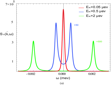
Figure 11: The angle resolved power spectrum (ARPS) of the emitted photon with in-plane momentum $\vec{k}$. When $E(\vec{k})\leq\hbar\gamma_{\vec{k}}/2$, there is only one peak in the power spectrum with the width $\gamma_{\vec{k}}/2$. When $E(\vec{k})>\hbar\gamma_{\vec{k}}/2$, there are two peaks in the power spectrum at the two resonance photon frequencies $\omega_{k}\simeq\mu\pm E(\vec{k})$ also with width $\gamma_{\vec{k}}/2$. The $S_{1}(\vec{k},\omega)$ at $E(\vec{k})=0.5\mu eV$ and $E(\vec{k})=2\mu eV$ are multiplied by $50$ and $500$ in order to be seen in the figure. Compared to the squeezing spectrum in Fig.9, one can see the ARPS can distinguish the two quasi-particle peaks clearly even at $E(\vec{k})=0.5\mu eV$. While the squeezing spectrum in Fig.9 can not distinguish the two quasi-particle peaks even at $E(\vec{k})=2\mu eV$, so the ARPS is a much sensitive probe of the quasi-particle spectrum than the squeezing spectrum.

(2) Momentum Distribution Curve (MDC)

The power spectrum at a given in-plane momentum $\vec{k}$ is $S_{1}(\vec{k})=\sum_{k_{z}}S_{1}(\vec{k},\omega)=\int d\omega_{k}D_{\vec{k}}(\omega_{k})S_{1}(\vec{k},\omega)$ which is nothing but the Momentum Distribution Curve (MDC) myprl :

$$S_{1}(\vec{k})=\frac{D_{\vec{k}}(\mu)\bar{n}^{2}V_{d}^{2}(\vec{k})\gamma_{\vec{k}}}{2[E^{2}(\vec{k})+(\frac{\gamma_{\vec{k}}}{2})^{2}]}\propto L_{z}$$ (66)

As to be explained in section IX and shown in the Fig.6, the crossing point is at $k^{\ast}\sim 10^{-2}cm^{-1}$. From Eqn.36, one can see the condensate contribution at $\vec{k}=0$ is $N_{ph}/L_{z}=N\gamma_{0}/v_{g}\propto N$, while the contribution from the quasi-particle is $S_{1}(\vec{k}\rightarrow 0)/L_{z}=\frac{2n^{2}V^{2}_{d}(0)}{v_{g}\gamma_{0}}\propto n^{2}/\gamma_{0}$. So the MDC is a Lorentian with the half width at $k^{\ast}$ as shown in the Fig.12. So the $k^{\ast}$ has a clear physical meaning as the half width of the MDC and is an experimentally measurable quantity.

In fact, we can also calculate the one photon correlation function:

$$G(r)\sim\int\frac{d^{2}\vec{k}}{(2\pi)^{2}}\frac{e^{i\vec{k}\cdot\vec{r}}}{k^{2}+k^{*2}}\sim e^{-k^{*}r}$$ (67)

where we can identify the coherence length $\xi\sim 1/k^{*}\sim 40\mu m$. This coherence length has been measured in coherence and will be discussed in detail in section IX.

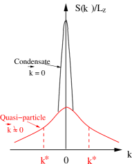
Figure 12: The zero temperature Momentum Distribution Curve (MDC) has a bi-model structure consisting of a sharp peak $S(\vec{k}=0)/L_{z}=N\gamma_{0}/v_{g}$ due to the condensate at $\vec{k}=0$ superposing on a Lorentzian peak with a half width $k^{\ast}\sim 10^{2}cm^{-1}$ due to quasi-particle excitations at $\vec{k}\neq 0$. The coherence $\xi\sim 1/k^{*}$ has been measured in coherence .

(3) Energy Distribution Curve (EDC)

The power spectrum at a given energy $\omega$ is $S_{1}(\omega)=\sum_{\vec{k}}S_{1}(\vec{k},\omega)$ which is nothing but the Energy Distribution Curve (EDC)myprl :

$$S_{1}(\omega) = N\bar{n}\times\int\frac{d^{2}\vec{k}}{(2\pi)^{2}}\frac{\gamma_{\vec{k}}^{2}V_{d}^{2}(\vec{k})}{\Omega^{2}(\omega)+\gamma_{\vec{k}}^{2}E^{2}(\vec{k})}$$ (68)

$$= \frac{N\bar{n}V^{2}_{d}(\vec{k}=0)}{4\pi u^{2}}f(\frac{|\omega|}{\gamma_{\vec{k}=0}})\propto N\bar{n}$$

where $f(x)=\frac{1}{x}[\frac{\pi}{2}-arctg\frac{1/4-x^{2}}{x}]$ where $-\pi/2<arctgy<\pi/2$. Because $f(0)=4$, then $S_{1}(\omega=0)/N=\frac{\bar{n}V^{2}_{d}(\vec{k}=0)}{\pi u^{2}}$. The $S_{1}(\omega)$ is shown in Fig.13a.

The $S_{1}(\omega)$ is the sum over all the angle resolved power spectrum curves in Fig.11 at the fixed energy $\omega=\omega_{k}-\mu$. As $\vec{k}\rightarrow 0$, $E(\vec{k})=u|\vec{k}|\rightarrow 0$, then $S_{1}(\vec{k},\omega)\rightarrow\frac{\gamma_{\vec{k}}^{2}\bar{n}^{2}V_{d}^{2}(\vec{k})}{(\omega^{2}+\gamma_{\vec{k}}^{2}/4)^{2}}$, so the curve has a half width $\sim\hbar\gamma_{0}\sim 10^{-4}meV$. As $|\vec{k}|$ increases to $k^{*}\sim 10^{-2}cm^{-1}$, the curve starts to split into two peaks as shown in the Fig.11, then when $|\vec{k}|\rightarrow|\vec{k}_{max}|/2$, the two peaks stand for the two well defined quasi-particle excitations, the splitting of the two peaks reaches $\sim u|\vec{k}_{max}|\sim 0.1meV$. So the EDC curve will simply smear out all the fine structures of the angle resolved power spectrum in Fig.11 and finally end up with an envelop curve with a half width $w_{e}\sim\gamma_{\vec{k}}$ as shown in the Fig.13. From Eqn.37, one can see the condensate contribution at $\vec{k}=0$ is $n_{\omega_{k_{z}}}/N=\gamma_{0}\delta(\omega_{k_{z}}-\mu)$, while the contribution from the quasi-particle $S_{1}(\omega=0)/N=\frac{\bar{n}V^{2}_{d}(\vec{k})}{\pi u^{2}}$ as shown in the Fig.13a. As to be explained in section IX, the EDC is what experiments in butov ; snoke measured at various $P_{ex},V_{g}$ and $T$.

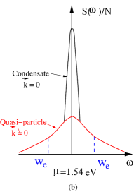
Figure 13: (a) The Energy Distribution Curve ( EDC ) from the quasi-particle. (b) The zero temperature EDC has a bi-model structure consisting of a sharp $\delta$ function peak $S(\omega)/N=\gamma_{0}\delta(\omega-\mu)$ due to the condensate at $\vec{k}=0$ superposing on a Lorentzian peak with the half envelop width $w_{e}\sim\gamma_{\vec{k}}\sim 0.1\mu eV$ due to quasi-particle excitations at $\vec{k}\neq 0$.

(4) The total radiation rate from the quasi-particles

The total number of photons emitted from the quasi-particles is:

$$S_{1}=\sum_{k_{z}}\sum_{\vec{k}}S_{1}(\vec{k},\omega)\sim N\times L_{z}\bar{n}$$ (69)

which is proportional to the total normalization volume of the system as it is expected. This can also be used as a self-consistency check on our results achieved on the quasi-particle part at $\vec{k}\neq 0$. As shown in the section IV, this self-consistency check played very important roles on the condensate part $\vec{k}=0$. In fact, if taking Eqns.68 and 66 at face value, then the total number of photons Eqn.69 diverge, but this should not cause any concern, because both Eqns.68 and 66 only hold at small momentum $k<k_{max}$ and $\omega<uk_{max}$ respectively.

The radiation rate along a given direction $(\vec{k},k_{z})$ is:

$$P^{ra}_{1}(\vec{k},k_{z})=\frac{S_{1}(\vec{k},\omega)}{L^{2}L_{z}}\omega_{k}v_{g}\times L^{2}$$ (70)

which vanishes in the limit $L_{z}\rightarrow\infty$ as expected. Then the radiation rate at a given in-plane momentum $P^{ra}_{1}(\vec{k})=v_{g}\mu S_{1}(\vec{k})/L_{z}$ and the radiation rate at a given energy $P^{ra}_{1}(\omega)=v_{g}\mu S_{1}(\omega)/L_{z}$ where we have used the fact that $S_{1}(\vec{k},\omega)$ is a even function of $\omega=\omega_{k}-\mu$.

The total radiation rate from the quasi-particles is:

$$P^{ra}_{1}=\sum_{k_{z}}\sum_{\vec{k}}P_{rd}(\vec{k},k_{z})=v_{g}\mu S_{1}/L_{z}\propto v_{g}\mu N\bar{n}$$ (71)

where again $k_{z}$ is sum over both the upper and the lower space in the Fig.1b. $P^{ra}_{1}$ is also $\propto\mu N$ just as the radiation rate $P^{ra}_{0}$ from the condensate. Because of the weak dipole-dipole interaction, the quantum depletion is small, so $P^{ra}_{1}$ is still much smaller than $P^{ra}_{0}$ in Eqn.38. Furthermore $P^{ra}_{1}$ is spread over all the possible angles, while $P^{ra}_{0}$ is focused along a single direction.

(5) One photon correlation functions

By using the Fourier transformation to $S_{1}(\vec{k},\omega)$, one can get $G_{\pm}(\vec{k},\tau)=G_{1}(\vec{k},\tau)$

$$G_{1}(\vec{k},\tau)=\frac{\bar{n}^{2}V_{d}^{2}(k)\gamma_{k}}{4E(k)}[\frac{e^{i(E(k)+i\frac{\gamma_{k}}{2})\tau}}{E(k)+i\frac{\gamma_{k}}{2}}+h.c.],$$ (72)

The normalized first order correlation function $g_{\pm}(\vec{k},\tau)=g_{1}(\vec{k},\tau)$, where

$$g_{1}(\vec{k},\tau)=e^{-\frac{\gamma_{\vec{k}}}{2}\tau}[\cos(E(\vec{k})\tau)+\frac{\gamma_{\vec{k}}}{2E(\vec{k})}\sin(E(\vec{k})\tau)]$$ (73)

It turns out that the first order correlation function is independent of the relation between $E(\vec{k})$ and $\gamma_{\vec{k}}/2$ and is shown in Fig.14. The $G_{1}$ was measured in the EHBL in coherence at $T=1.6K$ and in exciton polariton in exp2 at $T=4K$. The effects of finite temperature and trap potential must be considered before comparing our theoretical results with the experimental data.

Figure 14: The one photon correlation function

(6) The quasi-particle spectrum in a non-equilibrium stationary exciton superfluid

It is important to compare the excitation spectrum in Fig.4, Fig.6a and Fig.6b. Fig.4 is the well know quasi-particle excitations in an equilibrium superfluid. They are well defined quasi-particles with infinite lifetime. However, the quasi-particles in Fig.6a are not well defined in any length scales, because the decay rate is always much larger than the energy. Fig.6(b) is between the two extreme cases. When $k<k^{*}$, the quasi-particle is not well defined, the ARPS is centered around $\omega_{k}=\mu$ with the width $\gamma_{k}$. The MDC has large values at $k<k^{*}$. The EDC has large values at $\omega<\gamma_{k}$. When $k>k^{*}$, the quasi-particles is well defined, the ARPS has two well defined quasi-particles peaks at $\omega_{k}=\mu\pm[E^{2}(\vec{k})-\gamma_{\vec{k}}^{2}/4]^{1/2}$ with the width $\gamma_{k}$. The MDC has very small values at $k>k^{*}$. The EDC has very small values at $\omega>\gamma_{k}$. So in the long wavelength $r>\xi\sim 1/k^{*}$ ( or small momentum $k<k^{*}$ ) limit and long time $\tau>\tau_{ex}\sim 1/\gamma_{k}$ (or low energy limit $\omega<\gamma_{k}$ ) limit, there is not a well defined superfluid which is consistent with the results achived in kohn . However, in the distance sacle $r<\xi\sim 1/k^{*}$ ( or momentum $k>k^{*}$ ) limit and the time scale $\tau<\tau_{ex}\sim 1/\gamma_{k}$ (or energy scale $\omega>\gamma_{k}$ ), there is still defined superfluid and associated quasi-particle excitations. This is the main difference and analogy between the equilibrium superfluid in Fig.4 and the non-equilibrium steady state superfluid in Fig.6b. Very recently, the elementary excitation spectrum of exciton-polariton inside a micro-cavity was measured expp and was found to be very similar to that in a helium 4 superfluid shown in Fig.4 except in a small regime near $k=0$. We believe this observation is precisely due to the excitation spectrum in a non-equilibrium stationary superfluid shown in Fig.6b.

(7) The Superradiance from the quasi-particles

Note that the angle resolved power spectrum, the MDC and EDC in Eqns.65 66, 68 are all proportional to $N^{2}$ instead of $N$. It is the characteristic of super-radiance in a macroscopic system. This should not be too surprising, because the excitonic superfluid is a macroscopic quantum coherence phenomena, so it is natural to lead to macroscopic superradiance. As $k\rightarrow 0$ in the Fig.6, $S_{1}(\vec{k})\sim\frac{\bar{n}^{2}V^{2}_{d}(k)}{\gamma_{\vec{k}}}\sim\bar{n}^{2}/\gamma_{\vec{k}}$ where $\gamma_{k}$ appears in the denominator in the strong coupling case, so the macroscopic superradiance can only be achieved by the non-perturbative calculations presented in this section, but can not be derived by any finite order perturbative calculations presented in the appendix D.

In conventional quantum optics, $N$ two level atoms interacting with a single ( or multi-) photon mode(s) inside a cavity. If the $N$ static atoms are confined into a small volume $V$ inside the cavity which is much smaller than the wavelength of the photon mode, then the interaction between all the $N$ atoms and the photon mode can be taken as the same constant $\lambda$, then when half of the atoms are in the excited level, the radiation intensity from the $N$ atoms is proportional to $N^{2}$ instead of just $N$ during the time interval $\sim 1/N$, so the total power emitted during this time period is $N^{2}\times 1/N\sim N$ as required by the energy conservation. This is due to the cooperative effects of the $N$ atoms which is due to the fact that the $N$ atoms, being interacting with the same photon field, so can not be treated as independent $N$ atoms. This is called non-equilibrium superradiance first studied by Dicke super . Generalizing the Dicke model to a stationary state inside a cavity was studied in dick1 ; dick2 . It was found that there is a second order phase transition driving the coupling constant $\lambda$: when $\lambda<\lambda_{c}$, the system is in a normal phase, when $\lambda>\lambda_{c}$, the system is in a superradiative phase. It was also pointed out in dick2 that it is very unrealistic to realize Dicke model in the thermodynamic limit $N,V\rightarrow\infty$, but keep $N/V$ to be finite, because it is essentially impossible to make $V$ still smaller than the wavelength of the photon in the thermodynamic limit. So the superradiance is essentially an effect for finite number of static atoms confined into a small volume.

The superradiance from the ESF has completely different mechanism: (1) the size of the sample is much larger than the wavelength of the photon field (2) The photons field is a continuum of photons with different $k_{z}$ at a given $\vec{k}$ in Eqn.15, so acting as a reservoir to the excitons with in-plane momentum $\vec{k}$ (3) all the excitons are always in motion, in fact, moving in a coherent fashion. So all these conditions violate the conditions to achieve the superradiance in conventional quantum optics. So the collective radiation from the ESF is due to the macroscopic coherence of the exciton superfluid itself which is, in turn, due to the dipole-dipole repulsion.

VIII Two photon correlation functions and photon statistics

The quantum statistic properties of emitted photons can be extracted from two photon correlation functions. The normalized second order correlation functions of the output field for the two modes at $\vec{k}$ and $-\vec{k}$ are

$$g_{2}^{(\vec{k})}(\tau)=\frac{\left\langle a_{\vec{k}}^{out\dagger}(t)a_{\vec{k}}^{out\dagger}(t+\tau)a_{\vec{k}}^{out}(t+\tau)a_{\vec{k}}^{out}(t)\right\rangle_{in}}{\left|G_{1}(0)\right|^{2}}$$ (74)

and

$$g_{2}^{(\pm\vec{k})}(\tau)=\frac{\left\langle a_{\vec{k}}^{out\dagger}(t+\tau)a_{\vec{k}}^{out}(t+\tau)a_{-\vec{k}}^{out\dagger}(t)a_{-\vec{k}}^{out}(t)\right\rangle_{in}}{\left|G_{1}(0)\right|^{2}}$$ (75)

The second order correlation function $g_{2}^{(\pm\vec{k})}(\tau)$ determines the probability of detecting $n_{-\vec{k}}$ photons with momentum $-\vec{k}$ at time $t$ and detecting $n_{\vec{k}}$ photons with momentum $\vec{k}$ at time $t+\tau$. Just like the one photon correlation function in Eqn.73, it turns out that the second correlation functions are also independent of the relation between $E(\vec{k})$ and $\gamma_{\vec{k}}/2$ and are shown in Fig.15. The Wick theorem foot gives $g_{2}^{(\vec{k})}(\tau)=1+\left|g_{1}(\tau)\right|^{2}$ where $g_{1}(\tau)$ is given by Eqn.73. Similarly, it can be shown that $g_{2}^{(\pm\vec{k})}(\tau)=1+\left|f_{1}(\tau)\right|^{2}$ where

$$f_{1}(\tau) = -\frac{E^{2}(\vec{k})+\frac{\gamma_{\vec{k}}^{2}}{4}}{\bar{n}V_{d}(\vec{k})}e^{-\frac{\gamma_{\vec{k}}}{2}\tau}$$ (76)

$$\times [u_{\vec{k}}^{2}\frac{e^{-iE(\vec{k})\tau}}{E(\vec{k})-i\frac{\gamma_{\vec{k}}}{2}}+v_{\vec{k}}^{2}\frac{e^{iE(\vec{k})\tau}}{E(\vec{k})+i\frac{\gamma_{\vec{k}}}{2}}].$$

Then the normalized second order correlation functions are

$$g_{2}^{(\vec{k})}(\tau)=1+e^{-\gamma_{\vec{k}}\tau}[\cos(E(\vec{k})\tau)+\frac{\gamma_{\vec{k}}}{2E(\vec{k})}\sin(E(\vec{k})\tau)]^{2}$$ (77)

and

$$g_{2}^{(\pm\vec{k})}(\tau) = 1+e^{-\gamma_{\vec{k}}\tau}\{\frac{E^{2}(\vec{k})+\frac{\gamma_{\vec{k}}^{2}}{4}}{\bar{n}^{2}V_{d}^{2}(k)}$$ (78)

$$+[\cos(E(\vec{k})\tau)+\frac{\gamma_{\vec{k}}}{2E(\vec{k})}\sin(E(\vec{k})\tau)]^{2}\}$$

It is easy to see that the envelope decaying function is given by the exciton decay rate $\gamma_{\vec{k}}$, while the oscillation within the envelope function is given by the Bogoliubov quasi-particle energy $E(\vec{k})$. Subtracting Eqn.78 from Eqn.77 lead to:

$$g_{2}^{(\pm\vec{k})}(\tau)-g_{2}^{(\vec{k})}(\tau)=e^{-\gamma_{\vec{k}}\tau}\frac{E^{2}(\vec{k})+\frac{\gamma_{\vec{k}}^{2}}{4}}{\bar{n}^{2}V_{d}^{2}(k)}$$ (79)

So we only draw $g_{2}^{(\pm\vec{k})}(\tau)$ in the Fig.18.

Figure 15: The two photon correlation functions between $\vec{k}$ and $-\vec{k}$ against the delay time $\tau$. The envelope of second order correlation function decreases as time evolves indicates that the emitted photons is photon bunching and the photo-count statistics is super-Poissonian.

When $\tau=0$ the two photon correlation function are $g_{2}^{(\vec{k})}(0)=2$, so just the mode $\vec{k}$ alone behaves like a chaotic light. This is expected because the entanglement is only between $-\vec{k}$ and $\vec{k}$. In fact,

$$g_{2}^{(\pm k)}(0)=2+\frac{E^{2}(\vec{k})+\frac{\gamma_{\vec{k}}^{2}}{4}}{\bar{n}^{2}V_{d}^{2}(\vec{k})}>g_{2}^{(\vec{k})}(0)=2.$$ (80)

So it violates the classical Cauchy-Schwarz inequality which is completely due to the quantum nature of the two mode squeezing between $\vec{k}$ and $-\vec{k}$.

The normalized two photon correlation function $g_{2}^{(\pm\vec{k})}(\tau)$ is shown in Fig. 15. From Fig. 15, we can find that the two photon correlation functions decrease as time interval $\tau$ increases which suggests quantum nature of the emitted photons is photon bunching and the photo-count statistics is super-Poissonian. See Fig.17 for its experimental measurement.

IX Discussions on available experimental data and possible future experiments

We will determine how all the important parameters in our theory can be precisely measured by the experiments. Then we will compare our results on the EDC with the available experimental data butov ; snoke and then discuss possible future experimental set-ups to detect all the other theoretical predictions achieved in the previous sections.

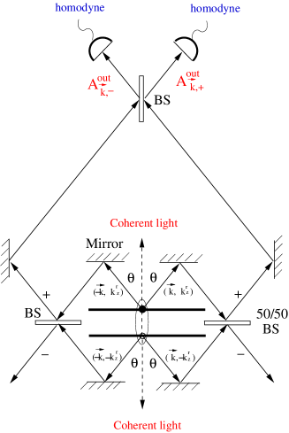
Figure 16: The experimental set-up for the homodyne detection of the two modes squeezed photon in the EHBL system. The coherent photons are emitted along the z-direction reflecting the nature of the condensation. The squeezed photons are emitted along all the tilted directions reflecting the fluctuation above the condensation. There is a macroscopic superradiance when the angle $\theta$ is small. The homodyne coming out of $A^{out}_{\vec{k},+}$ or $A^{out}_{\vec{k},-}$ is connected to Fig.10 for the single mode squeezing spectrum measurement.

1. Comments on current experimental data

In butov ; snoke , the spatially and spectrally resolved photoluminescence intensity has a sharp peak at the emitted photon energy $E=1.545eV$ with a width $\sim 1meV$ at the lowest temperature $\sim 1K\sim 0.1meV$. The radiation power $P_{ex}$ varies from $17\mu W$ to $1.6mW$. The gate voltage is set at $V_{g}=1.2V$. As shown in Eqn.16, one can identify $E=\mu=E_{g}-E_{b}+\bar{n}V_{d}(0)=1.545eV$. The energy conservation at $k_{z}=0$ gives the maximum in-plane momentum $\vec{k}_{max}\sim\mu/v_{g}\sim 4.3\times 10^{4}cm^{-1}$ where we used the speed of the light $v_{g}\simeq 8.7\times 10^{9}cm/s$ in $GaAs$ butov . Then the maximum exciton energy $E_{max}=uk_{max}\sim 0.15meV$ where we used the spin wave velocity $u\sim 5\times 10^{5}cm/s$. Taking the mass of the exciton $M\sim 0.22m_{0}$ butov , then from the expression of the spin wave velocity $u=\sqrt{\bar{n}V_{d}(0)/M}$ calculated in Eqn.22, we find $\bar{n}V_{d}(0)\simeq 0.05meV$ which is the value we used in all the previous Figs.7-15. Taking the exciton density $n\sim 10^{10}cm^{-2}$, we can see that $K=2\pi/a\sim 10^{6}cm^{-1}$ where $a$ is the average spacing between excitons. The average lifetime of the indirect excitons in the EHBL butov ; snoke is $\tau_{ex}\sim 40ns$, then we can estimate the exciton decay rate $\gamma_{k}\sim 1/40ns\sim 10^{-4}meV=0.1\mu ev$. At the boundary of the two regimes in the Fig.6 where $E(k^{\ast})=uk^{\ast}=\gamma_{k^{\ast}}/2=10^{-4}meV$, we can extract $k^{\ast}=2.4\times 10^{2}cm^{-1}$. So there are three widely separated momentum scales, $k^{\ast}\sim 10^{2}cm^{-1}\ll k_{max}\sim 10^{4}cm^{-1}\ll K\sim 10^{6}cm^{-1}\sim k_{r}$ which is the roton minimum in Fig.4. So all the important parameters such as the chemical potential $\mu$, the quasi-particle energy $E(\vec{k})=u|\vec{k}|$, the exciton decay rate $\gamma_{\vec{k}}$ and the exciton dipole-dipole interaction strength $\bar{n}V_{d}(0)$ in our theory can all be extracted from experimental data.

The typical trap size ( or exciton cloud size ) $L\sim 30\mu m$. The number of excitons is $N=nL^{2}\sim 10^{5}$ which is comparable to the number of cold atoms inside a trap in most cold atom experiments. The central peak due to the condensate in the MDC Fig.12 is broadened to $k_{0}\sim 1/L\sim 10^{3}cm^{-1}$ which is already larger than the half width due to the quasi-particle $k^{\ast}\sim 10^{-2}cm^{-1}$. So it is impossible to distinguish the bi-model structure in the MDC at such a small exciton size. The coherence length was measured in coherence . From Eqn.67, we find the coherence $\xi\sim 1/k^{*}\sim 40\mu m$ which is slightly larger than the exciton cloud size $L\sim 30\mu m$.

For an inhomogeneous condensate $\langle b(\vec{k})\rangle=\psi(\vec{k})$ inside a harmonic trap $V(r)=\frac{1}{2}ur^{2}$, we assume local density approximation (LDA) is valid, then Eqn.26 should be replaced by:

$$i\partial_{t}a(\vec{k},k_{z})=(\omega(\vec{k},k_{z})-\mu+V(r)-i\kappa)a(\vec{k},k_{z})-ig^{\ast}(\vec{k},k_{z})\psi(\vec{k})$$ (81)

where we have still dropped the zero mode fluctuation of the inhomogeneous condensate. Because $g^{\ast}(\vec{k},k_{z})\sim L^{-1/2}_{z}\rightarrow 0$ and $\kappa=v_{g}/L_{z}\rightarrow 0$ such that a stationary state is reached where the energy $\omega(\vec{k},k_{z})$ is pinned at the local chemical potential $\mu(r)=\mu-V(r)$, so the central peak due to the condensate in the EDC in the Fig.13a is broadened simply due to the change of the local chemical potential from the center to the edge of the trap $\Delta\omega=\frac{1}{2}uL^{2}\sim 0.1meV$ where we used the experimental value butov ; snoke $u\sim 10^{-12}eVnm^{-2}$. This geometrical broadening due to the trap is already much larger than the half width due to the quasi-particle $w_{e}\sim\gamma_{\vec{k}}\sim 0.1\mu eV$ in Fig.13b, so it is impossible to distiguish the bi-modal structure in the EDC in the Fig.13b. In order to understand if the observed EDC peak with the width $\sim 1meV$ at the lowest temperature $\sim 1.7K$ in the experiments in butov ; snoke is indeed due to the exciton condensate, one has to study how the bi-model structures shown in Fig.13b will change inside a harmonic trap at a finite temperature $\sim 1.7K$ and the effects of both dark and bright excitons. This will be discussed in a separate publication diffusion .

2. Possible future angle resolved experiments

As shown in section VII, the MDC, especially the EDC smear out all the fine structures of the angle resolved power spectrum in the Fig.11. So in order to test the theoretical results precisely, it is necessary to perform the ARPS measurement. As one rotates the angle $\tan\theta_{k}=\left|\vec{k}/k_{z}\right|$ of the photo-detector in the Fig.1b, one should see the following interesting behaviors. When $|\vec{k}|<|\vec{k}^{\ast}|$, the ARPS and the squeezing spectrum only have one peak at the resonance frequency $\omega_{k}=\mu\sim 1.545eV$ as shown in Fig.11, Fig.7 and Fig.18b. The line width of the peak is uniquely determined by the quasi-particle excitation $u\left|\vec{k}\right|$ and the decay rate $\gamma_{\vec{k}}$. The one peak will start to split into the two peaks at $u\left|\vec{k}^{\ast}\right|\mathbf{=}\gamma_{\vec{k}^{\ast}}/2$ corresponding to the angle $\sin\theta^{*}=k^{*}/k_{max}\sim 10^{-2}$, so $\theta^{*}\sim 10^{-2}$. When $\vec{k}>\vec{k}^{\ast}$ ( namely, $\theta>\theta^{*}$ ), both the ARPS and the squeezing spectrum have two peaks at the two resonance frequencies $\omega_{k}=v_{g}(k_{z}^{2}+\vec{k}^{2})^{1/2}=1.545eV\pm[u^{2}\left|\vec{k}\right|^{2}-\gamma_{\vec{k}}^{2}/4]^{1/2}$ as shown in Fig.11, Fig.8 and and Fig.18b. The position and the width of the two peaks are uniquely determined by the quasi-particle excitation $uk$ and the decay rate $\gamma_{\vec{k}}$. So all the characters of the condensate and the fluctuations above it are reflected in the angle resolved measurements of squeezing spectrum and the power spectrum.

3. Possible future two modes phase sensitive homodyne experiments

As shown in the appendix C, due to the relation Eqn.93, the experimental set-up in Fig.16 combined with the single mode phase sensitive homedyne set-up in Fig.10 can measure the squeezing spectrum in Eqn.59 and the squeezing angle in Eqn.58.

4. Possible future two modes HanburyBrown-Twiss type of experiments

The single mode two photon correlation functions $g^{(\vec{k})}_{2}(\tau)$ in Eqn.74 can be measured by the usual HBT set-up book1 ; book2 . It is not very interesting anyway. From the relation in Eqn.89, we can see the experimental set-up in Fig.17 can measure the most interesting two modes two photon correlation functions $g^{(\pm\vec{k})}_{2}(\tau)$ in Eqn.78 and Fig.15.

Figure 17: HanburyBrown-Twiss ( HBT ) type of experiment to measure the two modes two photon correlation functions $g^{(\pm\vec{k})}_{2}(\tau)$ in Eqn.78 and Fig.15.

X Conclusions

In conventional quantum optics, coherent light was produced by stimulated radiations from a pump which leads to particle number inversion and amplified by optical resonator, here in EHBL, the coherent state along the normal direction is due to a complete different and new mechanism: spontaneous symmetry breaking. It has the following remarkable properties: (1) highly directional: along the normal direction (1) highly monochromatic: pinned at a single energy given by the chemical potential $\mu$ (3) high power: proportional to the total number of excitons. These remarkable properties could be useful to build highly powerful opto-electronic device.

In conventional non-linear quantum optics, the generation of squeezed lights also requires an action of a strong classical pump and a large non-linear susceptibility $\chi^{(2)}$. The first observation of squeezed lights was achieved in non-degenerate four-wave mixing in atomic sodium in 1985 fourwave . Here in EHBL, the generation of the two mode squeezed photon is due to a complete different and new mechanism: the anomalous Green function of Bogoliubov quasiparticle which is non-zero only in the excitonic superfluid state. The results achieved in this paper are robust against any microscopic details. The applications of the squeezed state include (1) the very high precision measurement by using the quadrature with reduced quantum fluctuations such as the $X$ quadrature in the Fig.2 and 3 where the squeeze factor reaches very close to $0$ at the resonances (2) the non-local quantum entanglement between the two twin photons at $\vec{k}$ and $-\vec{k}$ can be useful for many quantum information processes. (3) detection of possible gravitational waves grav .

In conventional quantum optics, $N$ non-interacting atoms confined in a small volume interact with photon modes, a super-radiance was proposed by Dicke. Very recently, there are preliminary experimental evidence that excitons in assembly of quantum dots may emit Dicke’s superradiance dots . In conventional laser, due to random motions of atoms confined in a volume larger than the wavelength of the laser beam, the laser power is only proportional to $N$ when the pump is above the threshold. So far, no super-radiant laser has been achieved. Here the ESF phase is a macroscopic quantum phenomena in a macroscopic sample ( namely in the thermodynamic limit ), so the super-radiance emitted from this system has completely different mechanism than the Dicke model.

In conventional quantum phase transitions, all the quantum phases and phase transitions are stable phases at equilibrium. For example, all the possible interesting quantum phases in BLQH mentioned in the introduction are stable equilibrium phases. However, the quantum phases in EHBL in Fig.3 are just meat-stable phases, they will eventually decay through emitting photons, photons are very natural internal probe of the quantum phases and quantum phase transitions. The characteristics of the photons such as power spectrum, squeezing spectrum and photon correlations are completely determined by the nature of the quantum phases such as the ground state and elementary excitations. The excitation spectrum in a non-equilibrium superfluid shown in Fig.6b is also different from that in a conventional equilibrium superfluid shown in Fig.6a. This difference completely and precisely explained the recent experimental observation of excitation spectrum of exciton-polariton in a planar microcavity expp .

In conventional condensed matter experiments, ground states are completely stable, so in order to externally probe the quasi-particle excitations of a quantum phases, the temperature to perform the experiments has to be sufficiently high so there are enough quasi-particle excitations excited above the ground state. However, the quantum phases in the Fig.3 are just meta-stable, so the internal probe of emitted photons from the quantum phase can also reflect the energy spectrum of the quasi-particle even at $T=0$. This is the salient feature of the internal probe in meta-stable systems different from the external probes in conventional stable condensed matter experiments. Exploring the connection between the quantum phase transitions and quantum optics in meta-stable non-equilibrium systems is still a developing field and very exciting and rich.

It is very instructive to compare the possible exciton BEC in EHBL with the well established BEC of ultra-cold atoms bloch . The quantum degeneracy temperature of two dimensional excitons can be estimated to be $T^{ex}_{d}\sim 3K$ for exciton density $n\sim 10^{10}cm^{-2}$ and effective exciton mass $m=0.22m_{e}$, so it can be reached easily by $He$ refrigerator. While due to the heavy mass of atoms and the dilute density, $T^{atom}_{d}\sim\mu K$. Both the exciton BEC and the atomic BEC belong to the weakly interacting BEC class, so Bogoliubov theory apply to both cases. The BEC to BCS crossover and quantum phases in Fig.3 tuned by $r_{s}$ or imbalance is also quite similar to those of two species of ultra-cold neutral fermions tuned by Feshbach resonance or imbalance bloch . In fact, atomic BEC is also a meta-stable ground state, it will eventually evaporate away. The conventional way to detect the atomic BEC is through the time of flight experiments which will destruct the BEC. The smoking gun experiment to prove the realization of BEC is through the observation of vortices when the BEC is under rotation. In this paper, we explicitly showed that although it is hard to rotate the metastable excitonic BEC to generate the superfluid vortices, the non-equilibrium stationary Bogoliubov quasi-particle spectrum of the exciton BEC in teh Fig.6b can be directly extracted from various characteristics of the emitted photons even at $T=0$. A superradiant behavior was found in the off-resonant light scattering experiment from the BEC condensate offscattering and studied theoretically in prltheory . In the off-resonant scattering, the excited atomic state is adiabatically eliminated, so important phase information containing the excitation spectrum is lost in the adiabatic elimination procedure. In the exciton BEC phase studied in this paper, the photons are always internally resonant with the excitons, so it becomes a complete natural internal probe of the ground state and excitations of all the possible exciton quantum phases. However, so far, there is very little experimental ways to measure the Bogoliubov quasi-particle of atomic BEC phononbec . So detecting quantum phases in ultracold atoms remains an outstanding problem. Recently, one of the authors and his collaborators developed a theory to detect the nature of quantum phases of ultra-cold atoms loaded on optical lattices by using cavity enhanced off-resonant light scattering jiangming . Excitons carry a electric dipole moment. While in the context of cold atoms, very exciting perspectives have been opened by recent experiments on cooling and trapping of ${}^{52}Cr$ cromium and polar molecules junpolar . Being electrically or magnetically polarized, the ${}^{52}Cr$ atoms or polar molecules interact with each other via long-rang anisotropic dipole-dipole interactions. The superfluid and solid phases of these polar molecules are under extensive experimental search junpolar ; polarroton . The excitation spectrum very similar to that in Fig. 3 including the roton minimum has also been proposed in trapped pancake dipolar Bose-Einstein condensates polarroton in atomic experiments. The presence, position and depth of the roton minimum are tunable by varying the density, confining potential. So the insights and results achieved in this paper may also shed some lights on cold atoms and molecules.

Before getting to the final summary of the results achieved in this paper, we briefly mention some previous and very recent work on semi-conductor electron-hole bilayers. BCS pairing of excitons and BEC to BCS crossover were discussed in cross1 ; cross2 . These mean field calculations can only describe the quasi-particle part, but contains no information on the collective modes. However, on the BEC side in the Fig.3 discussed in this paper, it is the collective mode shown in Fig.6b which contributes to the two mode squeezing state. Quantum Monte-carlo using trial-wavefunctions on the global phase diagram in Fig. 3 except the possible excitonic supersolid phase ye were studied in eh1 ; eh2 . The transport properties were studied in inplane , but we disagree with the claim made in inplane that an in-plane magnetic field can induce a counterflow supercurrent. The photoluminescence from the excitons inside a harmonic trap was studied by using first order Fermi Golden rules in golden by treating the exciton BEC as a single two level atom. This Golden rule treatment was not able to capture any of the physical phenomena explored in this paper which treat the exciton BEC as a quantum phase with its symmetry breaking ground state and Bogoliubov excitation spectrum. In the appendix D, we will use a first and second order Golden rule calculations which treat the exciton BEC as a quantum phase with a ground state and infinitely many excited states with different number of Bogoliubov quasi-particles. This kind of Golden calculation based on many particle ground and excited states can see some signatures of the results on coherent state and squeezed state achieved by non-perturbative calculations in the main context. The two phonon squeezing generated by lattice an-harmonic effects and second-order Raman scattering was discussed in phonon . As shown in section VII, the squeezing is closely related to the macroscopic superradiance, so it would be interesting to see if one can achieve a macroscopic super-radiance of phonons.

Several kinds of measurements such as angle resolved power spectrum, two mode squeezing spectrum, one photon and two photon correlations functions can completely detect the characters of the emitted photons which, in turn, are very natural internal probes of the ground state and excitations of exciton of the quantum phases in the EHBL system. We established the direct relation between the nature of quantum phases and the nature of the emitted photons from the quantum phases: the BEC of excitons lead to the coherent state ( or a spontaneous laser ) of emitted photons. The anomalous Green function of the Bogoliubov quasi-particles lead to the two mode squeezing of emitted photons along all the titled directions. The whole system behave coherently to emit superradiance even in the thermodynamic limit. In fact, the ESF phase of the excitons play a similar role as a two mode squeezing operator which squeezes the input vacuum state into a two mode squeezed state in a suitable rotated frame. We also evaluated the energy distribution curve (EDC) and momentum distribution curve (MDC) and compared our results with the available experimental data on MDC and EDC. We determined how all the important parameters such as the chemical potential $\mu$, the quasi-particle energy $E(\vec{k})=u|\vec{k}|$, the exciton decay rate $\gamma_{\vec{k}}$ and the exciton dipole-dipole interaction strength $\bar{n}V_{d}(0)$ in our theory can all be extracted from experimental data. The photons in all directions show bunching and super-Poissonian. Possible future angle resolved power spectrum experiments, two modes phase sensitive homodyne experiment to measure the squeezing spectrum, two modes HanburyBrown-Twiss experiment to measure the two photon correlation functions can be used to directly test these predictions. In fact, if the exciton BEC was indeed achieved in the past experiments butov ; snoke ; bell remains unclear. In future publications, we will study the effects of traps, spins of the excitons and finite temperature. The theoretical results achieved and possible future experimental set-up proposed in this paper should shed considerable lights to test if the exciton BEC can be observed in the EHBL without any ambiguities.

Acknowledgements

We are very grateful for Dr. Peng Zhang for helpful discussions. J.Ye is indebted to B. Halperin for critical reading of the manuscript and many critical suggestions. J. Ye is grateful for A. V. Balatsky, L. Butov, Jason Ho, Guoxinag Huang, Xuedong Hu, Allan Macdonald, Hui Deng, Zhibing Li, Qian Niu, Zhe-Yu Oh, Lu Sham, D. Snoke, Marc Ulrich, Hailing Wang, C. L Yang, Wang Yao, Xiaolu Yu, Fuchun Zhang, Keye Zhang, Weiping Zhang for helpful discussions. J. Ye’s research at KITP-C is supported by the Project of Knowledge Innovation Program (PKIP) of Chinese Academy of Sciences, at KITP was supported in part by the NSF under grant No. PHY-0551164.

Appendix A The physical pictures in terms of radiation zones

For simplicity, we first explain the physical picture at the zeroth order where we neglect the decay of excitons into photons in the Fig.18a. Note that at zero temperature $T=0$, there is no quasi-particle $\beta_{\vec{k}}$ excitation in Eqn.20, namely, the input state in the Fig.4. is the ground state $|BEC>$ ! However, what couples to the photons is $\tilde{b}_{\vec{k}}$ in Eqn.25 which is a linear combination of $\beta_{\vec{k}}$ and $\beta^{\dagger}_{\vec{k}}$. Equivalently, the phase $\theta$ fluctuation used in ye is a relativistic excitation which has both positive particle branch and negative energy anti-particle branch. The vacuum energy of the photon $E^{ph}_{0}$ is sitting below that of the exciton $E^{ex}_{0}$ by the chemical potential $\mu$, namely, $E^{ex}_{0}-E^{ph}_{0}=\mu$. There exists the resonance condition not only between the photon and the positive energy branch of the particle: $\hbar\omega_{k}=1.545eV+u\left|\vec{k}\right|$, but also between the photon and the negative energy branch of the anti-particle: $\hbar\omega_{k}=1.545eV-u\left|\vec{k}\right|$ as shown in Fig.18a.

When the effects of the excitons decaying into photons are taken into account self-consistently, the above picture need to be modified especially at small value of $\vec{k}$. When $|\vec{k}|<\vec{k}^{\ast}$, the two quasi-particle branches in Fig.18a are not well defined anymore, the power spectrum and the squeezing spectrum only have one peak at resonance frequency $\omega_{k}=\mu=1.545eV$. The one peak starts to split into two peaks at $u\left|\vec{k}^{\ast}\right|\mathbf{=}\gamma_{\vec{k}^{\ast}}/2$ where the quasi-particle excitations are still not well defined. However, when $|\vec{k}|\gg|\vec{k}^{\ast}|$, the two quasi-particle branches in the Fig.18a remain well defined, so both the power spectrum and the squeezing spectrum have two peaks at the resonance frequencies $\omega_{k}=v_{g}(k_{z}^{2}+\vec{k}^{2})^{1/2}=1.545eV\pm[u^{2}\left|\vec{k}\right|^{2}-\gamma_{\vec{k}}^{2}/4]^{1/2}$ as shown in Fig.18b. The flat regime in the Fig.18b precisely and completely explained the ” anomaly ” near $k=0$ of the excitation spectrum of exciton-polariton in a planar microcavity expp .

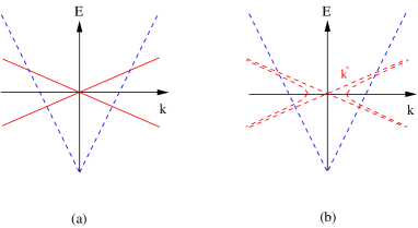
Figure 18: The radiative zone (RZ) in BEC ESF phase (a) The exciton lifetime $\tau_{ex}\rightarrow\infty$. The RZ is the regime of $E(\vec{k})$ between the four intersection points. (b) The exciton lifetime $\tau_{ex}$ is large, but finite. The solid gray parabola lines denote $\mu\pm[u^{2}\left|\vec{k}\right|^{2}-\gamma_{\vec{k}}^{2}/4]^{1/2}$ when $E(\vec{k})>\gamma_{\vec{k}}/2$, the blue dashed line denote $\omega_{k}=v_{g}\sqrt{\left|\vec{k}\right|^{2}+k^{2}_{z}}$ at $k_{z}=0$. When $E(\vec{k})<\gamma_{\vec{k}}/2$, intersection point between the dashed blue line and the horizontal axis leads to the maximum squeezing which is a two mode squeezed state, but with non-zero squeezing angle shown as $\tilde{\pm}$ in Fig.5. This horizontal axis leads to the the ” anomaly ” near $k=0$ of the excitation spectrum of exciton-polariton in a planar microcavity expp . When $E(\vec{k})>\gamma_{\vec{k}}/2$, the intersection points between the dashed blue line and the solid gray lines lead to the maximum squeezing which is a two mode squeezed states with zero squeezing angle shown as $\pm$ in Fig.5.

.

Appendix B The two mode squeezed state from a more intuitive view

In this appendix, we take a more intuitive way to show that no matter $E(\vec{k})<\gamma_{\vec{k}}/2$ or $E(\vec{k})>\gamma_{\vec{k}}/2$, the emitted photons are in a two mode squeezed state even off the resonance. This conclusion is very robust and independent of any microscopic details. This appendix supplement the more formal discussions in section VI.

The position and momentum ( quadrature phase ) operators of the output field can be more intuitively and straightforwardly defined as:

$$X_{\pm} = A_{\vec{k},\pm}^{out}(\omega)+A_{\vec{k},\pm}^{out\dagger}(-\omega),$$

$$Y_{\pm} = -i[A_{\vec{k},\pm}^{out}(\omega)-A_{\vec{k},\pm}^{out\dagger}(-\omega)].$$ (82)

The Eq. (51) and Eq. (56) give the relation $S_{\vec{k},X_{+}}(\omega)=S_{\vec{k},Y_{-}}(\omega)\equiv S_{X}(\omega)$ and $S_{\vec{k},Y_{+}}(\omega)=S_{\vec{k},X_{-}}(\omega)\equiv S_{Y}(\omega)$ and the squeezing spectra:

$$S_{X}(\omega) = 1-\frac{2\bar{n}V_{d}(\vec{k})\gamma_{\vec{k}}^{2}\epsilon_{\vec{k}}}{\Omega^{2}(\omega)+\gamma_{k}^{2}E^{2}(k)},$$

$$S_{Y}(\omega) = 1+\frac{2\bar{n}V_{d}(\vec{k})\gamma_{\vec{k}}^{2}(\epsilon_{\vec{k}}+2\bar{n}V_{d}(\vec{k}))}{\Omega^{2}(\omega)+\gamma_{\vec{k}}^{2}E^{2}(\vec{k})},$$ (83)

where $\Omega(\omega)=\omega^{2}-[E^{2}(\vec{k})-\gamma_{\vec{k}}^{2}/4]$.

The two variance functions are defined as book1 :

$$V_{\pm}(\omega)=<X_{\pm}(\omega)Y_{\pm}(-\omega)+Y_{\pm}(\omega)X_{\pm}(-\omega)>_{in}/2$$ (84)

From Eqn.51, we can determine:

$$V_{+}(\omega)=-V_{-}(\omega)=-\frac{2\gamma_{\vec{k}}\bar{n}V_{d}(\vec{k})[\omega^{2}-E^{2}(\vec{k})+\frac{\gamma_{k}^{2}}{4}]}{\Omega^{2}(\omega)+\gamma_{\vec{k}}^{2}E^{2}(\vec{k})}$$ (85)

From Eqn.83, we can find that:

$$S_{X}(\omega)S_{Y}(\omega)=1+\frac{\Omega^{2}(\omega)(2\bar{n}V_{d}(\vec{k})\gamma_{\vec{k}})^{2}}{[\Omega^{2}(\omega)+\gamma^{2}_{\vec{k}}E^{2}(\vec{k})]^{2}}\geq 1$$ (86)

which seems suggest that the state may not be a minimum uncertainty state. However, from Eqn.86 and Eqn.85, we can see that $\Delta X^{2}_{\pm}\Delta Y^{2}_{\pm}=1+|V_{\pm}|^{2}$ even off the resonance which indicates it is a two mode squeezed state if we can choose quadrature phase properly. From Eqn.83 and Eqn.85, we can see that if we define: $\tilde{X}_{\pm}+i\tilde{Y}_{\pm}=(X_{\pm}+iY_{\pm})e^{\pm i\phi}$ and choose squeezing parameter $\epsilon=re^{i2\phi}$ such that:

$$\cosh 2r = 1+\frac{2(\bar{n}V_{d}(\vec{k})\gamma_{\vec{k}})^{2}}{\Omega^{2}(\omega)+\gamma^{2}_{\vec{k}}E^{2}(\vec{k})},$$

$$\cos 2\phi = \frac{\gamma_{\vec{k}}(\epsilon_{\vec{k}}+\bar{n}V_{d}(\vec{k}))}{\sqrt{[\Omega^{2}(\omega)+\gamma^{2}_{\vec{k}}E^{2}(\vec{k})]+(\bar{n}V_{d}(\vec{k})\gamma_{\vec{k}})^{2}}}$$ (87)

Then we can show that $\tilde{S}_{X}=\Delta\tilde{X}^{2}_{\pm}=e^{-2r},\tilde{S}_{Y}=\Delta\tilde{Y}^{2}_{\pm}=e^{2r}$ and

$$\Delta\tilde{X}_{\pm}\Delta\tilde{Y}_{\pm}=1$$ (88)

which show that the emitted photons are still in the two mode squeezed state in the basis of $(\tilde{X}_{\pm},\tilde{Y}_{\pm})$ even off the resonance after making the rotation $\phi$ in the original basis $(X_{\pm},Y_{\pm})$ as shown in Fig.6. It is easy to see Eqn.87 is identical to Eqn.58 and Eqn.59.

Appendix C The relation between the calculated quantities and Experiment measurable quantities

Note that the emitted photons at time $t_{1}$ are described by the operator $a_{k}(t_{1})$ in Eqn.43, so it is necessary to find the relation between $a_{k}(t_{1})$ and $a^{out}_{\vec{k}}(\omega)$ through the Eq. (43). The Fourier transformation of Eq.43 leads to:

$$a_{\vec{k}}^{out}(\omega)=-\sum_{k_{z}}\frac{1}{\sqrt{D_{\vec{k}}(\omega+\mu)}}a_{k}(t_{1})e^{i\omega t_{1}}\delta(\omega_{k}-\mu-\omega)$$

$$=-\sqrt{D_{\vec{k}}(\omega+\mu)}e^{i\omega t_{1}}[a_{(\vec{k},k_{z}^{r})}(t_{1})+a_{(\vec{k},-k_{z}^{r})}(t_{1})]$$ (89)

where $k_{z}^{r}=[(\omega+\mu)^{2}/v^{2}_{g}-\left|\vec{k}\right|^{2}]^{1/2}$. So $a_{\vec{k}}^{out}(\omega)$ is a linear combination of $a_{(\vec{k},k_{z}^{r})}(t_{1})$ and $a_{(\vec{k},-k_{z}^{r})}(t_{1})$, both are at the output time $t_{1}$.

Then we can get:

$$\langle a^{\dagger}_{(\vec{k},k_{z})}(t_{1})a_{(\vec{k},k_{z}^{\prime})}(t_{1})\rangle=\langle a_{\vec{k}}^{\dagger out}(\omega)a_{\vec{k}}^{out}(\omega^{\prime})\rangle/D_{\vec{k}}(\mu)$$

$$=S_{1}(\vec{k},\omega)\delta(\omega-\omega^{\prime})/D_{\vec{k}}(\mu)$$ (90)

where, in fact, only $k_{z}^{\prime}=k_{z}$ contributes and $S_{1}(\vec{k},\omega)$ is given by Eqn.65. The total photon number at a given in-plane momentum $\vec{k}$ is :

$$\sum_{k_{z}}\sum_{k^{\prime}_{z}}\langle a^{\dagger}_{(\vec{k},k_{z})}(t_{1})a_{(\vec{k},k_{z}^{\prime})}(t_{1})\rangle$$

$$=\int d\omega_{k}D_{\vec{k}}(\omega_{k})S_{1}(\vec{k},\omega)=\sum_{k_{z}}S_{1}(\vec{k},\omega)$$ (91)

which is nothing but the momentum distribution curve in Eqn.66.

The total photon number at a given energy $\omega=v_{g}\sqrt{\vec{k}^{2}+k^{2}_{z}}$ is :

$$\sum_{\vec{k}}\sum_{k_{z}}\sum_{k^{\prime}_{z}}\delta_{k_{z},k^{\prime}_{z}}\langle a^{\dagger}_{(\vec{k},k_{z})}(t_{1})a_{(\vec{k},k_{z}^{\prime})}(t_{1})\rangle$$

$$=\sum_{\vec{k}}\sum_{k_{z}}S_{1}(\vec{k},\omega)\delta(\omega-\omega^{\prime})/D_{\vec{k}}(\mu)=\sum_{\vec{k}}S_{1}(\vec{k},\omega)$$ (92)

which is nothing but the energy distribution curve in Eqn.68.

A putative single mode squeezing spectrum of $a_{\vec{k}}^{out}(\omega)$ can be achieved by coincident detection of two photons both with in-plane momentum $\vec{k}$, but one with $z$-direction momenta $k_{z}$, the other with $-k_{z}$ shown in Fig.16. As shown in sect V-A, in fact, the squeezed state is a two mode squeezed state between $\vec{k}$ and $-\vec{k}$, so only the photons described by $A_{\vec{k},\pm}^{out}(\omega)=[a_{\vec{k}}^{out}(\omega)\pm a_{-\vec{k}}^{out}(\omega)]/\sqrt{2}=-\sqrt{D_{\vec{k}}(\omega+\mu)/2}e^{i\omega t_{1}}\tilde{A}_{\vec{k},\pm}^{out}(\omega)$ are in the squeezed state where

$$\tilde{A}_{\vec{k},\pm}^{out}(\omega) = [a_{(\vec{k},k_{z}^{r})}(t_{1})+a_{(\vec{k},-k_{z}^{r})}(t_{1})$$ (93)

$$\pm (a_{(-\vec{k},k_{z}^{r})}(t_{1})+a_{(-\vec{k},-k_{z}^{r})}(t_{1}))]$$

So the coincident detection experiment shown in Fig. 15 between the photons with momentum $(\vec{k},\pm k_{z}^{r})$ and $(-\vec{k},\pm k_{z}^{r})$ at the output time $t_{1}$ can lead to the squeezing spectrum $S_{X}(\vec{k},\omega)$ in Eqn.59. Just as the Markov approximation made in the section V, because the squeezing spectrum in Fig.7 and Fig.8 and power spectrum in Fig.11 are narrowly peaked at $\omega=0$ and $D_{\vec{k}}(\omega+\mu)$ is also a slowly varying function of $\omega$, so we can simply set $D_{\vec{k}}(\omega+\mu)\sim D_{\vec{k}}(\mu)$ as a constant prefactor at a given in-plane momentum $\vec{k}$ in the squeezing, power spectrum, macroscopic super-radiance and correlation function calculations in the section V. The photons described by $A_{\vec{k},-}^{out}(\omega)$ is squeezed along the direction normal to the squeezed direction of the photons described by $A_{\vec{k},+}^{out}(\omega)$ in the phase space as shown in Fig.5.

Appendix D Golden rule calculation to second order and two mode squeezed photons

This appendix was inspired by J.Ye’s visit to Univ. of Texas at Austin. J.Ye acknowledge very inspiring discussions with A. Macdonald, Qian Niu and Yao Wang. There are also independent unpublished work by Jung-Jung Su and A. Macdonald private . The input-output formalism used in the main text is to solve a integral-differential equation under the standard Markov approximation which is assuming the coupling constant varies little over the characteristic energy which is the exciton energy $\mu\sim 1.54ev$, this approximation is valid here. So the coupling constant $g_{k}$ was treated non-perturbatively under the Markov approximation in the main text. To reproduce the results achieved in this formalism by Golden rule is very diffucult, although by pushing Golden rule to second order, one can see some features on two modes squeezing as shown in this appendix.

D.1 First order Golden rule calculation

1. The condensate at $\vec{k}=0$

As shown in the main text, the initial state is taken to be $|i\rangle=|BEC\rangle|0\rangle$ with energy $E_{i}=0$. Due to the in-plane momentum conservation, the final state contains one photon is $|f\rangle=|BEC\rangle|1_{k_{z}}\rangle$ with energy $E_{f}=\omega_{k_{z}}-\mu$. The transition probability from the initial state to the final state can be calculated by the first order Golden rule:

$$W_{0} = \frac{2\pi}{\hbar}\sum_{f}|\langle i|H^{\prime}|f\rangle|^{2}\delta(E_{f}-E_{i})$$ (94)

$$= \frac{2\pi}{\hbar}N\sum_{k_{z}}g^{2}(k_{z})\delta(\omega_{k_{z}}-\mu)$$

$$= \frac{2\pi}{\hbar}N\gamma_{0}$$

where $H^{\prime}$ is given by Eqn.25 and the exciton decay rate $\gamma_{0}=|g^{2}(k_{z})D$ below Eqn.36.

From the Eqn.94, we can get the radiation rate from the condensate:

$$P^{0}_{rd}=N\gamma_{0}\mu$$ (95)

which is the same as Eqn.38.

It is easy to see that the first order Golden rule calculation is only a one photon process, but the photon coherent state discussed in section IV is a superposition of many photon number states, so it may be interesting to push the Golden rule calculation to second order. Note that the first order Golden calculation in golden just treated the exciton BEC as a two level atoms and did not use the BEC many body quasi-particle basis.

2. The quasi-particles at $\vec{k}\neq 0$

As shown in the main text, the initial state is taken to be $|i\rangle=|BEC\rangle|0\rangle$ with energy $E_{i}=0$. Due to the in-plane momentum conservation, the final state contains one photon and one quasi-particle $|f\rangle=\gamma^{\dagger}_{-\vec{k}}|BEC\rangle|1_{k}\rangle$ where $k=(\vec{k},k_{z})$ with energy $E_{f}=\omega_{k}-\mu+u|\vec{k}|$. The transition probability from the initial state to the final state can be calculated by the first order Golden rule:

$$W_{1} = \frac{2\pi}{\hbar}\sum_{f}|\langle i|H^{\prime}|f\rangle|^{2}\delta(E_{f}-E_{i})$$ (96)

$$= \frac{2\pi}{\hbar}\sum_{k_{z}}g^{2}(k)|\langle 1_{k}|a^{\dagger}_{k}|0\rangle|^{2}|\langle BEC|\gamma_{-\vec{k}}\tilde{b}_{\vec{k}}|BEC\rangle|^{2}$$

$$\times \delta(\omega_{k}-\mu+u|\vec{k}|)$$

where $H^{\prime}$ is given by Eqn.25.

Substituting the inverse of Eqn.18 $\tilde{b}_{\vec{k}}=u_{\vec{k}}\gamma_{\vec{k}}-v_{\vec{k}}\gamma^{\dagger}_{-\vec{k}}$ into Eqn.96 leads to:

$$W_{1} = \frac{2\pi}{\hbar}\sum_{k_{z}}g^{2}(k)v^{2}_{\vec{k}}\delta(\omega_{k}-\mu+u|\vec{k}|)$$ (97)

$$= \frac{2\pi}{\hbar}\int d\omega_{k}D_{\vec{k}}(\omega_{k})g^{2}(k)v^{2}_{\vec{k}}\delta(\omega_{k}-\mu+u|\vec{k}|)$$

where the photon density of states $D_{\vec{k}}(\omega_{k})$ at a given in-plane momentum $\vec{k}$ is given in Eqn.44. Because $u|\vec{k}|\ll\mu$, then Eqn.97 becomes:

$$W_{1}=\frac{2\pi}{\hbar}v^{2}_{\vec{k}}\gamma_{\vec{k}}$$ (98)

where the exciton decay rate $\gamma_{\vec{k}}$ is given in Eqn.48. It is easy to see that the photon emission at $\vec{k}\neq 0$ is indeed due to the quantum depletion in Eqn.23.

From the Eqn.97, we can get the radiation rate from the quasi-particles at a given in-plane momentum: condensate:

$$P^{rd}_{1}(\vec{k})=\frac{2\pi}{\hbar}v^{2}_{\vec{k}}\gamma_{\vec{k}}\mu$$ (99)

which cab be shown to be the same as Eqn.70 to the linear order in $\gamma_{\vec{k}}$.

It is easy to see that the first order Golden rule calculation is only a one photon process, but the photon two mode squeezing discussed in section V is a two photon entanglement between $\vec{k}$ and $-\vec{k}$, so it may be interesting to push the Golden rule calculation to second order. Note that the first order Golden calculation in golden just treated the exciton BEC as a two level atoms and did not use the BEC many body quasi-particle basis.

D.2 Second order Golden rule calculation

The initial state is still taken to be $|i\rangle=|BEC\rangle|0\rangle$ with energy $E_{i}=0$. Due to the in-plane momentum conservation, the intermediate state $|m\rangle$ contains one photon and one quasi-particle $|m\rangle=\gamma^{\dagger}_{-\vec{k}}|BEC\rangle|1_{k}\rangle$ with energy $E_{m}=\omega_{k}-\mu+u|\vec{k}|$. AS shown in the last subsection, the matrix element between the initial $|i\rangle$ and the intermediate state $|m\rangle$ is $V_{mi}=\langle m|H^{\prime}|i\rangle=-ig(k)v_{\vec{k}}$. There are two possible final states (1) two photons, but no quasi-particles: $|f1\rangle=|BEC\rangle|1_{k}\rangle|1_{-k}\rangle$ where $k=(\vec{k},k_{1z}),-k=(-\vec{k},k_{2z})$ with energy $E_{f}=\omega_{k}-\mu+\omega_{-k}-\mu$. The matrix element between the intermediate and the final state is $V_{fm}=\langle f1|H^{\prime}|m\rangle=ig(-k)u_{\vec{k}}$ (2) two photons and two quasi-particles: $|f2\rangle=\gamma^{\dagger}_{-\vec{q}}\gamma^{\dagger}_{-\vec{k}}|BEC\rangle|1_{k}\rangle|1_{q}\rangle$ where $k=(\vec{k},k_{z}),q=(\vec{q},q_{z})$ with energy $E_{f}=\omega_{k}-\mu+u|\vec{k}|+\omega_{q}-\mu+u|\vec{q}|$. The matrix element between the intermediate and the final state is $V_{fm}=\langle f2|H^{\prime}|m\rangle=-ig(q)v_{\vec{q}}$.

The transition probability from the initial state to the final state can be calculated by the second order Golden rule calculation. The coefficient in front of the final state $|f\rangle$ is japan :

$$C^{(1)}_{f} = 0$$

$$C^{(2)}_{f} = \frac{i}{\hbar}\sum_{m}\frac{V_{fm}V_{mi}}{E_{m}-E_{i}}\int^{t}_{0}[e^{i\omega_{fi}t^{\prime}}-e^{i\omega_{fm}t^{\prime}}]dt^{\prime}$$ (100)

When $E_{m}$ differes from $E_{n}$ and $E_{i}$, the contribution from second term leads to a rapid oscillation which does not lead to a transition probability growing with the time $t$, so the second term can be dropped. The tarnsition probability from the initial state $i$ to the final state $f$ is:

$$W_{i\rightarrow f}=\frac{2\pi}{\hbar}|V_{fi}+\sum_{m}\frac{V_{fm}V_{mi}}{E_{m}-E_{i}}|^{2}\delta(E_{f}-E_{i})$$ (101)

In the following, we will use this formula to calculate the transition to the state $|f1\rangle$ and $|f2\rangle$ respectively.

D.2.1 The condensate at $\vec{k}=0$

1. The transition probability to the state $|f1\rangle_{0}=|BEC\rangle|1_{k_{z}}\rangle|1_{q_{z}}\rangle,k_{z}\neq q_{z}$

The transition from the initial state $|i\rangle$ to the final state $|f1\rangle_{0}$ can be through two possible intermediate states $|m1\rangle=|BEC\rangle|1_{k_{z}}\rangle$ and $|m2\rangle=|BEC\rangle|1_{q_{z}}\rangle$, so the transition probability to the final state $|f1\rangle_{0}$ after summing over the two intermediate states is:

$$W_{(f1)_{0}} = \frac{2\pi}{\hbar}\sum_{k_{z}\neq q_{z}}\sum_{q_{z}}N^{2}|g(k_{z})g(q_{z})|^{2}|\frac{1}{\omega_{k_{z}}-\mu}+\frac{1}{\omega_{q_{z}}-\mu}|^{2}$$ (102)

$$\times \delta(\omega_{k_{z}}-\mu+\omega_{q_{z}}-\mu)=0$$

where the first and second sums are over all the possible final states with $k_{z}\neq q_{z}$, the energy conservation $E_{f}=E_{i}$, namely, $\omega_{k_{z}}-\mu+\omega_{q_{z}}-\mu=0$ is enforced by the $\delta$ function.

2. The transition probability to the state $|f2\rangle_{0}=|BEC\rangle|2_{k_{z}}\rangle$

The transition from the initial state $|i\rangle$ to the final state $|f2\rangle_{0}$ can be through only one intermediate states $|m\rangle=|BEC\rangle|1_{k_{z}}\rangle$, so the transition probability to the final state $|f2\rangle_{0}$ is:

$$W_{(f2)_{0}}=\frac{2\pi}{\hbar}\sum_{k_{z}}N^{2}|g^{2}(k_{z})|^{2}|\frac{1}{\omega_{k_{z}}-\mu}|^{2}\delta(2(\omega_{k_{z}}-\mu))$$ (103)

where the sums is over all the possible final states, the energy conservation $E_{f}=E_{i}$, namely, $2(\omega_{k_{z}}-\mu)=0$ is enforced by the $\delta$ function.

From Eqns.102 and 103, one can see that the emitted photons can only have a single momentum pinned at the chemical potential $\mu$ which is consistent with the results achieved in the section IV. In order to treat the pole structure in Eqn.103, one has to treat the condensate-photon by Heisenberg equation of motion as done in the section IV.

D.2.2 The quasi-particles at $\vec{k}\neq 0$

1. The transition probability to the state $|f1\rangle=|BEC\rangle|1_{k}\rangle|1_{-k}\rangle$

The transition from the initial state $|i\rangle$ to the final state $|f1\rangle$ can be through two possible intermediate states $|m1\rangle=\gamma^{\dagger}_{-\vec{k}}|BEC\rangle|1_{k}\rangle$ and $|m2\rangle=\gamma^{\dagger}_{\vec{k}}|BEC\rangle|1_{-k}\rangle$, so the transition probability to the final state $|f1\rangle$ after summing over the two intermediate states is:

$$W_{(f1)} = \frac{2\pi}{\hbar}\sum_{k_{z1}}\sum_{k_{z2}}|g(k)g(-k)u_{\vec{k}}v_{\vec{k}}|^{2}|\frac{1}{\omega_{k}-\mu+u|\vec{k}|}$$ (104)

$$+ \frac{1}{\omega_{-k}-\mu+u|\vec{k}|}|^{2}\delta(\omega_{k}-\mu+\omega_{-k}-\mu)$$

$$= \frac{2\pi}{\hbar}|u_{\vec{k}}v_{\vec{k}}|^{2}\int^{2\mu}_{0}d\omega_{k}D_{\vec{k}}(\omega_{k})D_{\vec{k}}(2\mu-\omega_{k})$$

$$\times (g_{\vec{k}}(\omega_{k})g_{\vec{k}}(2\mu-\omega_{k}))^{2}(\frac{2u|\vec{k}|}{(\omega_{k}-\mu)^{2}-(u|\vec{k}|)^{2}})^{2}$$

where the first and second sums are over all the possible final states, the energy conservation $E_{f}=E_{i}$, namely, $\omega_{k}-\mu+\omega_{-k}-\mu=0$, is enforced by the $\delta$ function. . We can see that there are two resonances at $\omega_{k}=\mu\pm u|\vec{k}|$. We recovered the results achieved in Sec. VI-1 in the weak decay case $E(\vec{k})>\gamma(\vec{k})/2$ where the quasi-particles are well defined. This is expected because in the Golden rule calculations, we treat $\gamma(\vec{k})$ perturbatively, so can only discuss the weak decay case, the strong decay case is beyond the scope of the Golden rule calculation. Note that the prefactor $u_{\vec{k}}v_{\vec{k}}=\frac{\bar{n}V_{d}(\vec{k})}{2E(\vec{k})}$ is completely due to the exciton dipole-dipole interaction.

In order to treat the pole structure near the two resonances, one has to treat the exciton-photon system self-consistently as done in the section V.

2. The transition probability to the state $|f2\rangle=\gamma^{\dagger}_{-\vec{q}}\gamma^{\dagger}_{-\vec{k}}|BEC\rangle|1_{k}\rangle|1_{q}\rangle$

The transition from the initial state $|i\rangle$ to the final state $|f2\rangle$ can be through two possible intermediate states $|m1\rangle=\gamma^{\dagger}_{-\vec{k}}|BEC\rangle|1_{k}\rangle$ and $|m2\rangle=\gamma^{\dagger}_{-\vec{q}}|BEC\rangle|1_{q}\rangle$, so the transition probability to the final state $|f1\rangle$ after summing over the two intermediate states is:

$$W_{(f2)} = \frac{2\pi}{\hbar}\sum_{k_{z}}\sum_{q_{z}}|g(k)g(q)v_{\vec{k}}v_{\vec{q}}|^{2}|\frac{1}{\omega_{k}-\mu+u|\vec{k}|}$$ (105)

$$+ \frac{1}{\omega_{q}-\mu+u|\vec{q}|}|^{2}\delta(\omega_{k}-\mu+u|\vec{k}|+\omega_{q}-\mu+u|\vec{q}|)$$

$$= 0$$

where the energy conservation $E_{f}=E_{i}$, namely, $\omega_{k}-\mu+u|\vec{k}|+\omega_{q}-\mu+u|\vec{q}|=0$ is enforced by the $\delta$ function, We conclude that there is no transition probability to the state $|f2\rangle$ in sharp contrast to the state $|f1\rangle$.

D.3 Discussions

Combining the calculations in the first and the second order Golden rule calculations in the last two subsections, we can write the complete Hilbert space of the exciton-photon system at a given inplane momentum $\vec{k}$ as:

$$|\Psi\rangle = c_{0}|BEC\rangle|0\rangle+c_{1}\gamma^{\dagger}_{-\vec{k}}|BEC\rangle|1_{k}\rangle$$ (106)

$$+ c_{2a}|BEC\rangle|1_{k}\rangle|1_{-k}\rangle$$

$$+ c_{2b}\gamma^{\dagger}_{-\vec{k}}\gamma^{\dagger}_{-\vec{q}}|BEC\rangle|1_{k}\rangle|1_{q}\rangle+\cdots$$

where the $\cdots$ stand for multi-quasi-particles or multi- photon states. Eqn.105 gives $c_{2b}=0$. It is the $c_{2a}$ term which leads to the two mode squeezing between $\vec{k}$ and $-\vec{k}$. We can compare Eqn.106 with the well known Wegner-Weiskoff theory of the spontaneous radiation of two level atoms where the Hilbert space is: $|\Psi\rangle=c_{0}|e,0\rangle+c_{1\vec{k}}|g,1_{\vec{k}}\rangle$. Because the atom only has two levels: the excited state $|e\rangle$ and the ground state $|g\rangle$, so the atom+photon system can only has either no photon or one photon state. In this case, the Golden rule calculation to first order can gives the correct decay rate. In the three level atom system with two photon cascades: $|\Psi\rangle=c_{a}|a,0\rangle+c_{b,\vec{k}}|b,1_{\vec{k}}\rangle+c_{c,\vec{k},\vec{q}}|c,1_{\vec{k}},1_{\vec{q}}\rangle$, the atom only has three levels: $|a\rangle,|b\rangle,|c\rangle$, so the atom+photon system can only has no photon, one photon and two photon states. In this case, the Golden rule calculation to second order is needed to give the correct decay rate. It is known there are no entanglements between the two photon states.

While the exciton BEC system has infinite many body states with different number of quasi-particle excitations, so the exciton-photon system can has infinite many photon states as shown in Eqn.106. This is the crucial difference between a quantum phase and a two levels or three levels system. So the Golden rule calculations are very limited in this case. To first order, Golden rule is just a one photon process, so it fails to capture the squeezed photons which are a two photon process. The two mode squeezed photons are the pairing of two photons between $\vec{k}$ and $-\vec{k}$ just like pairing of two electrons between $\vec{k}$ and $-\vec{k}$. In this appendix, we pushed the Golden rule to the second order which connects the initial and final state by two photons, we indeed find the signatures of the two photon squeezing. The formalism used in the main text is an input-output formalism which is to all order of the coupling constant, the only approximation made is the Markov approximation which was also used in conventional Weisskopf-Wigner theory of spontaneous emission book1 . By looking at the squeezing spectrum Eqn.59 and the power spectrum Eqn.65, one can see the coupling constant $\gamma_{\vec{k}}$ appear in both numerators and denominators which take the two photon squeezing into account completely. The power spectrum which shows the macroscopic superradiance is also due to the two photon pairing. Especially below Eqn.68, one can see the coupling constant $\gamma_{\vec{k}}$ is in the denominator in the MDC curve in the $\vec{k}\rightarrow 0$ limit which is in the macroscopic super-radiance case, so can not be achieved by the perturbation Golden rule. One need to sum over infinite number of terms to reproduce the results achieved from the input-output formalism.

References

- (1) John M. Blatt, K. W. Böer and Werner Brandt, Phys. Rev. 126, 1691 (1962).
- (2) L. V. Keldysh and A. N. Kozlov. Collective properties of excitons in semiconductors. Sov, Phys. JETP 27, 521-528 (1968).
- (3) C. Comte and P. Nozieres, J. Phys. ( Paris ) 43, 1069 (1982).
- (4) L. V. Butov, C. W. Lai, A. L. Ivanov, A. C. Gossard, D. S. Chemla, Towards Bose-Einstein condensation of excitons in potential traps, Nature 417, 47 - 52 (02 May 2002); L. V. Butov, A. C. Gossard, D. S. Chemla, Macroscopically ordered state in an exciton system, Nature 418, 751 - 754 (15 Aug 2002); C. W. Lai, J. Zoch, A. C. Gossard, and D. S. Chemla, Phase diagrams of degenerate exciton systems, Science 23 January 2004 303: 503-506. L. V. Butov,1,2 L. S. Levitov,3 A. V. Mintsev,1 B. D. Simons,4 A. C. Gossard,5 and D. S. Chemla1, Formation Mechanism and Low-Temperature Instability of Exciton Rings, Phys. Rev. Lett. 92, 117404 (2004).
- (5) D. Snoke, S. Denev, Y. Liu, L. Pfeiffer, K. West, Long-range transport in excitonic dark states in coupled quantum wells, Nature 418, 754 - 757 (15 Aug 2002); David Snoke, Coherent questions, Nature 443, 403 - 404 (28 Sep 2006);
- (6) R. Rapaport, Gang Chen, D. Snoke, Steven H. Simon, Loren Pfeiffer, Ken West, Y. Liu, and S. Denev, Charge Separation of Dense Two-Dimensional Electron-Hole Gases: Mechanism for Exciton Ring Pattern Formation, Phys. Rev. Lett. 92, 117405 (2004); Ronen Rapaport, Gang Chen, Steven Simon, Oleg Mitrofanov, Loren Pfeiffer, and P. M. Platzman, Electrostatic traps for dipolar excitons, Phys. Rev. B 72, 075428 (2005); Ronen Rapaport, Gang Chen, and Steven H. Simon, Nonlinear dynamics of a dense two-dimensional dipolar exciton gas, Phys. Rev. B 73, 033319 (2006); Gang Chen, Ronen Rapaport, L. N. Pffeifer, K. West, P. M. Platzman, Steven Simon, Z. Voros, D. Snoke, Artificial trapping of a stable high-density dipolar exciton fluid, arXiv:cond-mat/0601719; Ronen Rapaport, Gang Chen, Steven Simon, Analysis of Trapped Quantum Degenerate Dipolar Excitons, arXiv:cond-mat/0607504.
- (7) U. Sivan, P. M. Solomon, and H. Shtrikman, Coupled electron-hole transport , Phys. Rev. Lett. 68, 1196 - 1199 (1992)
- (8) J. A. Seamons, D. R. Tibbetts, J. L. Reno, M. P. Lilly, Undoped Electron-Hole Bilayers in a GaAs/AlGaAs Double Quantum Well , arXiv:cond-mat/0611220.
- (9) J. A. Seamons, C. P. Morath, J. L. Reno, M. P. Lilly, Coulomb Drag in the Exciton Regime in Electron-Hole Bilayers, Phys. Rev. Lett. 102, 026804 (2009).
- (10) Christian P. Morath, John A. Seamons, John L. Reno, Michael P. Lilly , Density imbalance effect on the Coulomb drag upturn in an electron-hole bialyer, Phys. Rev. B 79, 041305 (2009) Cited 0 times
- (11) C. P. Morath, J. A. Seamons, J. L. Reno, M. P. Lilly, Layer interdependence of transport in an undoped electron-hole bilayer, Phys. Rev. B 78, 115318 (2008).
- (12) C. P. Morath, J. A. Seamons, J. L. Reno, M. P. Lilly, Influnce of small perpendicular magnetic fields on the Coulomb drag upturn of an undoped electron-hole bilayer, unpublished.
- (13) A.F. Croxall, K. Das Gupta, C.A. Nicoll, M. Thangaraj, H.E. Beere, I. Farrer, D. A. Ritchie, M. Pepper, Anomalous Coulomb drag in electron-hole bilayers, arXiv:0807.0134v3.
- (14) A.F. Croxall, K. Das Gupta, C.A. Nicoll, H.E. Beere, I. Farrer, D.A. Ritchie, M. Pepper, Collective mode driven insulator in an electron-hole bilayer, . arXiv:0812.3319.
- (15) Jinwu Ye, Quantum phases and transitions of excitons in electron-hole bilayer systems, arXiv:cond-mat/0712.0437.
- (16) I. B. Spielman et al, Resonantly Enhanced Tunneling in a Double Layer Quantum Hall Ferromagnet ,Phys. Rev. Lett. 84, 5808 (2000). Observation of a Linearly Dispersing Collective Mode in a Quantum Hall Ferromagnet, ibid, 87, 036803 (2001).
- (17) M. Kellogg, et al, Observation of Quantized Hall Drag in a Strongly Correlated Bilayer Electron System, Phys. Rev. Lett. 88, 126804 (2002).
- (18) M. Kellogg, et al, Vanishing Hall Resistance at High Magnetic Field in a Double-Layer Two-Dimensional Electron System, Phys. Rev. Lett. 93, 036801 (2004).
- (19) For reviews of bilayer quantum Hall systems, see S. M. Girvin and A. H. Macdonald, in Perspectives in Quantum Hall Effects, edited by S. Das Sarma and Aron Pinczuk ( Wiley, New York, 1997).
- (20) J. P. Eisenstein and A. H. MacDonald, Nature 432, 9 (2004).
- (21) H. Fertig, Energy spectrum of a layered system in a strong magnetic field, Phys. Rev. B 40, 1087 (1989). X. G. Wen and A. Zee, Neutral superfluid modes and magnetic monopoles in multilayered quantum Hall systems, Phys. Rev. Lett. 69, 1811 (1992). Z. F. Ezawa and A. Iwazaki, Meissner effect in quantum Hall state Josephson junction ,Phys. Rev. Lett. 70, 3119 (1993). Kun Yang et al,Quantum ferromagnetism and phase transitions in double-layer quantum Hall systems, Phys. Rev. Lett. 72, 732 (1994). Ziqiang Wang, Tunneling, Dissipation, and Superfluid Transition in Quantum Hall Bilayers , Phys. Rev. Lett. 92, 136803 (2004). H.A. Fertig and Ganpathy Murthy, Coherence Network in the Quantum Hall Bilayer, Phys. Rev. Lett. 95, 156802 (2005).
- (22) Jinwu Ye and Longhua Jiang, Phys. Rev. Lett. 98, 236802 (2007).
- (23) Jinwu Ye, Phys. Rev. Lett. 97, 236803 (2006).
- (24) Jinwu Ye, Annals of Physics, 323 (2008), 580-630.
- (25) Sen Yang, A. T. Hammack, M. M. Fogler, and L. V. Butov, Coherence Length of Cold Exciton Gases in Coupled Quantum Wells; Phys. Rev. Lett 97, 187402 (2006).
- (26) For a recent work on the Berry phase effect from the spin of the excitons, see Wang Yao and Qian Niu, arXiv:cond-mat/0801.1103. There are also many previous experimental and theoretical papers on the different roles of bright and dark excitons: D. W. Snoke, W. W. R hle, K. K?hler, K. Ploog, Spin flip of excitons in GaAs quantum wells, Phys. Rev. B 55, 13789 - 13794 (1997); J. Fern ndez-Rossier and C. Tejedor, Spin Degree of Freedom in Two Dimensional Exciton Condensates, Phys. Rev. Lett. 78, 4809 - 4812 (1997), Monique Combescot, Odile Betbeder-Matibet, Roland Combescot, Bose-Einstein condensation in semiconductors: the key role of dark excitons, arXiv:0706.2419.
- (27) Oleg L. Berman, Yurii E. Lozovik, David W. Snoke, and Rob D. Coalson, Superfluidity of dirty indirect excitons and magnetoexcitons in a two-dimensional trap, Phys. Rev. B 73, 235352 (2006).
- (28) Y. Yamamoto, T. Tassone and H. Cao, Semiconductor cavity quantum electrodynamics, Springer-Verlag, 2000.
- (29) Y. Yamamoto and A. Imamoglu, Mesoscopic quantum optics, John Wiley & Sons, Inc. 1999.
- (30) S.A. Moskalenko and D. W. Snoke, Bose-Einstein condensation of excitons and biexcitons and coherent non-linear optics with excitons, Cambridge University press, 2000.
- (31) R. J. Glauber, The quantum theory of optical coherence, Phys. Rev. 130, 2529 (1963).
- (32) J. Kasprzak, M. Richard, S. Kundermann, A. Baas, P. Jeambrun, J. M. J. Keeling, F. M. Marchetti, M. H. Szymaska, R. Andr, J. L. Staehli, V. Savona, P. B. Littlewood, B. Deveaud, Le Si Dang, Bose-Einstein condensation of exciton polaritons, Nature 443, 409 - 414 (28 Sep 2006).
- (33) Hui Deng,1 Glenn S. Solomon,2 Rudolf Hey,3 Klaus H. Ploog,3 and Yoshihisa Yamamoto, Spatial Coherence of a Polariton Condensate, Phys. Rev. Lett. 99, 126403 (2007).
- (34) R. Balili, V. Hartwell, D. Snoke, L. Pfeiffer, and K. West, Bose-Einstein Condensation of Microcavity Polaritons in a Trap, Science 18 May 2007 316: 1007-1010.
- (35) Hui Deng, Gregor Weihs, Charles Santori, Jacqueline Bloch, and Yoshihisa Yamamoto, Condensation of Semiconductor Microcavity Exciton Polaritons, Science 4 October 2002 298: 199-202.
- (36) C. W. Lai, N. Y. Kim, S. Utsunomiya, G. Roumpos, H. Deng, M. D. Fraser, T. Byrnes, P. Recher, N. Kumada, T. Fujisawa, Y. Yamamoto, 1. Coherent zero-state and -state in an exciton Cpolariton condensate array, Nature 450, 529 - 532 (22 Nov 2007).
- (37) S. Utsunomiya, L. Tian, G. Roumpos, C. W. Lai, N. Kumada, T. Fujisawa, M. Kuwata-Gonokami, A. Lffler, S. Hfling, A. Forchel, Y. Yamamoto, Observation of Bogoliubov excitations in exciton-polariton condensates, Nature Physics 4, 700 - 705 (01 Sep 2008).
- (38) K. G. Lagoudakis, M. Wouters, M. Richard, A. Baas, I. Carusotto, R. Andr, Le Si Dang, B. Deveaud-Pldran, Quantized vortices in an exciton Cpolariton condensate , Nature Physics 4, 706 - 710. (01 Sep 2008).
- (39) S. Christopoulos, et al, Room-Temperature Polariton Lasing in Semiconductor Microcavities, Phys. Rev. Lett. 98, 126405 (2007).
- (40) J. J. Baumberg,1 A. V. Kavokin,2 S. Christopoulos,1 A. J. D. Grundy,2 R. Butt ,3 G. Christmann, D. D. Solnyshkov,4 G. Malpuech,4 G. Baldassarri H?ger von H?gersthal,2 E. Feltin,3 J.-F. Carlin,3 and N. Grandjean, Spontaneous Polarization Buildup in a Room-Temperature Polariton Laser, Phys. Rev. Lett. 101, 136409 (2008).
- (41) Xudong Fan and Hailin Wang, H. Q. Hou and B. E. Hammons, Laser emission from semiconductor microcavities: Transition from nonperturbative to perturbative regimes, Phys. Rev. B 56, 15256 - 15260 (1997).
- (42) For a review, see J. Keeling, F. M. Marchetti, M. H. Szymanska, P. B. Littlewood , Collective coherence in planar semiconductor microcavities, Semicond. Sci. Technol. 22 R1-R26 (2007)
- (43) Antonttl, Stephan Ritter, Michael Khl, and Tilman Esslinger, Correlations and Counting Statistics of an Atom Laser, Phys. Rev. Lett. 95, 090404 (2005)
- (44) S. Slama, S. Bux, G. Krenz, C. Zimmermann, and Ph. W. Courteille, Superradiant Rayleigh Scattering and Collective Atomic Recoil Lasing in a Ring Cavity, Phys. Rev. Lett. 98, 053603 (2007)
- (45) Ferdinand Brennecke, Tobias Donner, Stephan Ritter, Thomas Bourdel, Michael Khl, Tilman Esslinger, Cavity QED with a Bose CEinstein condensate , Nature 450, 268 - 271 (08 Nov 2007).
- (46) Yves Colombe, Tilo Steinmetz, Guilhem Dubois, Felix Linke, David Hunger, Jakob Reichel, Strong atom Cfield coupling for Bose CEinstein condensates in an optical cavity on a chip , Nature 450, 272 - 276 (08 Nov 2007).
- (47) D. F. Walls and G. J. Milburn, Quantum Optics, Springer-Verlag, 1994.
- (48) M. O. Scully and M. S. Zubairy, Quantum Optics, Cambridge University press, 1997.
- (49) ShengJun Yang and Sajeev John, Phys. Rev. B 75, 235332 (2007).
- (50) P. Mehta and N. Andrei, Phys. Rev. Lett. 100, 086804 (2008); ibid, 96, 216802 (2006).
- (51) In fact, Eqns.74,75 are not time-ordered, so Wick theorem may not apply. However, direct calculations in space by using Eqn.51, then tranforming back to space give the same answers as those from applying Wick theorem.
- (52) W. Kohn and D. Shrrington, Rev. Mod. Phys. 42, 1-11 (1970).
- (53) Xiaolu Yu, Jinwu Ye and Wuming Liu, unpublished.
- (54) For energy distribution curve and momentum distribution curve in angle resolved phton emmision in high temperature superconductor, see, Jinwu Ye, Phys. Rev. Lett. 87, 227003 (2001).
- (55) R. E. Slusher, L. W. Hollberg, B. Yurke, J. C. Mertz, and J. F. Valley, Observation of Squeezed States Generated by Four-Wave Mixing in an Optical Cavity , Phys. Rev. Lett. 55, 2409 - 2412 (1985).
- (56) For a review, see Immanuel Bloch, Jean Dalibard, Wilhelm Zwerger, Many-Body Physics with Ultracold Gases, Rev. Mod. Phys. 80, 885 (2008).
- (57) Axel Griesmaier, Jrg Werner, Sven Hensler, J rgen Stuhler, and Tilman Pfau, Bose-Einstein Condensation of Chromium, Phys. Rev. Lett. 94, 160401 (2005)
- (58) K.-K. Ni,1* S. Ospelkaus,1* M. H. G. de Miranda,1 A. Pe er,1 B. Neyenhuis,1 J. J. Zirbel,1 S. Kotochigova,2 P. S. Julienne,3 D. S. Jin,1 J. Ye1, A High Phase-Space-Density Gas of Polar Molecules, Science 322, 231 (2008).
- (59) Jinwu Ye, Jiangming Zhang, Wuming Liu, Keye Zhang, Li Yan and Weiping Zhang, Detection of valence bond orders of ultracold atoms in optical lattices by off-resonant scattering of cavity photons, arXiv: 0812.4077.
- (60) L. Santos, G. V. Shlyapnikov and M. Lewenstein, Roton-Maxon Spectrum and Stability of Trapped Dipolar Bose-Einstein Condensates, Phys. Rev. Lett. 90, 250403 (2003).
- (61) D. M. Stamper-Kurn, A. P. Chikkatur, A. G?rlitz, S. Inouye, S. Gupta, D. E. Pritchard, and W. Ketterle; Excitation of Phonons in a Bose-Einstein Condensate by Light Scattering, Phys. Rev. Lett. 83, 2876 - 2879 (1999).
- (62) Xuejun Zhu1, P. B. Littlewood2, Mark S. Hybertsen2, and T. M. Rice, Exciton Condensate in Semiconductor Quantum Well Structures , Phys. Rev. Lett. 74, 1633 - 1636 (1995).
- (63) P. Pieri, D. Neilson, G.C. Strinati, Effects of density imbalance on the BCS-BEC crossover in semiconductor electron-hole bilayers, Phys. Rev. B 75, 113301 (2007) .
- (64) S. De Palo, F. Rapisarda and Gaetano Senatore, Excitonic Condensation in a Symmetric Electron-Hole Bilayer, Phys. Rev. Lett. 88, 206401 (2002).
- (65) S. De Palo, S. Conti and S. Moroni, Monte Carlo simulations of two-dimensional charged bosons, Phys. Rev. B 69, 035109 (2004).
- (66) Alexander V. Balatsky, Yogesh N. Joglekar and Peter B. Littlewood, Dipolar Superfluidity in Electron-Hole Bilayer Systems, Phys. Rev. Lett. 93, 266801 (2004).
- (67) J. Keeling, L.S. Levitov and P. B. Littlewood, Phys. Rev. Lett. 92, 176402 (2004).
- (68) R. H. Dicke, Phys. Rev. 93, 99 (1954).
- (69) K. Hepp and E. H. Lieb, Anns. Phys. ( N. Y. ), 76, 360 (1973).
- (70) Y. K. Wang and F. T. Hioe, Phys. Rev. A, 7, 831 (1973).
- (71) S. Inouye, et.al Science 285, 571 (1997); D. Schneble et.al, Science 475, 571 (2003).
- (72) M. G. Moore and P. Meystre, Phys. Rev. Lett. 83, 5202 (1999); O. E. Mustecaplioglu and L. You, Phys. Rev. A, 62, 063615 (2000); Han Pu, Weiping Zhang and P. Meystre, Phys. Rev. Lett. 91, 150407 (2003);
- (73) Xuedong Hu and F. Nori, Phys. Rev. Lett. 96, 2294 (1996); ibid, 79, 4605, (1997).
- (74) J.J. Sakurai, Modern Quantum Mechanics, ( Revised edition ), 1985.
- (75) A. Macdonald, private discussions, Jung-Jung Su and A. Macdonald, unpublished.
- (76) M. Scheibner, et al, Super-radiance of quantum dots, Nature Physics, 3, 106 (2007).
- (77) For recent development, see K. Goda, O. Miyakawa, E. E. Mikhailov, S. Saraf, R. Adhikari, K. McKenzie, R. Ward, S. Vass, A. J. Weinstein, N. Mavalvala, A quantum-enhanced prototype gravitational-wave detector, Nature Physics 4, 472 - 476 (01 Jun 2008).