Nonuniversal transmission phase lapses through a quantum dot:
An exact-diagonalization of the many-body transport problem

Abstract

Systematic trends of nonuniversal behavior of electron transmission phases through a quantum dot, with no phase lapse for the transition $N=1\rightarrow N=2$ and a lapse of $\pi$ for the $N=2\rightarrow N=3$ transition, are predicted, in agreement with experiments, from many-body transport calculations involving exact diagonalization of the dot Hamiltonian. The results favor anisotropy of the shape of the dot and strong $e-e$ repulsion with consequent electron localization, showing dependence on spin configurations and the participation of excited doorway transmission channels.

Motivation. Measurements via Aharonov-Bohm interferometry of transmission phases (in addition to conductances) provide valuable information about fundamental transport properties through small systems heib97 ; heib05 . An experimental setup conceived and employed in such studies consists of placing a two-dimensional quantum dot (QD) in one of the arms of the two-path interferometer heib97 ; heib05 . In earlier experiments heib97 a universal behavior of the phase was found where for each added electron the phase drops discontinuously by $\pi$ (phase lapse, PL) before rising back (as expected) continuously by the same amount. This behavior was found to be independent of the number of electrons, the dot shape and spin degeneracy. The regime of mesoscopic (nonuniversal) behavior of the transport through the dot, exhibiting an irregular PL pattern and dependencies on the number of electrons and dot parameters has been observed only recently heib05 for dots with a smaller number of electrons $N<15$. The large majority of theoretical studies attempted to address the PL behavior in the universal regime. Nevertheless, this behavior remains puzzling and challenging njp07 ; karr07 .

Here, we focus on the nonuniversal regime (small $N$) where “the phase behavior for electron transmission should in principle be easier to interpret” heib05 . To this aim, we use a transport theory, based on a computational approach entailing exact diagonalization (EXD) rop07 of the QD many-body Hamiltonian. This approach includes electron correlation effects and allows systematic investigations of the transport characteristics as a function of the dot shape, number of electrons, and spin configurations. Specifically, we follow the work of Bardeen bard61 where the correlated many-body states of the QD play a determining role (see below) through the socalled quasi-particle wave functions bard61 ; gurv [see Eq. (1)], replacing the single-particle orbitals used in independent-particle (and/or mean-field) approaches weid96 ; hack01 . This allows evaluation of both the current and transmission phase lapse. Here our focus is on the phase-lapse phenomenon note0 .

The transmission probability (current) is given bard61 (to lowest order) by the golden rule as a product of the square of a dot-to-lead coupling matrix element, ${\cal M}$, and a density of states factor kina92 . Exploration of the PL phenomenon in electron transmission from a right (R) to a left (L) lead through a weakly coupled dot involves (as part of ${\cal M}$) the product of correlated quasi-particle wave functions of the dot evaluated inside the R and L lead-to-dot barriers. ${\cal M}$ also involves products of the tails of the R and L lead states in the barriers, but these depend only weakly (for high barriers) on the experimentally used plunger potential, and thus they do not enter PL considerations heib05 ; bard61 ; gurv ; weid96 , when $N$ changes.

In the nonuniversal regime, it is desirable to have precise knowledge about the dot parameters (e.g., shape anisotropy and strength of interelectron repulsion). While such characterization has not been done in Ref. heib05 , we inquire here about trends that appear in the calculations as a function of the dot parameters, with subsequent comparisons with the available data. The two key parameters that we vary are: (a) the dielectric constant $\kappa$; driving the QD towards the regime of strong correlations, since the QDs in Ref. heib05 are shallower than usual (i.e., with larger $R_{W}$, see below), and (b) the anisotropy of the QD, since the sideway plunger influences greatly the average confinement for small dots elle06 .

We performed a systematic examination of the $N=1\rightarrow N=2$ and $N=2\rightarrow N=3$ transitions. In addition to being computationally least prohibitive in the EXD method, these transitions exhibit the principal generic features observed in the nonuniversal regime. In particular, for the first transition no PL was measured, while a phase lapse was found for the second one. Our calculations reproduce these findings for an appropriate range of dot parameters. We predict that: (1) Agreement with the experiment is obtained when the dot parameters (shape anisotropy and $e-e$ interaction strength) are chosen to be favorable for electron localization (formation of electron molecules). (2) Spin states are important in the selection of transport channels. (3) Excited doorway states play a key role.

Theory. The current intensity and the electron-transmission phase through the quantum dot relate to a quasiparticle-type wave function that can be extracted from the many-body EXD states as bard61 ; gurv

$$\varphi_{\text{QP}}({\bf r})=\langle\Phi^{\text{EXD}}_{N-1}|\psi({\bf r};\sigma)|\Phi^{\text{EXD}}_{N}\rangle,$$ (1)

where the single-particle operator $\psi({\bf r};\sigma)$ annihilates an electron with spin-projection $\sigma$ at position ${\bf r}$. For calculating the quasiparticle orbital $\varphi_{\text{QP}}({\bf r})$, one uses

$$\psi({\bf r};\sigma)=\sum_{i=1}^{K}\phi_{i}({\bf r})a_{i}(\sigma),$$ (2)

where $a_{i}(\sigma)$ are the annihilation operators in the Fock space and $\phi_{i}({\bf r})$ are the single-particle eigenstates of the two-dimensional anisotropic-oscillator potential $V(x,y)=m^{*}(\omega_{x}^{2}x^{2}+\omega_{y}^{2}y^{2})/2$ that confines the electrons in the quantum dot, with $K=54$ states in the single-particle basis (which guarantees numerical convergence, see Ref. li07 ).

The EXD many-body wave functions are expressed as a linear superposition over Slater determinants $D$’s constructed with the spin orbitals $\phi_{i}({\bf r})\alpha$ and $\phi_{i}({\bf r})\beta$, with $\alpha$ $(\beta)$ denoting up (down) spins, i.e.,

$$\Phi^{\text{EXD}}_{N}(S,S_{z};k)=\sum_{I}C_{I}^{N}(S,S_{z};k)D^{N}(I;S_{z}).$$ (3)

While the Slater determinants conserve only the projection $S_{z}$ of the total spin, the EXD wave functions in Eq. (3) are eigenfunctions of the square ${\bf S}^{2}$ of the total spin, since the many-body Hamiltonian ${\cal H}$ commutes with ${\bf S}^{2}$; ${\cal H}=\sum_{i=1}^{N}[{\bf p}_{i}^{2}/(2m^{*})+V(x_{i},y_{i})]+\sum_{i<j}e^{2}/(\kappa r_{ij})$. $k=1,2,3,\ldots$ counts the ground and excited states.

Since in the experiments in the nonuniversal regime the width of the levels of the QD is much smaller than the level separation in the dot (weak dot-lead coupling; see p. 531, left column in Ref. heib05 ), the QD levels do not overlap, thus reinforcing our focus on the dependence of the transmission phase on the quasiparticle states of the QD [Eq. (1)]. The current intensity through the quantum dot is proportional bard61 ; kina92 to the quasiparticle weight

$${\cal W}=\int|\varphi_{\text{QP}}({\bf r})|^{2}d{\bf r}$$ (4)

The transmission phase lapse $\theta_{\text{PL}}$ through the quantum dot is given by

$$\theta_{\text{PL}}=\Delta\theta_{\text{QP}}-\pi,$$ (5)

where $\Delta\theta_{\text{QP}}=\theta_{\text{QP}}(x_{L},0)-\theta_{\text{QP}}(x_{R},0)$; $\Delta\theta_{\text{QP}}=0$ if $\Re[\varphi_{\text{QP}}({\bf r}_{L})*\varphi_{\text{QP}}({\bf r}_{R})]>0$ and $\Delta\theta_{\text{QP}}=\pi$ if $\Re[\varphi_{\text{QP}}({\bf r}_{L})*\varphi_{\text{QP}}({\bf r}_{R})]<0$ gurv , with ${\bf r}_{L}$ and ${\bf r}_{R}$ being the positions specifying the left and right potential barriers that demarcate the quantum dot.

Results. We study the evolution of the quasiparticle weight ${\cal W}$ and the transmission phase $\theta_{\text{QP}}({\bf r})$ as a function of the anisotropy parameter $\eta=\omega_{x}/\omega_{y}$ and the strength of correlations expressed via the Wigner parameter $R_{W}$ $(\kappa)$ for the two transitions $N=1\rightarrow N=2$ and $N=2\rightarrow N=3$; $R_{W}(\kappa)=(e^{2}/\kappa l_{0})/\hbar\omega_{0}$ is the ratio between the $e-e$ repulsion and the average energy quantum of the confinement [$l_{0}=\sqrt{\hbar/(m^{*}\omega_{0})}$ is the characteristic length; $\omega_{0}=\sqrt{(\omega_{x}^{2}+\omega_{y}^{2})/2}$].

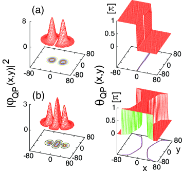
Figure 1: Quasiparticle wave functions [$|\varphi_{\text{QP}}({\bf r})|^{2}$ in units of $10^{-4}/$nm², left, and position-dependent phases $\theta_{\text{QP}}({\bf r})$, right] for the $N=2\rightarrow N=3$ transition in a quantum dot with anisotropy $\eta=0.724$. $\theta_{\text{QP}}({\bf r})$ is 0 or $\pi$, since $\varphi_{\text{QP}}$ can be chosen real for zero magnetic field. The initial state is the ground state ($S=0,S_{z}=0$) for $N=2$ electrons while the final state is (a) the ground state ($S=1/2,S_{z}=1/2$, $E_{1}=20.888$ meV) and (b) the second excited state ($S=1/2,S_{z}=1/2$, $E_{3}=23.013$ meV) for $N=3$ electrons. Lengths in nanometers. $\hbar\omega_{x}=4.23$ meV, $\hbar\omega_{y}=5.84$ meV, $\kappa=12.50$ (GaAs), and $m^{*}=0.067$ (GaAs).

We display in Fig. 1 examples of quasiparticle wave functions (amplitude and phase) for the $N=2\rightarrow N=3$ transition for two different final states (corresponding to the transitions marked 1 and 3 in Fig. 3 below). In Fig. 1(a), $|\varphi_{\text{QP}}|^{2}$ exhibits a two-peak structure separated by one node, while $\Delta\theta_{\text{QP}}=\pi$ (with $x_{L}=-80$ nm and $x_{R}=80$ nm), indicating no phase lapse [see Eq. (5)]. In Fig. 1(b), $|\varphi_{\text{QP}}|^{2}$ exhibits a three-peak structure separated by two nodes, while $\Delta\theta_{\text{QP}}=0$, indicating a PL of $\pi$ [see Eq. (5)]. The nodal structure reflects the good parity of $\varphi_{\text{QP}}$, and it emerges from the many-body EXD calculation (being a priori unknown).

Figure 2: (Color online) The bar-chart for the quasiparticle of the $N=1\rightarrow N=2$ transition in a quantum dot as a function of the strength of the interelectron repulsion (stronger for smaller $\kappa$) and the anisotropy $\eta$. The heights of the bars indicate the weight ${\cal W}$ [Eq. (4)], while shading denotes the quasiparticle transmission phase [$\Delta\theta_{\text{QP}}$ in Eq. (5)]; dark shade (red) denotes $\Delta\theta_{\text{QP}}=\pi$ (no PL) and gray shade (yellow) denotes $\Delta\theta_{\text{QP}}=0$ (occurrence of a PL). The bars are arranged in groups of three around each ($\kappa$,$\eta$) point; the right bar corresponds to the singlet $(s)$ final state, while the middle and left ones correspond to the final triplet states with spin projection $S_{z}=0$ ($t0$) and $S_{z}=1$ ($t1$), respectively. The numbers above the bars denote the energy difference (in meV) between the ground-state singlet and the excited (degenerate) triplets. The effective mass is $m^{*}=0.067m_{e}$ (GaAs). For $\eta=1.0$, $\hbar\omega_{x}=5.0$ meV and $\hbar\omega_{y}=5.0$ meV. For $\eta=0.724$, $\hbar\omega_{x}=4.23$ meV and $\hbar\omega_{y}=5.84$ meV. For $\eta=0.5$, $\hbar\omega_{x}=3.137$ meV and $\hbar\omega_{y}=6.274$ meV. Smaller $\kappa$ and $\eta$ enhance electron localization in the dot. $R_{W}(\kappa=12.50)=1.51$ and $R_{W}(\kappa=1.25)=15.1$.

We discuss next the $N=1\rightarrow N=2$ case. The initial state is the ground state with a single electron (assuming it has a spin up configuration) occupying the lowest single-particle level in $V(x,y)$. The final state, however, is not restricted to the singlet ground state [with ($S=0,S_{z}=0$)] of the $N=2$ quantum dot. Excited states need to be considered, since an excited “doorway” state may be more efficient (have a higher weight) in transmitting the current through the QD. Focussing on the two lowest total energies $E_{k}(S,S_{z})$, we are led to consider three final states, i.e., the ground-state singlet ($S=0,S_{z}=0$), and the two excited triplets ($S=1,S_{z}=0$) and ($S=1,S_{z}=1$), which are degenerate at zero magnetic field. The third triplet state ($S=1,S_{z}=-1$) has zero weight, since flipping of the direction of the initial spin is not allowed. The calculated EXD results are displayed in Fig. 2.

The heights of the bars in Fig. 2 represent the weight ${\cal W}$, while the shading (or color online) of each bar denotes the quasiparticle transmission phase, with a dark shade (online red) denoting $\Delta\theta_{\text{QP}}=\pi$ and a gray shade (online yellow) denoting $\Delta\theta_{\text{QP}}=0$. Results are presented for a weaker $e-e$ repulsion with $\kappa=12.50$ and a much stronger one with $\kappa=1.25$, and for $\eta=1.0$ (circular dot), $\eta=0.724$ (moderate anisotropy), and $\eta=0.5$ (strong anisotropy).

Inspection of Fig. 2 reveals the following systematic trends: (1) The singlet state and the $t0$ triplet have in all instances $\Delta\theta_{\text{QP}}=0$ (with a PL $\theta_{\text{PL}}=-\pi$), while the $t1$ triplet has $\Delta\theta_{\text{QP}}=\pi$ ($\theta_{\text{PL}}=0$, i.e., no PL). (2) The excited $t1$ triplet state has always the largest weight ${\cal W}$, and its relative advantage in ${\cal W}$ compared to the $t0$ and the $s$ states increases both for stronger correlations (smaller $\kappa$) and stronger anisotropies (smaller $\eta$). (3) The singlet-triplet energy gap decreases both for smaller $\kappa$ and $\eta$, i.e., favoring formation of Wigner molecules.

Consequently, the $t1$ triplet state can act as a doorway state for the electron transmission in the case of strong correlations and strong anisotropy. In this case there is no phase lapse ($\theta_{\text{PL}}=0$), as observed experimentally heib05 . Furthermore the experiment excluded the ground-state singlet as being the final state of the two electrons heib05 , in agreement with our analysis here which concluded that the excited $t1$ triplet is a realistic candidate for acting as a doorway state.

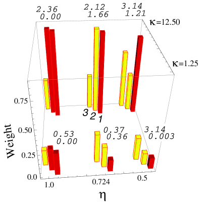
Figure 3: (color online) The bar-chart for the relevant quasiparticles of the $N=2\rightarrow N=3$ transition in a quantum dot as a function of the strength of the interelectron repulsion (through the dielectric constant $\kappa$) and the anisotropy $\eta$. The heights of the bars indicate the weight ${\cal W}$ [Eq. (4)], with a dark shade (red) denoting $\Delta\theta_{\text{QP}}=\pi$ and a gray shade (yellow) denoting $\Delta\theta_{\text{QP}}=0$. In all instances the initial state is the singlet [$(S=0,S_{z}=0)$] ground state of the $N=2$ dot. The bars are arranged in groups of three around each ($\kappa$,$\eta$) point; the rightmost bar corresponds to the final $N=3$ ground state (index 1), while the middle (index 2) and leftmost (index 3) ones correspond to the final $N=3$ two lowest excited states with a non-zero weight. All three final states happen to have a $(S=1/2,S_{z}=1/2)$ magnetic structure. The numbers above the bars denote the energy difference (in meV) between the $N=3$ ground-state and the two lowest excited $(S=1/2,S_{z}=1/2)$ states. The dot parameters are as in Fig. 2.

For the $N=2\rightarrow N=3$ transition, the initial many-body state is assumed to be the ground state of a QD with two electrons, which is always a singlet [$(S=0,S_{z}=0)$]. Again the final state cannot be restricted to the ground state [with ($S=1/2,S_{z}=1/2$)] of the $N=3$ system mikh02li07 , since excited states may act as doorway states. Because the transitions to a final $(S=3/2,S_{z}=3/2)$ or $(S=3/2,S_{z}=1/2)$ state are forbidden (the corresponding ${\cal W}=0$ due to spin blockade), we are led to consider three final states, i.e., the ground-state with $(S=1/2,S_{z}=1/2$) and the two-lowest excited states also with $(S=1/2,S_{z}=1/2)$ mikh02li07 . In Fig. 3, these final states are denoted by the indices 1, 2, and 3, respectively; our results apply unaltered for final states with an $S_{z}=-1/2$ spin projection.

In Fig. 3, we retain the same conventions as in Fig. 2 concerning the height and shadings (colors online) of the bars. Unlike Fig. 2, the final two-lowest excited states in Fig. 3 are not degenerate, and thus in the latter case we list a pair of energy gaps (in meV) with respect to the final ground state. In the circular case ($\eta=1$), there are two degenerate final ground states (with total angular momentum $L=1$ and $L=-1$) mikh02li07 , and the smallest meaningful excitation energy gap needs to be taken between the states with indices 1 and 3 (or 2 and 3).

Inspection of Fig. 3 reveals that a transition to the $N=3$ ground state (marked 1) will always have $\Delta\theta_{\text{QP}}=\pi$ [corresponding to a dark shade (online red)], and thus it will exhibit no lapse in the transmission phase $\theta_{\text{PL}}$ [see Eq. (5)], in contrast to the experimental result. Transmission through a doorway excited state may become possible for smaller $\kappa$ (stronger Coulomb repulsion) and smaller $\eta$ (stronger anisotropy), since as a result (1) the energy gap between the first excited state (index 2) and the ground state diminishes (observe the practically vanishing gap of 0.003 meV for $\eta=0.5$ and $\kappa=1.25$), and (2) the weight ${\cal W}$ of this index-2 final state remains larger than that of the ground state [see the cases with ($\kappa=1.25$, $\eta=0.724$) and ($\kappa=1.25$, $\eta=0.5$)]. Transmission through such an index-2 doorway state will lead to a phase lapse ($\theta_{\text{PL}}=-\pi$), since in this case $\Delta\theta_{\text{QP}}=0$ [gray shade (online yellow)]. A phase lapse in the $N=2\rightarrow N=3$ transition has indeed been observed heib05 . As for the $N=1\rightarrow N=2$ transition, this observation of a phase lapse and our EXD analysis of the $N=2\rightarrow N=3$ transition suggest that the dots in the experiments were strongly deformed and exhibited rather strong ineterelectron correlations.

Conclusions. In summary, focusing on the mesoscopic regime of electron interferometry, and using the Bardeen weak-coupling theory in conjunction with exact diagonalization of the many-body quantum dot Hamiltonian, we have shown for the first two transitions, (a) $N=1\rightarrow N=2$ and (b) $N=2\rightarrow N=3$, nonuniversal behavior of the transmission phases with no phase lapse for (a) and a phase lapse of $\pi$ for (b), in agreement with the experiment heib05 . These results were obtained for a range of dot parameters characterized by shape anisotropy and strong $e-e$ repulsion, with both favoring electron localization and formation of Wigner molecules rop07 ; note2 ; note3 ; note4 . Additionally, our analysis of the quasiparticle wavefunction [Eq. (1)] highlights the dependence of the phase-lapse behavior on the spin configurations of the initial and final states, and the importance of excited doorway states as favored transmission channels. Electron interferometric measurements on dots with characterized shapes note5 , as well as extension of our analysis to a larger number of electrons and the transition to the universal regime, including stronger lead-dot coupling and possibly explicit incorporation of lead states, remain future challenges.

Work supported by the US D.O.E. (Grant No. FG05-86ER45234).

References

- (1) R. Schuster et al., Nature 385, 417 (1997).
- (2) M. Avinun-Kalish et al., Nature 436, 529 (2005).
- (3) See New J. Phys. 9 (2007), Focus articles 111-125.
- (4) C. Karrasch et al., Phys. Rev. Lett. 98, 186802 (2007).
- (5) C. Yannouleas and U. Landman, Rep. Prog. Phys. 70, 2067 (2007), and references therein.
- (6) J. Bardeen, Phys. Rev. Lett. 6, 57 (1961).
- (7) See the introductory part containing Eqs. (1) to (5) in S.A. Gurvitz, Phys. Rev. B 77, 201302 (2008).
- (8) G. Hackenbroich and H.A. Weidenmüller, Phys. Rev. Lett. 76, 110 (1996).
- (9) G. Hackenbroich, Phys. Rep. 343, 464 (2001).
- (10) For calculations of currents with the Bardeen approach, in the context of imaging, see M. Rontani and E. Molinari, Phys. Rev. B 71, 233106 (2005); G. Bester et al., Phys. Rev. B 76, 075338 (2007).
- (11) Y. Li et al., Phys. Rev. B 76, 245310 (2007).
- (12) For the relation between current, density of states, retarded Green’s function, and [Eq. (1)], see J. M. Kinaret et al., Phys. Rev. B 46, 4681 (1992).
- (13) C. Ellenberger et al., Phys. Rev. Lett. 96, 126806 (2006).
- (14) For the EXD spin configurations of an circular QD, see S.A. Mikhailov, Phys. Rev. B 65, 115312 (2002). For an anisotropic QD, see Ref. li07 .
- (15) For see Ref. elle06 , and for see Ref. mikh02li07 .
- (16) Indeed, use of a side plunger, as in Ref. heib05 , is known to lead to shape deformation; see Ref. elle06 , D.M. Zumbühl et al., Phys. Rev. Lett. 93, 256801 (2004), and C. Yannouleas and U. Landman, Proc. Natl. Acad. Sci. (USA) 103, 10600 (2006). Also the estimated meV) / ( meV) =6 for the smaller dots heib05 is higher than that estimated in most other experiments elle06 ; is the charging energy and is the level spacing for two or three electrons heib05 .
- (17) The single-ring ground-state configuration for postulated in Ref. gurv differs from the multi-ring structures for calculated in M. Kong et al., Phys. Rev. E 65 046602 (2002); see also Ref. rop07 .
- (18) For transport measurements and characterization of anisotropic quantum dots, see Ref. elle06 and D.M. Zumbühl et al. in Ref. note3 . In the latter, shallower dots with a small number of electrons, akeen to those in Ref. heib05 , were found to be appropriately characterized by a harmonic confinement.