Coherence and metamagnetism in the two-dimensional Kondo lattice model

Abstract

We report the results of dynamical mean field calculations for the metallic Kondo lattice model subject to an applied magnetic field. High-quality spectral functions reveal that the picture of rigid, hybridized bands, Zeeman-shifted in proportion to the field strength, is qualitatively correct. We find evidence of a zero-temperature magnetization plateau, whose onset coincides with the chemical potential entering the spin up hybridization gap. The plateau appears at the field scale predicted by (static) large-$N$ mean field theory and has a magnetization value consistent with that of $x=1-n_{c}$ spin-polarized heavy holes, where $n_{c}<1$ is the conduction band filling of the noninteracting system. We argue that the emergence of the plateau at low temperature marks the onset of quasiparticle coherence.

I Introduction

The paramagnetic, metallic ground state of heavy fermion compounds Stewart84 ; Lee86 can be interpreted as a Fermi liquid with low coherence temperature and large effective mass. Auerbach86 The origin of the coherence temperature lies in the nature of the quasiparticles, which emerge as a coherent superposition of the Kondo screening clouds of the individual magnetic impurities. Being a Fermi liquid, the heavy fermion ground state is well captured by large-$N$ mean-field theories that predict a renormalized band structure; at this level of approximation, the key properties—such as the effective mass and the Fermi-surface topology—are reproduced.

Mean-field approaches that are static in time, however, do not properly incorporate Kondo screening and hence do not account for the many-body nature of the quasiparticles. Such approaches become questionable when the system is subject to perturbations, such as large temperatures or strong magnetic fields, that have the potential to destroy Kondo screening—hence, the motivation to consider dynamical mean field theories (DMFT), where the Kondo effect is built in.

The problem of a Kondo lattice insulator (symmetric conduction band at half-filling) in a magnetic field has previously been treated approximately using DMFTOhashi05 and exactly using quantum Monte Carlo. Beach04 ; Milat04 In that special case, the only important low-energy scale is the indirect gap separating upper and lower quasiparticle bands. In the metallic case (e.g., filling less than half), there is an additional, smaller energy scale given by the separation between the chemical potential and the top of the lower band. Burdin00 This scale is generically small regardless of the conduction band filling and controls the Fermi liquid properties. As we shall see, it also sets the magnetic field scale for the onset of metamagnetic features.

The static mean field scenario for application of a magnetic field at zero temperature is as follows. As the field strength is increased, the spin up quasiparticle bands descend. The spin up Fermi surface shrinks to a point and disappears as the lower band drops below the chemical potential. Beach05 ; Daou06 ; Kusminskiy07 The resulting half-metallic state Irkhin90 has mean field parameters that are locked at the values obtained before the disappearance of the spin up Fermi surface and are completely insensitive to changes in the field. Beach05 ; Kusminskiy07 As a result, the physical magnetization $-\partial\mathcal{F}/\partial B$ (where $\mathcal{F}$ is the free energy) has a constant slope proportional to the difference between the Landé $g$-factors for the two species. If the $c$- and $f$-electrons couple identically to the applied field, the system is predicted to exhibit a magnetization plateau at a value that depends only on the conduction band filling $n_{c}$. Note that the dimensionless magnetization $M=(n_{c,\uparrow}-n_{c,\downarrow})+(n_{f,\uparrow}-n_{f,\downarrow})$ always shows the plateau behaviour, irrespective of the values of $g_{c}$ and $g_{f}$. This is related to the fact that, in the locked state, the system behaves as a gas of $x=1-n_{c}$ fully spin-polarized, heavy-quasiparticle holes.

Our DMFT results verify this scenario. We find that the magnetization profile begins to develop an inflection at temperatures on the order of the predicted coherence temperature. This feature resembles a plateau smeared by temperature, and we have verified that it sharpens as the temperature is lowered. Moreover, the apparent height of the plateau is consistent with the predicted magnetization value. An analysis of the evolution of the spectral functions with applied field shows that the endpoints of the plateau do coincide with the chemical potential entering and leaving the hybridization gap.

II Model and methods

We consider the Kondo lattice model (KLM) on a square lattice in an external magnetic field $B$:

$$\begin{split}H&=H_{0}+J\sum_{\mathbf{i}}\mathbf{S}^{c}_{\mathbf{i}}\cdot\mathbf{S}^{f}_{\mathbf{i}},\\ H_{0}&=\sum_{\mathbf{k},s}(\epsilon_{\mathbf{k}}-\mu)c^{\dagger}_{\mathbf{k},s}c_{\mathbf{k},s}-g\mu_{B}B\sum_{\mathbf{i}}(S_{\mathbf{i},z}^{c}+S_{\mathbf{i},z}^{f}).\end{split}$$ (1)

Here, $c^{\dagger}_{\mathbf{k},s}$ creates a conduction electron in an extended orbital with wavevector $\mathbf{k}$ and spin projection $s={\uparrow,\downarrow}$ along an axis of quantization chosen parallel to the applied field. The tight-binding dispersion relation is $\epsilon_{\mathbf{k}}=-2t(\cos k_{x}+\cos k_{y})$. At each lattice site $\mathbf{i}$, a local spin-1/2 degree of freedom $\mathbf{S}^{f}_{\mathbf{i}}$ is coupled via $J$ to the $c$-electron spin density $\mathbf{S}^{c}_{\mathbf{i}}=\tfrac{1}{2}\sum_{s,s^{\prime}}c^{\dagger}_{\mathbf{i},s}\bm{\sigma}_{s,s^{\prime}}c_{\mathbf{i},s^{\prime}}$ (represented with the aid of the Pauli spin matrices ${\bm{\sigma}}$). An analogous expression can be written for $\mathbf{S}^{f}_{\mathbf{i}}$ using the localized orbital creation operators $f^{\dagger}_{\mathbf{i},s}$. Since the KLM forbids charge fluctuations on the $f$-orbitals, this representation demands that we impose a strict constraint of one electron per $f$-orbital.

The DMFT approximation neglects spatial fluctuations and thereby omits the $\mathbf{k}$-dependence of the self-energy: i.e., $\bm{\Sigma}_{s}(\mathbf{k},i\omega_{m})\rightarrow\bm{\Sigma}_{s}(i\omega_{m})$. Georges96 ; Maier05 Being local, the self-energy is that of a single impurity in a bath described by the free Hamilton operator $\mathcal{H}_{0}=\sum_{\mathbf{k},s}\tilde{\epsilon}_{\mathbf{k},s}c^{\dagger}_{\mathbf{k},s}c_{\mathbf{k},s}-\tilde{g}_{f}\mu_{B}BS_{i,z}^{f}$. The corresponding local Green bath function is given by

$$\bm{\mathcal{G}}_{s}(i\omega_{m})=\begin{pmatrix}\mathcal{G}^{cc}_{s}(i\omega_{m})&0\\ 0&\mathcal{G}^{ff}_{s}(i\omega_{m})\end{pmatrix}$$ (2)

using $\mathcal{G}^{cc}_{s}(i\omega_{m})=-\int_{0}^{\beta}{\rm d}\tau e^{i\omega_{m}\tau}\langle c^{\phantom{\dagger}}_{\mathbf{0},s}(\tau)c^{\dagger}_{\mathbf{0},s}\rangle_{\mathcal{H}_{0}}$ and the equivalent definition for $\mathcal{G}^{ff}$. The prerequisite for the implementation of DMFT is the ability to solve, for a given bath, the Kondo model,

$$\mathcal{H}=\mathcal{H}_{0}+J\mathbf{S}^{c}_{\mathbf{0}}\cdot\mathbf{S}^{f}_{\mathbf{0}}.$$ (3)

In our calculations, we have opted for the Hirsch-Fye approach. Following Ref. Capponi00, , we expand the Hilbert space to permit charge fluctuations on the $f$-sites and replace the Kondo term by

$$-\frac{J}{4}\biggl{(}\sum_{s}c^{\dagger}_{\mathbf{0},s}f^{\phantom{\dagger}}_{\mathbf{0},s}+\text{h.c.}\biggr{)}^{2}\\ +U\bigl{(}f^{\dagger}_{\mathbf{0},\uparrow}f^{\phantom{\dagger}}_{\mathbf{0},\uparrow}-1/2\bigr{)}\bigl{(}f^{\dagger}_{\mathbf{0},\downarrow}f^{\phantom{\dagger}}_{\mathbf{0},\downarrow}-1/2\bigr{)}.$$ (4)

At the expense of two discrete Hubbard-Stratonovich fields, we can decompose the (perfect square) hybridization and Hubbard terms, and readily implement the above interaction within the framework of the Hirsch-Fye algorithm. Capponi00 In the limit $U\rightarrow\infty$, charge fluctuations on the $f$-orbitals are suppressed and the squared hybridization reduces to the desired Kondo term. The efficiency of this approach lies in the fact that $U(f^{\dagger}_{\mathbf{0},\uparrow}f_{\mathbf{0},\uparrow}-1/2)(f^{\dagger}_{\mathbf{0},\downarrow}f_{\mathbf{0},\downarrow}-1/2)$ is a conserved quantity Capponi00 for the considered class of $\mathcal{H}_{0}$, which does not include hybridization terms between the bath and impurity orbital. Typically, $\beta U\simeq 30$ suffices to ensure that double occupancy drops down to $\langle f^{\dagger}_{\mathbf{0},\uparrow}f_{\mathbf{0},\uparrow}f^{\dagger}_{\mathbf{0},\downarrow}f_{\mathbf{0},\downarrow}\rangle=0.0005\pm 0.0005$ and that $\langle\sum_{s}f^{\dagger}_{\mathbf{0},s}f_{\mathbf{0},s}\rangle=1$ to the same precision. Since charge fluctuations on the $f$-sites are suppressed by the Hubbard interaction, the local Green function, as obtained from the Hirsch-Fye alogorithm, is diagonal in the large-$U$ limit and is given by

$$\mathbf{G}_{s}(i\omega_{m})=\frac{1}{\bm{\mathcal{G}}_{s}^{-1}(i\omega_{m})-\bm{\Sigma}_{s}(i\omega_{m})}.$$ (5)

Self-consistency requires that the local Green function, as determined from the effective impurity problem, matches that of the lattice:

$$\mathbf{G}_{s}(i\omega_{m}) \equiv \frac{1}{N}\sum_{\mathbf{k}}\frac{1}{\mathbf{G}_{0,s}^{-1}(\mathbf{k},i\omega_{m})-\bm{\Sigma}_{s}(i\omega_{m})}$$ (6)

$$= \frac{1}{\bm{\mathcal{G}}_{s}(i\omega_{m})-\bm{\Sigma}_{s}(i\omega_{m})}.$$

Here, $\mathbf{G}_{0,s}(\mathbf{k},i\omega_{m})$ is the free lattice Green function [corresponding to $H_{0}$ in Eq. (1)]. 

Hence, for a given bath Green function $\bm{\mathcal{G}}_{s}(i\omega_{m})$, we extract the self-energy from the impurity solver and, exploiting Eq. (6), recompute the bath Green function with

$$\bm{\mathcal{G}}_{s}^{-1}(i\omega_{m})=\bm{\Sigma}_{s}(i\omega_{m})\\ +\biggl{(}\frac{1}{N}\sum_{\mathbf{k}}\frac{1}{\mathbf{G}_{0,s}^{-1}(\mathbf{k},i\omega_{m})-\bm{\Sigma}_{s}(i\omega_{m})}\biggr{)}^{-1}.$$ (7)

The procedure is repeated until convergence is achieved. As noted above, in the limit $U\rightarrow\infty$ the local Green function, self-energy, and bath Green function are all diagonal. Accordingly, the self-consistency [see Eq. (6)] is equivalent to two scalar equations:

$$\frac{1}{N}\sum_{k}\frac{{\mathcal{G}_{0,s}^{cc}}^{-1}(i\omega_{m})-\Sigma^{cc}_{s}(i\omega_{m})}{{G_{0,s}^{cc}}^{-1}(\mathbf{k},i\omega_{m})-\Sigma_{s}^{cc}(i\omega_{m})}=1,$$ (8)

$$G_{0,s}^{ff}(i\omega_{m})=\mathcal{G}^{ff}_{0,s}(i\omega_{m}).$$ (9)

The last equality follows from the fact that $G_{0,s}^{ff}(\mathbf{k},i\omega_{m})$ has no $\mathbf{k}$ dependence.

Having determined the self-energy, one can readily compute the single particle Green function $G^{cc}_{s}(\mathbf{k},i\omega_{m})$ and extract the spectral function $A(\mathbf{k},\omega)$ with a stochastic analytical continuation method. Sandvik98 ; Beach04a

Figure 1: The upper and lower hybridized bands $E_{\mathbf{k}}^{\pm}$ are plotted over a trajectory bounding one octant of the Brillouin zone. The grey line-width is proportional to the $c$-electron spectral weight. The indirect gap $2\Delta$ and the optical gap $2V$ are indicated. The corresponding $c$-electron density of states $\rho_{c}(\omega)$ is plotted to the right on the same energy scale. In magnification, the region around the gap is illustrated with the filled Fermi sea shaded in grey, revealing a small amount of headroom $\varepsilon_{t}\ll 2\Delta$ in the lower band. In the lower two panels, the small, noninteracting Fermi surface is contrasted with the large interacting one.

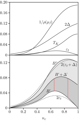
Figure 2: (Upper panel) As a function of the bare filling $n_{c}$, the inverse quasiparticle DOS $1/\rho(\mu_{f})$ and the indirect gap $2\Delta$ are compared to the energy scales defined by the Kondo temperature $T_{\text{K}}$ (with $k_{B}=1$) and the width $\varepsilon_{t}$ of unfilled states at the top of the lower band. (Lower panel) The dashed lines at $2\epsilon_{t}$ and $2(\epsilon_{t}+\Delta)$ mark the plateau endpoints that arise from a purely rigid shifting of the bands (in units where $\mu_{B}g=1$). The shaded areas between $B^{\prime}$ and $B^{\prime\prime}$ indicate the extent of the locked region as calculated using the fully self-consistent mean field equations. The discrepancy is a result of higher order changes in the mean field parameters. We expect that the inclusion of $V$ phase fluctuations restricts plateau formation to between $B^{\prime}$ and $B^{\prime}+\Delta^{\prime}$ (roughly) and leads to a slow disintegration of the heavy fermion state between $B^{\prime}+\Delta^{\prime}$ and $B^{\prime\prime}$. The vertical dashed (red) lines between $B^{\prime}$ and $B^{\prime}+\Delta^{\prime}$ at $n_{c}=0.65$ and $n_{c}=0.85$ appear again as horizontal dashed (red) lines in Fig. 6.

Figure 3: The magnetization of conduction $m_{c}$ and local moments $m_{f}$, computed via DMFT, are plotted as a function of magnetic field at various temperatures. In the upper panel, the lines running through the $f$-electron data points are fit to the forms $\tanh(S^{\text{eff}}g\mu_{B}B\beta)$. At $\beta t=5$, $2S^{\text{eff}}=1.03$ and at $\beta t=10$, $2S^{\text{eff}}=0.65$. In the lower panel, the magnetization profile is marked with three regions. A sketch of the spin resolved density of states as deduced from the single particle spectral function (See Fig. 5) is given in each region.

III Mean field picture

Free electrons moving via nearest-neighbour hopping on the square lattice have a density of states (DOS)

$$\rho_{0}(\omega)=\frac{1}{2\pi^{2}t}\mathcal{K}\Bigl{(}\!\sqrt{1-(\omega/4t)^{2}}\,\Bigr{)}\theta(16t^{2}-\omega^{2}),$$ (10)

written in closed form in terms of an elliptic integral of the first kind, $\mathcal{K}(x)$. The function has support in the region $-4t<\omega<4t$ and thus a bandwidth $W=8t$. It is smooth and continous, except at the step-like band edges and at $\omega=0$ (a van Hove singularity), where it diverges as $\rho_{0}(\omega)\sim\frac{1}{2\pi^{2}t}\log\frac{16t}{|\omega|}$. [Numerical evaluation of Eq. (10) can be carried out very efficiently using series expansion; see Appendix A.]

At the mean-field level, the interacting Kondo lattice system is modelled by a bilinear effective Hamiltonian that includes both $c$- and $f$-electrons. This can be obtained from the saddle-point of the Hubbard-Stratonovich decomposition of Eq. (4):

$$\begin{pmatrix}c^{\dagger}_{\mathbf{k}}&f^{\dagger}_{\mathbf{k}}\end{pmatrix}\!\begin{pmatrix}\epsilon_{\mathbf{k}}\!-\!\mu_{c}\!-\!\tfrac{1}{2}g\mu_{B}B\sigma_{z}&-V\\ -V&-\mu_{f}\!-\!\tfrac{1}{2}g\mu_{B}B\sigma_{z}\end{pmatrix}\!\begin{pmatrix}c_{\mathbf{k}}\\ f_{\mathbf{k}}\end{pmatrix}\!.$$ (11)

In the usual way, hybridization between the $c$-electrons and the dispersionless band of $f$-electrons leads to a renormalized, quasiparticle dispersion

$$E^{\pm}_{\mathbf{k},s}=\frac{1}{2}\biggl{[}\epsilon_{\mathbf{k}}-sg\mu_{B}B\pm\sqrt{(\epsilon_{\mathbf{k}}-b)^{2}+4V^{2}}\biggr{]}$$ (12)

and a quasiparticle DOS $\rho(\omega)=\rho_{c}(\omega)+\rho_{f}(\omega)$, where

$$\rho_{c}(\omega)=\rho_{0}(\omega-V^{2}/\omega+b)$$ (13)

and $\rho_{f}(\omega)=(V^{2}/\omega^{2})\rho_{c}(\omega)$. Here $b=\mu_{c}-\mu_{f}$ is the chemical energy to transmute the $c$- and $f$-electron character of a particle, and $V$ is a hybridization energy determined self-consistently via $V\sim J\sum_{s}\langle c^{\dagger}_{\mathbf{k},s}f_{\mathbf{k},s}\rangle$. The spectral weight vanishes outside the lower $[\omega_{1},\omega_{2}]$ and upper $[\omega_{3},\omega_{4}]$ hybridized bands, where $\omega_{i}$ ($i=1,2,3,4$) denote the four ordered roots of $\pm 4t=\omega-V^{2}/\omega+b$.

The mean field equations can be written compactly as

$$\sum_{s}\int_{I}\!d\omega\,\rho_{c}(\omega)f(\omega-\mu_{f,s})\begin{Bmatrix}1\\ V^{2}/\omega^{2}\\ -\mathcal{J}/2\omega\end{Bmatrix}=\begin{Bmatrix}n_{c}\\ 1\\ 1\end{Bmatrix},$$ (14)

where the integral is taken over the disjoint interval $I=[\omega_{1},\omega_{2}]\cup[\omega_{3},\omega_{4}]$, and $\mu_{f,s}$ is shorthand for $\mu_{f}\pm g\mu_{B}B/2$. The first two equations fix the $c$- and $f$-electron occupation (to $n_{c}$ and 1, respectively), and the third enforces the self-consistency condition on $V$. We have written $\mathcal{J}=(\text{const.})\times J$ to allow for the fact that different mean field decompositions lead to a different numerical prefactor. In each spin channel, $2\Delta=\omega_{3}-\omega_{2}$ is the smallest indirect gap, and $2V$ is the threshold for optical excitations. Dordevic01 ; Millis87 Figure 1 illustrates the zero-temperature, zero-magnetic-field solution appropriate for band filling $0<n_{c}<1$. An additional energy scale $\varepsilon_{t}=\omega_{2}-\mu_{f}$, representing the headroom at the top of the lower band, is indicated.

An artifact of the mean field treatment is that the hybridization matrix element has an anomolous expectation value that vanishes with heating at a second-order phase transition. (The true Kondo physics is that of a crossover.) There is a critical temperature $T_{\text{c}}$ such that as $T\to T_{\text{c}}$ from below, $V,\mu_{f}\to 0$ and $b\to\mu_{c}$. As the quasiparticles disintegrate into their separate $c$- and $f$-character consituents, the corresponding densities of states return to their free values: $\rho_{c}(\omega)\to\rho_{0}(\omega+\mu_{c})$ and $\rho_{f}(\omega)\to\delta(\omega)$. In this limit, Eq. (14) reduces to

$$\frac{2}{\mathcal{J}}=\int_{-4t}^{4t}\!d\omega\,\biggl{[}\rho_{0}(\omega)\frac{\tanh[(\omega-\mu_{c})/2T_{\text{c}}]}{\omega-\mu_{c}}\\ -\frac{\rho_{0}(\omega)-\rho_{0}(\mu_{c})}{\omega-\mu_{c}}\biggr{]}-\rho_{0}(\mu_{c})\log\frac{4t-\mu_{c}}{4t+\mu_{c}},$$ (15)

where $\mu_{c}(n_{c})$ takes its noninteracting value, determined implicitly by

$$2\int_{-4t}^{4t}\rho_{0}(\omega)f(\omega-\mu_{c})=n_{c}.$$ (16)

The critical temperature scales as $T_{\text{c}}\sim\alpha W$, where the constant of proportionality is a function of the band filling alone. (For a flat DOS, $T_{\text{c}}=0.567n_{c}\times\alpha W$.) The small parameter $\alpha=e^{-1/\mathcal{J}\rho_{0}(\mu_{c})}$ renormalizes the bandwidth down to the Kondo scale; hence it is natural to identify a Kondo temperature $T_{\text{K}}\equiv T_{\text{c}}$. On the square lattice, the value of $T_{\text{K}}$ is always nonzero for $n_{c}>0$. $T_{\text{K}}$ is compared to the important zero-temperature energy scales in the upper panel of Fig. 2. A value $\mathcal{J}/t=1.631$ was chosen so that $\partial M/\partial B\bigr{\rvert}_{B=0}=\rho(\mu_{f})$ matches the DMFT results for $J/t=1.6$ and $n_{c}=0.85$. (We set $g\mu_{B}=1$ for the remainder of this section.)

At zero temperature, where the hybridization is at its strongest, the Fermi function in Eq. (14) cuts off the integration at $\mu_{f,s}$. There are three possibilities: (I) $\omega_{1}<\mu_{f,s}<\omega_{2}$; (II) $\omega_{1}<\mu_{f,\downarrow}<\omega_{2}$ and $\omega_{2}<\mu_{f,\uparrow}<\omega_{3}$; (III) $\omega_{1}<\mu_{f,\downarrow}<\omega_{2}$ and $\omega_{3}<\mu_{f,\uparrow}<\omega_{4}$. In cases I and III, both spin up and spin down quasiparticles have a Fermi surface. In case II, the chemical potential lies in the spin up hybridization gap. As a consequence, the upper limit of integration in the spin up channel is $\omega_{2}$, and $\mu_{f,\uparrow}$ no longer enters the equations. The magnetic field enters only indirectly through $\mu_{f,\downarrow}$, and thus the system becomes insensitive to changes in magnetic field. In particular, this leads to a plateau in the magnetization. Note that $\mu_{f,\downarrow}=\text{const.}$ and hence $\mu_{f,\uparrow}=\text{const.}+B$, which means that the upper band descends at twice the rate it does in case I, where $\mu_{f,\uparrow}\sim\mu_{f}\rvert_{B=0}+B/2$. The plateau terminates when $\mu_{f,\uparrow}$ reaches the lower edge of the upper hydridized band.

The leading edge of the plateau can be determined by solving for the field $B^{\prime}$ at which $\mu_{f,\uparrow}=\omega_{2}$ and $\mu_{f,\downarrow}=\omega_{2}-B^{\prime}$. Since the mean field parameters are locked beyond $B^{\prime}$, the far edge is simply $B^{\prime\prime}=B^{\prime}+2\Delta^{\prime}$, where $2\Delta^{\prime}$ is the size of the indirect hybridization gap at $B=B^{\prime}$ (and its size throughout $B^{\prime}<B<B^{\prime\prime}$). This argument for the location of the far edge is flawed in one respect: when $B>B^{\prime\prime}$, the system is expected to enter region III, but the mean field equations in that region turn out to be pathological ($V$ begins to increase rapidly with $B$). Indeed, energetic considerations tell us that for $B=B^{\prime\prime}[1-O(\alpha^{2})]$ the $V=0$ normal state becomes energetically favourable. Beach05 Nonetheless, this apparent first-order collapse to the normal state cannot survive the inclusion of phase fluctuations in $V$, which smooths out the destruction of the heavy fermion state over a width $\Delta$. Hence, we expect to find a plateau in $B^{\prime}<B<B^{\prime}+\Delta^{\prime}$ and a crossover to the normal state in $B^{\prime}+\Delta^{\prime}<B<B^{\prime\prime}=B^{\prime}+2\Delta^{\prime}$. The predicted extent of the plateau is shown in the lower panel of Fig. 2.

The mean field picture describes $x=1-n_{c}$ heavy holes, which spin-align with the applied field and become completely polarized at $B^{\prime}$. Along the plateau, the value of the magnetization is $M=(n_{c\uparrow}+n_{f\uparrow})-(n_{c\uparrow}+n_{f\uparrow})=x[1-O(\alpha^{2})]$. This follows because $n_{c\uparrow}\simeq n_{f\uparrow}\simeq 1$ and $n_{c\downarrow}\simeq n_{f\downarrow}\simeq 1-x/2$ when the chemical potential sits in the spin up hybridization gap. In the Kondo limit ($\mathcal{J}\ll W$), $\alpha$ is exponentially small and corrections of order $\alpha^{2}$ are completely negligible. Hence, the plateau has a height of almost exactly $M=x$.

IV DMFT results

The mean-field picture of the metamagnetic transition and the associated change in the Fermi surface topology is a direct consequence of coherence. To confirm this, we have carried out temperature and magnetic field DMFT scans at $J/t=1.6$ and electron density $n_{c}=0.85$ (see Fig. 3). This choice of parameters sets the single impurity Kondo scale to $T_{K}/t\simeq 0.09$. At temperature scales larger than the Kondo scale, one expects the local moments to be essentially free with magnetization

$$m_{f}\equiv 2\langle S^{f}_{\mathbf{i},z}\rangle=\tanh\bigl{(}S^{\text{eff}}\beta g\mu_{B}B\bigr{)},$$ (17)

where $S^{\text{eff}}$ allows for a renormalization of the impurity moment. At $\beta t=5$, the DMFT data (see top panel of Fig. 3) for $m_{f}$ follows this form with $S^{\text{eff}}\simeq 1/2$ to considerable accuracy, thereby showing that the system is in the high temperature local moment regime. The polarization of the conduction electrons is opposed to the applied magnetic field because the antiferromagnetic Kondo interaction generates a negative effective magnetic field. Beach04 ; Kusminskiy07 In the vicinity of the Kondo temperature, at $\beta t=10$, the magnetization curve $m_{f}$ can roughly be accounted for with the free moment form of Eq. (17), albeit with $S^{\text{eff}}\simeq 1/3$. This reduction is consistent with the onset of Kondo screening. At temperatures $\beta t>30$, which we argue are well below the coherence temperature, three distinct regions denoted by I, II, and III are apparent in the data, as shown in Fig. 3. Our understanding of those features relies on the single particle spectral function below the coherence temperature and the associated change in the Fermi surface topology as a function of the magnetic field.

Figure 4: The $c$-electron spectral function $A(\mathbf{k},\omega)$ in zero field is plotted for three progressively lower temperatures. The legend at the top indicates the false color values.

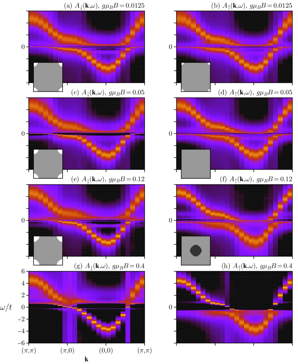
Figure 5: Low temperature, $\beta t=40$, spectral function in the up (left) and down (right) spin sector as a function of magnetic field. We use the same scale as in Fig. 4.

In zero magnetic field and at our lowest temperature, $\beta t=40$ [see Fig. 4(c)], the single particle spectral function follows the hybridized band picture of the mean-field calculation (cf. Fig. 1), reflecting the coherent heavy fermion metallic state with Luttinger volume including both conduction and localized electrons and large effective mass. Introducing a magnetic field leads to competing effects. One possibile outcome is that Kondo screening is completely suppressed—thus triggering the breakdown of the heavy-quasiparticle, the heavy fermion coherent state, and the associated large Fermi surface. Another is that partial Kondo screening persists and that the heavy fermion metallic state survives in some form. Fig. 5 supports the latter. In particular, in region I [Fig. 5(a),(b)] the two-fold spin degeneracy of the spectral function is lifted and the spin down (up) band shifts to higher (lower) energies, thereby producing hole-like Fermi surfaces of different size centered around $\mathbf{k}=(\pi,\pi)$. [The fact that the spin down (up) band shifts up (down) in energy and yet $m_{c}<0$ is a consequence of some subtle rearrangement of spectral weight.] The onset of region II [Fig. 5(c),(d)] is marked by the vanishing of the spin up Fermi surface: the chemical potential lies within the hybridization gap, and the lower spin up band is completely filled. This sudden change in the Fermi surface topology is the origin of the cusp-like feature separating regions I and II. Note that the magnetization data of Fig. 3 supports the sharpening of the cusp as the temperature is lowered. Region III [Fig. 5(e),(f)] is again characterized by a change in the topology of the Fermi surface. Here the spin up valence band drops below the chemical potential, thereby forming an electron-like spin down Fermi surface centred around the $\mathbf{k}=(0,0)$ point. Across regions I, II, and III, the spin down Fermi surface evolves continuously with a growing hole-like Fermi surface centered around $\mathbf{k}=(\pi,\pi)$. A sketch of the spin-resolved density of states in the three regions is given in Fig. 3. At very high magnetic fields [Fig. 5(g),(h)] the spectral function progressively tends towards that of a Zeeman split cosine band.

The onset of the plateau-like feature in the magnetization curve as a function of temperature can be used as measure of the coherence temperature. At $J/t=1.6$ and $n_{c}=0.85$, Fig. 3 provides a rough estimate of this scale: $T_{\text{coh}}/t\simeq 1/30$. Given $T_{\text{coh}}$, it is interesting to analyze the temperature dependence of the single particle spectral function (see Fig. 4). Already at temperatures $T/t=1/5$ and $T/t=1/10$ above $T_{K}/t\simeq 0.09$, features of the hybridized bands are apparent. At those temperatures the magnetization curve is featureless since the coherence or hybridization gap is not formed. At $T/t=1/40<T_{\text{coh}}$ (Fig. 4c) the coherence gap is well formed and the plateau feature in the magnetization curve is apparent.

Figure 6: Total magnetization, $M=m_{c}+m_{f}$, as function of temperature and band filling. The plateaux at $x=1-n_{c}$, predicted by the mean field theory, are indicated with horizontal dashed (red) lines and correspond to the vertical dashed (red) lines in the lower panel of Fig. 2.

As argued in Sec III, the height of the magnetization plateau, $M=1-n_{c}$, follows from the Luttinger sum rule. Fig. 6 plots the total magnetization $M=m_{c}+m_{f}$ at two different conduction band fillings, $n_{c}=0.85$ and $n_{c}=0.65$. As the temperature decreases, a plateau-like feature precisely at $1-n_{c}$ emerges. For comparison, we have plotted the mean-field prediction as obtained from Fig. 2. Note that the initial slope in the magnetization curve is related to the effective mass, which is inversely proportional to the coherence temperature. Hence, at low band fillings, lower temperature values are required to reveal the plateau feature.

V Conclusions

The interaction of conducting electrons with local impurities often gives rise to complicated nonlinearities in magnetic response (often described as metamagnetism). Below the coherence temperature, we find that the magnetization profile of the Kondo lattice system shows a plateau, whose onset is linked to the vanishing of the Fermi surface in one spin sector. The relevant energy scale corresponds to the headroom above the chemical potential in the lower hybridized band. As a consequence of the Luttinger sum rule, the total magnetization is locked to the value $M=1-n_{c}$ throughout the plateau. The plateau survives up to magnetic fields at which the quasiparticles begin to break apart. At high fields, the system is once again characterized by Fermi surfaces in both spin sectors, which smoothly evolve with increasing field back to those expected for the Zeeman-split bare conduction band.

We have reached these conclusions on the basis of dynamical and static mean field calculations, both of which are consistent with the scenario we have outlined. There is one important disagreement between the two theories. At large fields, the DMFT shows that once the chemical has traversed the gap, it enters the upper hybridized band, and the system again becomes a heavy metal with two Fermi surfaces. The behavior of the static mean field equations after the reentry into the upper band is pathological. Energy considerations suggest a first-order collapse back to the normal state. There is no evidence of this within DMFT, and we expect that phase fluctuations of the hybridization field are responsible for washing out this false transition.

In closing, this work establishes that the metamagnetic behavior of Kondo systems is intimately related to coherence. We have shown that the magnetization profile of a Kondo system is a useful probe of the onset of coherence at low temperatures. The location of the incipient plateau reveals the important energy scales; its height is a direct measure of the Luttinger sum rule.

Appendix A Bare Density of States

Numerical evaluation of the bare DOS is readily accomplished using a power series expansion about the Van Hove singularity at $\omega=0$:

$$\rho_{0}(\omega)=\frac{1}{2\pi^{2}t}\biggl{[}\log\frac{16t}{|\omega|}+\biggl{(}\log\frac{16t}{|\omega|}-1\biggr{)}\biggl{(}\frac{\omega}{8t}\biggr{)}^{2}+\frac{9}{4}\biggl{(}\log\frac{16t}{|\omega|}-\frac{7}{6}\biggr{)}\biggl{(}\frac{\omega}{8t}\biggr{)}^{4}+\frac{25}{4}\biggl{(}\log\frac{16t}{|\omega|}-\frac{37}{30}\biggr{)}\biggl{(}\frac{\omega}{8t}\biggr{)}^{6}+\cdots\biggr{]}$$ (18)

Truncating the expansion at eighth order in $\omega/t$ results in a relative error of at most $10^{-7}$ in the region $-t<\omega<t$ and $10^{-2}$ in the region $-4t<\omega<4t$.

References

- (1) G. R. Stewart, Rev. Mod. Phys. 56, 755 (1984).
- (2) P. A. Lee, T. M. Rice, J. W. Serene, L. J. Sham, and J. W. Wilkins, Comm. in Condensed Matter Phys. 12, 99 (1986).
- (3) A. Auerbach and K. Levin, Phys. Rev. Lett. 57, 877 (1986).
- (4) T. Ohashi, S. Suga, and N. Kawakami, J. Phys. Condens. Matter 17, 4547 (2005); T. Ohashi, A. Koga, S. Suga, N. Kawakami, Physica B 359–361, 738 (2005); ibid., Phys- Rev. B 70, 245104 (2004).
- (5) K. S. D. Beach, P. A. Lee, and P. Monthoux, Phys. Rev. Lett. 92, 26401 (2004).
- (6) I. Milat, F. F. Assaad, and M. Sigrist, Eur. Phys. J. B 38, 571 (2004).
- (7) S. Burdin, A. Georges, and D. R. Grempel, Phys. Rev. Lett. 85, 1048 (2000).
- (8) R. Daou, C. Bergemann, and S. R. Julian, Phys. Rev. Lett. 96, 026401 (2006).
- (9) K. S. D. Beach, arXiv:cond-mat/0509778v2.
- (10) S. Viola Kusminskiy, K. S. D. Beach, A. H. Castro Neto, David K. Campbell, arXiv:0711.2074v1.
- (11) V. Yu. Irkhin and M. I. Katsnelson, J. Phys.: Condens. Matter 2, 8715 (1990).
- (12) A. Georges, G. Kotliar, W. Krauth, and M. J. Rozenberg, Rev. Mod. Phys. 68, 13 (1996).
- (13) T. Maier, M. Jarrell, T. Prushke, and M. H. Hettler, Rev. Mod. Phys. 77, 1027 (2005).
- (14) S. Capponi and F. F. Assaad, Phys. Rev. B 63, 155114 (2001).
- (15) A. Sandvik, Phys. Rev. B 57, 10287 (1998).
- (16) K. S. D. Beach, arXiv:cond-mat/0403055.
- (17) K. Pesz and R. W. Munn, J. Phys. C: Solid State Phys. 19, 2499 (1986).
- (18) T. M. Hong and G. A. Gehring, Phys. Rev. B 46, 231 (1992).
- (19) F. F. Assaad, Phys. Rev. B 70, 020402(R) (2004).
- (20) S. V. Dordevic, D. N. Basov, N. R. Dilley, E. D. Bauer, and M. B. Maple, Phys. Rev. Lett. 86, 684 (2001).
- (21) A. J. Millis and P. A. Lee, Phys. Rev. B 35, 3394 (1987); A. J. Millis, M. Lavagna, and P. A. Lee, Phys. Rev. B 36, 864 (1987).